Dynamical Evolution and Galaxy Populations
in the Cluster ABCG 209 at z=0.2  
 
 

da “Aprire su Paidea”, a cura di Edda Ducci

Dedico un ringraziamento speciale a tutti coloro che hanno saputo parlare da anima ad anima, aiutandomi a portare in superficie la bellezza dell’interiore. Le loro parole, ma soprattutto i loro silenzi carichi di significato mi hanno permesso di superare tutte le difficoltà con la forza del sentire.

Grazie ai miei educatori che hanno saputo distinguere tra sapere e sapere impedendomi di diventare una semplice vite della gabbia della mera comunità accademica che offende e lede la felice agilità retaggio della libertà del singolo.

Introduction

Understanding the formation and the evolution of galaxies and galaxy clusters, has always been of great interest for astronomers.

Although the study of galaxy clusters has a long history, there are many unresolved and still debated questions.

-

When did galaxies and galaxy clusters form? And in which order?

-

How do the global properties of clusters evolve?

-

Which are the steps in cluster evolution that cause the luminosity and morphological segregation of galaxies?

-

How do the gas and the galaxy stellar populations evolve in clusters?

The main current challenges in understanding the properties of galaxy clusters is the evidence that many of them are still in an early stage of formation. Cluster of galaxies are no longer believed to be simple, relaxed structures, but are interpreted within the hierarchical growth via mergers of smaller groups/clusters. Although many observational evidences exist that there is a large fraction of clusters which are really still forming, the fundamental question raised from these observations remain: are clusters generally young or old?

To address this issue one needs to have measurements of subclustering properties of a large sample of clusters, but at the same time it is fundamental to precisely characterize galaxies belonging to different structures and environments inside a single cluster.

Due to the complexity in the distribution of different cluster constituents (galaxies, gas, dark matter), combined multi-wavelength observations and detailed analysis are necessary to understand the complex history of clusters formation and evolution.

Up to now complete and detailed analysis have been performed on many nearby clusters. Moreover, the use of large ground-based telescopes (4-8m diameter) and of the Space Telescope allowed studies on clusters at high redshifts: up to z $\sim$ 1. This increasing amount of data induced astronomers to perform statistical studies, which are crucial to trace the large scale structure and to provide a measure of the mean density of the universe.

Clusters at intermediate–redshifts (z = 0.1-0.3) seem to represent an optimal compromise for these studies, because they allow to achieve the accuracy needed to study the connection between the cluster dynamics and the properties of galaxy populations and, at the same time, to span look–back time of some Gyr.

This thesis work is focused on the analysis of the galaxy cluster ABCG 209, at z$\sim$ 0.2, which is characterized by a strong dynamical evolution. The data sample used here consists in new optical data (EMMI-NTT B, V and R band images and MOS spectra) and archive data (CFHT12k B and R images), plus archive X-ray (Chandra) and radio (VLA) observations.

After a short historical overview and a brief description of cluster properties (Chapter 1), the optical analysis of the cluster is carried out by studying the internal structure and the dynamics of the cluster, through the spectroscopic investigation of member galaxies (Chapter 2). The luminosity function, which is crucial in order to trace the photometric properties of the cluster, such as luminosity segregation, and for understanding the evolving state of this cluster is studied in Chapter 3. The investigation of the connection between the internal cluster dynamics and the star formation history of member galaxies was performed through two independent approaches : i) the study of the colour–magnitude relation and of the luminosity function in different environments (Chapter 4) and ii) the spectral classification of cluster galaxies, and the comparison with stellar evolution models (Chapter 5).

Chapter 1 Cluster properties

Galaxy clusters are the largest gravitationally bound structures in the universe, which have collapsed very recently or are still collapsing. They typically contain 10²-10³ galaxies in a region of few Mpc, with a total mass that can be larger than 10¹⁵ solar masses. X-ray observations show that clusters are embedded in an “intra–cluster medium” of hot plasma, with typical temperatures ranging from 2 to 14 keV, and with central densities of $\sim$ 10^-3 atoms cm^-3. The hot plasma is detected through X-ray emission, produced by thermal bremsstrahlung radiation, with typical luminosity of L_X $\sim$ 10^43-45 erg s^-1. Radio observations prove the existence of radio emission associated with galaxy clusters. This is synchrotron emission due to the interaction between non–thermal population of relativistic electrons (with a power-law energy distribution) and a magnetic field.

Clusters are interesting objects both as individual units and as tracers of large scale structures. They offer an optimal laboratory to study many different astrophysical problems such as the form of the initial fluctuation spectrum, the evolution and the formation of galaxies, the environmental effects on galaxies, and the nature and quantity of dark matter in the universe.

An increasing amount of data revealed that clusters are very complex systems and pointed out the necessity of studying these structures using various complementary approaches.

In this chapter, I will give first a short historical overview of the study of galaxy clusters, and then I will outline their basic properties at different wavelengths.

1.1 Historical Overview

The study of galaxy clusters has a long history: early observations of “nebulae” , described at the beginning of the XX century (Wolf 1902, 1906) already recognized the clustering of galaxies. Later, the work of Shapley and Ames (1932) drew out, for the first time, many of the features of the large scale galactic distribution. From their studies of the distribution of galaxies brighter than 13^th magnitude, they were able to delineate the Virgo cluster, several concentrations of clusters at greater distances, and to point out the asymmetry in the distribution of galaxies between the northern and the southern galactic hemispheres.

In 1933 Fritz Zwicky (1933) first noticed that the dynamical determinations of cluster masses require a very large amount of unseen material (dark matter). Since then, galaxy clusters have been studied in detail and at different wavelengths, but his original conclusion remained unchanged. Few years later, he discussed the clustering of nebulae from a visual inspection of photographic plates of the survey from the 18 inch (0.5 m) Schmidt telescope at Palomar, by noting that elliptical galaxies are much more strongly clustered than late-type galaxies (Zwicky 1938, Zwicky 1942).

The first systematic optical study of clusters properties is due to Abell (1958), who compiled an extensive, statistically complete, catalogue of rich clusters. He defined as cluster the region of the sky where the surface numerical density of galaxies is higher than that of the adjacent field, and obtained an estimate of the redshift from the magnitude of the tenth brightest galaxy in the cluster. In the compilation of the catalogue, he selected galaxy clusters on the basis of the following criteria: i) the cluster had to contain at least 50 galaxies in the magnitude range m₃–m₃+2, where m₃ is the magnitude of the third brightest galaxy; ii) these galaxies had to be contained within a circle of radius R_A= 1.5 h${}_{100}^{-1}$ Mpc (Abell radius); iii) the estimated cluster redshift had to be in the range 0.02 $\leq$ z $\leq$ 0.20. Abell gave also an estimate of position of the centre and of the distance of clusters. The resulting catalogue, consisting of 1682 clusters, remained the fundamental reference for studies on galaxy clusters until Abell, Corwin, & Olowin (1989) published an improved and expanded catalogue, including the southern sky. These catalogues constituted the basis for many cosmological studies and still now represent important resources in the study of galaxy clusters.

Zwicky and his collaborators (Zwicky et al. 1961-1968) constructed another extensive catalogue of rich galaxy clusters , by identifying clusters as enhancements in the surface number density of galaxies on the National Geographic Society-Palomar Observatory Sky Survey (Minkowsky & Abell, 1963), but using selection criteria less strict than Abell’s catalogue.

He determined the boundary (scale size) of clusters by the contour (or “isopleth”) where the surface density of galaxies falls to twice the local background density. This isopleth had to contain at least 50 galaxies in the magnitude range m₁–m₁+3, where m₁ is the magnitude of the brightest galaxy. No distance limits were specified, although very nearby clusters, such as Virgo, were not included because they extended over several plates. Zwicky’s catalogue gave also an estimate of the centre coordinates, the diameter, and the redshift.

Abell and Zwicky reported in their catalogues the richness of galaxy clusters, that is a measure of the number of galaxies associated with that cluster. Abell (1958) defined the richness as the number of galaxies contained in one Abell radius and within a magnitude limit of m₃+2, whereas Zwicky et al. (1961-1968) defined richness as the total number of galaxies visible on the red Sky Survey plates within the cluster isopleth.

Abell (1958) divided his clusters into richness groups (see Table 1.1), using criteria that are independent from the distance. Abell richnesses, generally, correlate well with the number of galaxies (except for some individual cases) and are very useful for statistical studies, but must be used with caution in studies of individual clusters. Because of the presence of background galaxies, stating with absolute confidence that any given galaxy belongs to a given cluster is not possible. This is the reason why richness is only a statistical measure of the population of a cluster, based on some operational definition.

Table 1.1: Abell richness classes.

$$\begin{array}[]{|c|c|c|c|c|c|c|}\hline\cr\mathrm{Class}&0&1&2&3&4&5\\ \hline\cr\mathrm{Richness}&30-49&50-79&80-129&130-199&200-299&>300\\ \hline\cr\end{array}$$

In 1966, X-ray emission was detected for the first time in the centre of the Virgo cluster (Byram et al. 1966; Bradt et al. 1967). Five years later, X-ray sources were also detected in the direction of Coma and Perseus clusters (Fritz et al. 1971; Gursky et al. 1971a, 1971b; Meekins et al. 1971) and Cavaliere, Gursky, & Tucker (1971) suggested that extragalactic X-ray sources are generally associated with groups or clusters of galaxies.

The launch of X-ray astronomy satellites allowed surveys of the entire sky in order to search for X-ray emissions. These observations established a number of properties of the X-Ray sources associated with clusters (see Sarazin 1986, 1988 for a review). Particularly, they showed that clusters are extremely luminous, (L${}_{\mathrm{X}}\sim 10^{43-45}$ erg s^-1), that X-ray sources associated to galaxy clusters are spatially extended and do not vary temporally in their brightness (Kellogs et al. 1972; Forman et al. 1972; Elvis 1976).

The analysis of X-ray spectra of clusters showed that the X-ray emission is due to a diffuse plasma of either thermal or non-thermal electrons. Although several emission mechanisms were proposed, this emission is mainly produced by thermal bremsstrahlung radiation, with L_X $\sim$ 10^43-45 erg s^-1. This interpretation of cluster X-ray spectra requires that the space between galaxies in clusters be filled with very hot ( $\sim$ 10⁸ K) gas, which could have simply fallen into clusters and stored since the formation of the universe (Gunn & Gott 1972). Remarkably, the total mass of intra–cluster medium is comparable to the total mass of the stars of all the galaxies in the cluster.

In 1976, X-ray line emission from iron was detected in the Perseus cluster (Mitchell et al. 1976) and consequently also in Coma and Virgo (Serlemitsos et al. 1977). The emission mechanism for this line is thermal, and its detection confirmed the thermal interpretation of clusters X-ray emission. However, the only known sources of significant quantities of iron are nuclear reactions in stars. Since no significant populations of stars have been observed outside galaxies and the abundance of iron in the intra-cluster medium (ICM) is similar to that in stars, a substantial portion of this gas must have been ejected from stars in galaxies (Bahcall & Sarazin 1977).

The association between radio sources and galaxy clusters was first established by Mills (1960) and van den Berg (1961). Radio emission from Abell’s clusters was also studied at 1.4 GHz by Owen (1975), Jaffe & Perola (1975) and Owen et al. (1982).

These observations suggested that radio emission is synchrotron emission due to the interaction of non-thermal population of relativistic electrons with a magnetic field (Robertson 1985). Even though radio emission from clusters is mainly due to sources associated with individual radio galaxies, diffuse radio emission is detected with no apparent parent galaxy and there seems to be a correlation between cluster radio emission and cluster morphology.

1.2 Cluster components

Clusters of galaxies are constituted by i) galaxies, which represent only a few percentage of the total mass, by ii) the intercluster medium (ICM), a hot, very rarefied gas (10^-3 atoms cm^-3), which is between 10% and 30% of the total mass, and finally by iii) the dark matter, whose existence is inferred from its gravitational effects on galaxies, perhaps representing 70–80% of the total mass.

The wavelength-dependence of the cluster properties is related to the physical phenomena that dominate in these systems. From the optical and near IR passbands ($\lambda$=0.6–2.2$\mu$) it is possible to derive the spatial distribution and the properties of galaxies and the distortion of the images of background galaxies due to the gravitational lensing of the cluster. Dynamical studies are also needed in order to quantify the amount of dark matter and to study its distribution. In the X–ray passbands (0.1–10 keV), the ICM is detected and, under some assumptions, X-ray observations can lead to estimate the total cluster binding mass. The millimeter wavebands (200-300 Ghz) are ideal for the detection of Sunyaev-Zeldovich (SZ) effect, which is independent from the redshift. The radio observations show the interaction between radio galaxies and the ICM, revealing the presence of large–scale magnetic fields and also a population of relativistic particles whose origins and evolution are still under discussion.

1.2.1 Galaxies

Clusters are characterized by the presence of a wide range of galaxy morphologies, with the fraction of different morphological types varying between clusters and also within individual clusters.

The first study that provided a quantitative evidence that the mixture of morphological types varies within individual clusters was due to Oemler (1974). Oemler discovered that the fraction of spirals ($f(SP)$) in centrally-concentrated clusters increases with radius, providing the first example of a morphology-radius relation in clusters.

The first large scale study of morphological segregation was made by Dressler (1980), who obtained the morphological types of $\sim$ 6000 galaxies in 55 clusters. Dressler’s analysis underlined that there is a relationship between galaxy types and the local density of galaxies (morphology–density relation).

The necessity of classifying clusters on the basis of their properties is connected with the need of simplifying this complex reality. A number of different clusters’ properties have been used to construct morphological classification systems.

Clusters have been classified on the basis of the spatial distribution of galaxies as Zwicky et al. (1961-1968), on the degree to which the cluster is dominated by its brightest galaxies (Bautz & Morgan 1970), on the basis of the nature and distribution of the ten brightest cluster galaxies (Rood & Sastry 1971), and on the content of the mix of different morphological types (Morgan 1961 and Oemler 1974).

These different systems are highly correlated, and it seems that clusters can be represented as a one-dimensional sequence, running from regular to irregular clusters (Abell 1965, 1975). Regular clusters are highly symmetric, have a core with a high concentration of galaxies toward the center, tend to be compact and spiral-poor or cD clusters. Subclustering is weak or absent in regular clusters, whereas irregular clusters have little symmetry or central concentration, are spiral rich, and often show significant subclustering. This suggests that regular clusters are, in some sense, dynamically relaxed systems, while the irregular clusters are dynamically less-evolved and have preserved roughly their structure since the epoch of formation.

1.2.2 Diffuse gas

Hot diffuse gas fills the volume between the galaxies in a cluster. This gas is heated by the energy released during the initial gravitational collapse. This heating can be a violent process as gas clouds enveloping groups of galaxies collide and merge to become a cluster. Then the gas cools slowly and forms a quasi-hydrostatic “atmosphere”.

The virial theorem implies that the square of the ICM thermal velocity (sound speed) is comparable to the gravitational potential. This means that gas can support itself close to the hydrostatic equilibrium in the gravitational field of a cluster only if its sound speed is similar to the velocity dispersion of the cluster. Taking into account that the cluster velocity dispersion is generally in the range 10²-10³ km s^-1, the gas temperature has to be 10⁷-10⁸ K. At these high temperatures the gas loses energy through thermal bremsstrahlung process, which produces the diffuse X-ray radiation.

Gas cools to low temperature due to its X-ray radiation with a time scale t${}_{\mathrm{cool}}\propto\frac{T^{\alpha}}{n}$, where $n$ is the gas density and $\alpha$ is in the range [-1/2,1/2]. When the cooling time is shorter than the Hubble time, a cooling flow is formed (see Fabian 1994 for a review). The gas is believed to remain close to the hydrostatic equilibrium because the cooling time, although shorter than the Hubble time, is generally longer than the gravitational free-fall time.

The observational evidence of a cooling flow is a sharp peak in the X-ray surface brightness, because the gas density is rising steeply in this region, and therefore the radiative cooling time is shortest. The observed surface brightness depends upon the square of the gas density, and only weakly on the temperature, so this result is not model–dependent.

However, X-ray spectra of cooling flow clusters have shown that the gas temperature drops by only a factor 3 in the central region, where the radiative cooling time is of the order of 10⁸ yr, so that it does not appear to cool further (Peterson et al. 2001, 2003; Tamura et al. 2001; Sakelliou et al. 2002). Chandra imaging and spectroscopy confirm this result and show that the temperature generally drops smoothly to the centre. This lack of cooler gas is known as the ’cooling flow problem’. Some physical processes are proposed to solve this problem, whose crucial point is to understand the source of heating of the gas.

Two major sources of heat are jets from a central massive black hole (Tucker & Rosner 1983; Binney & Tabor 1995; Soker et al.2002; Br$\ddot{\mathrm{u}}$ggen & Kaiser 2001; David et al. 2001; Churazov et al. 2001, 2002; B$\ddot{\mathrm{o}}$hringer et al. 2002; Reynolds, Heinz & Begelman 2002; Nulsen et al. 2002) and conduction from the outer hot cluster atmosphere (Narayan & Medvedev 2001; Voigt et al. 2002; Fabian et al. 2002; Ruszkowski & Begelman 2002).

Most cooling flows have a central radio source which demonstrates that the central black hole is active, but not all those radio sources are sufficiently powerful. In fact radio source heating can work energetically for a cool, low-luminosity cluster, but it seems implausible for hot, high-luminosity clusters because sources are required to reach very high, and unobserved, levels of power. A further issue is that the coolest gas in the cluster cores is found to be directly next to the radio lobes (Fabian et al. 2000; Blanton et al. 2001; McNamara et al. 2001). Conduction, on the other hand, is another possible solution for many clusters. However, the presence of tangled magnetic fields in cluster cores (see e.g. Carilli & Taylor 2002) makes the level of conductivity uncertain.

Another heat source is explored by Fabian(2003): the gravitational potential of the cluster core. In a standard cooling flow the gas cools to the local virial temperature (Fabian, Nulsen & Canizares 1984), which declines toward the centre. As the gas flows inward, gravitational (accretion) energy is released which is assumed to be radiated locally. The virial theorem implies that the gravitational energy is comparable to the initial thermal energy of the hot gas, so is a well-matched heat source. If the gravitational energy is not radiated locally but instead can be displaced to smaller radii, then it can offset the radiative cooling of the inner, cooler parts of the flow.

In this process, the ICM is assumed to be magnetized and therefore thermally unstable and, crucially, blobs, which are denser and cooler than the surroundings, are assumed to cool more quickly, separate from the bulk flow and to fall inward. The gravitational energy released by infalling blobs can offset radiative cooling in the inner parts of the flow.

However partially resolving the blobs is currently impossible if they are smaller than about 100 pc, so the physical process at the basis of the gas heating is not yet understand. The cooling flow problem is very important because of its relevance to galaxy formation (Fabian et al. 2002), especially in massive galaxies, and further studies are needed.

The thermal state of ICM may be affected by the presence of magnetic fields, and relativistic electrons and protons. Important processes involving magnetic fields and particles are radio synchrotron emission, and X-ray and $\gamma$-ray emission from Compton scattering of electrons by the cosmic microwave background (CMB) radiation. Recent observations of extended radio emissions which does not originate in galaxies provide the main evidence for the presence of relativistic electrons and magnetic fields. Radio measurements yield a mean field value of few $\mu$G, under the assumption of global energy equipartition.

Compton scattering of the radio emitting (relativistic) electrons by the CMB yields non-thermal X-ray and $\gamma$-ray emissions. Measurement of this radiation provides additional information that enables direct determination of the electron density and the mean magnetic field, without any assumption of energy equipartition (Rephaeli et al. 1994).

1.2.3 Dark Matter

It is generally believed that most of the matter in the universe is dark, i.e. it cannot be observed directly from the light that it emits, but its existence is inferred only from its gravitational effect.

The first evidence for the presence of dark matter in the universe came from the virial analysis of the Coma cluster performed by Zwicky in 1933. Analysing the velocities of cluster galaxies, he pointed out that the velocity dispersions were too high if compared with those expected considering a gravitationally bound system where the mass is inferred only by the luminous matter. For this reason he concluded that the existence of the Coma cluster would be impossible unless its dynamics were dominated by dark matter.

The basic principle is that any isolated self–gravitating system reaches the equilibrium if the gravity is balanced by the kinetic pressure. According to the Virial Theorem, the potential energy $U$ is related to the kinetic energy $K$ by:

$$2K+U=0\ ,$$ (1.1)

where, for a spherical system, $U$ is related to the total mass $M$ of the cluster inside a radius $r$, and $K$ depends directly on the mean-square velocity $<v^{2}>$ as:

$$U=-\frac{\alpha GM^{2}}{r}\ \ \ ,\ \ \ K=\frac{1}{2}M<v^{2}>\ ,$$ (1.2)

where $\alpha$ is a constant which reflects the radial density profile.

These relations imply that if we measure velocities in some region of the clusters we can derive the gravitational mass necessary in order to stop all the objects flying apart. When such velocity measurements are done, it turns out that the amount of inferred mass is much more than one that can be explained by the luminous galaxies.

Gravitational lensing offers another powerful tool in order to estimate the amount of dark matter. In fact, a gravitational field can deflect a beam of light when it pass close to a mass clump. Clusters act as gravitational lenses, which magnify, distort and multiply the images of background galaxies. A study of the properties of these images provides information about the mass distribution of the lens and therefore about the dark matter.

When the distances between background galaxy and cluster, and between cluster and observer are much larger than the size of the cluster itself, clusters behave as “thin lenses”, which means that lensing effects do not depend on the three–dimensional mass distribution, but rather on the surface density ($\Sigma(r)$) on the sky. In this situation, the deflection of light rays is given by the gradient of the gravitational potential generated by $\Sigma(r)$, which is the deflecting mass density integrated along the line of sight.

Rays that encounter a mass with a critical impact parameter r_E (Einstein radius) are deflected. The angle ($\theta_{\mathrm{E}}$) through which the light is deflected depend on the mass of the deflectors, so that the measure of this angle allow to measure the mass of the lens (see the following section for the mass derivation) and by comparing this mass with the luminous ones, to derive an estimate of the amount of dark matter.

Cosmology provides additional evidence for the existence of a large amount of dark matter in the universe and offers crucial information about its physical nature. Information about the physical nature of dark matter can be derived from : i) the primordial nucleosynthesis, ii) the Hubble diagram, iii) the cosmic microwave background (CMB) (see Roncadelli 2003 for a review).

The analysis of CMB power spectrum, in particular the position of the first peak, yields the specific value of the cosmic density parameter $\Omega\simeq 1$ (e.g. Spergel et al. 2003), that implies that the universe is spatially flat. Moreover, the ratio of the height of the first to the second peak gives a value of the cosmic baryonic fraction $\Omega_{\mathrm{B}}\simeq 0.045$. This value is confirmed from independent estimates of $\Omega_{\mathrm{B}}$ arising from i) the features of the absorption lines of neutral hydrogen observed in the Lyman-$\alpha$ forest of spectra of high–redshift quasars, and ii) a comparison between predicted and observed abundances of light elements like deuterium $D$, helium $He^{3}$, $He^{4}$ and lithium $Li^{7}$, which have been formed during the first few minutes of the life of the universe. Therefore cosmology provides a solid prediction of the total amount of baryons in the universe.

A best-fit to the data of distant type-Ia supernovae, which are believed to be good standard candles (Riess et al. 1998; Perlmutter et al. 1999), yields:

$$\Omega_{\mathrm{\Lambda}}\simeq 1.33\Omega_{\mathrm{M}}+0.33\ .$$ (1.3)

Considering that:

$$\Omega_{\mathrm{\Lambda}}+\Omega_{\mathrm{M}}=\Omega\simeq 1$$ (1.4)

it follows that:

$$\Omega_{\mathrm{\Lambda}}\simeq 0.71\ \ {\mathrm{and}}\ \ \Omega_{\mathrm{M}}\simeq 0.29\ .$$ (1.5)

This analysis implies the presence of dark matter and address its nature. In fact, the contribution from photons emitting in the optical and in the X-ray band to $\Omega_{\mathrm{B}}$ represents only $\sim$ 50%. Thus, half of the existing baryons are invisible and constitute the baryonic dark matter. However $\Omega_{\mathrm{M}}$ largely exceeds $\Omega_{\mathrm{B}}$, so dark matter is dominated by elementary particles carrying no baryonic number. It has been suggested that these particles can be weakly interacting massive particles (WIMPS), but the nature of non–baryonic dark matter is still unclear.

1.2.4 Cluster masses

The determination of the cluster mass using optical data is based on the time-independent Jeans equation or its derivations, such as the virial theorem (e.g., Binney & Tremaine 1987). Assuming dynamical equilibrium and spherical symmetry, the total mass $M(r)$ within a radius $r$, is given by:

$$\rho(r)\frac{d\phi}{dr}=\rho(r)\frac{GM(r)}{r^{2}}=-\frac{\rho(r)\sigma_{r}^{2}}{dr}-\frac{2\rho(r)}{r}(\sigma_{r}^{2}-\sigma_{t}^{2})\ ,$$ (1.6)

where $\rho(r)$ is the density of the cluster, $\phi(r)$ is the total potential, and $\sigma_{r}$ and $\sigma_{t}$ are the radial and tangential components of galaxy velocity dispersions. If we set $\beta(r)=1-(\sigma_{t}^{2}/\sigma_{r}^{2})$, we need to know the three functions $\rho(r)$, $\sigma_{r}(r)$ and $\beta(r)$ in order to estimate the mass distribution.

Observations of galaxies allow to estimate the projected galaxy density, which may be inverted, under some assumptions, to give $\rho(r)$. By measuring radial velocities of a large sample of galaxies we may determine the dependence of the line–of–sight velocity dispersion from the radius. Even in this idealised situation, both functions $\sigma_{r}(r)$ and $\sigma_{t}(r)$ cannot be determined from the observations. Therefore it is impossible to derive $M(r)$ without further assumptions, considering, for example an isotropic velocity distribution ($\sigma_{r}(r)$ = $\sigma_{t}(r)$ at all radii) and assuming that galaxies trace the cluster mass ($\rho\propto\rho_{gal}$).

Dynamical masses based on optical data have the additional drawback that the mass distribution or the velocity anisotropy of galaxy orbits should be known a priori. These two quantities can be disentangled only in the analysis of the whole velocity distribution, which, however, requires a large number of galaxy spectra (e.g., Dejonghe 1987; Merritt 1988; Merritt & Gebhardt 1994). Moreover, without information on the relative distribution of dark and galaxy components, the total mass is constrained only at order-of-magnitudes (e.g., Merritt 1987). However, the assumption that the mass is distributed as the observed cluster galaxies is supported by several evidences from both optical (e.g., Carlberg, Yee, & Ellingson 1997a) and X-ray data (e.g., Watt et al. 1992; Durret et al. 1994; Cirimele, Nesci, & Trevese 1997), as well as from gravitational lensing data (e.g., Narayan & Bartelmann 1999).

In order to solve these problems, cluster masses can be derived by using the virial theorem. The great advantage of the virial theorem is that the global line of sight velocity dispersion $\sigma_{\mathrm{los}}$, and consequently the total mass, are independent from any possible anisotropy in the velocity distribution.

For spherical systems ($\sigma^{2}$ = 3 $\sigma_{\mathrm{los}}^{2}$), where the mass is distributed as in the observed galaxies, the total virial mass (M_V) of the cluster is given by (Merrit 1988):

$$\mathrm{M_{V}}=\frac{6\pi\sigma_{\mathrm{los}}^{2}\mathrm{R_{H}}}{2\mathrm{G}}\ ,$$ (1.7)

where $\mathrm{R_{H}}$ is the harmonic radius, which depends on the distance between any pair of galaxies (r_ij), and $\sigma_{los}$ is the line of sight velocity dispersion.

Another assumption is that clusters are systems in dynamical equilibrium because they are not yet relaxed. This assumption is generally not strictly valid. However, some studies suggest that the estimate of optical virial mass is robust against the presence of small substructures (Escalera et al. 1994; Girardi et al. 1997a; see also Bird 1995 for a partially different result), although it is affected by strong substructures (e.g., Pinkney et al. 1996).

The hot ICM provides an alternative means of measuring cluster mass. For a locally homogeneous gas in hydrostatic equilibrium within a spherical potential well, the equation of hydrostatic equilibrium give the total mass within a radius $r$:

$$M(r)=-\frac{krT_{gas}(r)}{G\mu m_{H}}\left[\frac{dlog(\rho_{gas}(r))}{dlog(r)}+\frac{dlog(T_{gas}(r)}{dlog(r))}\right]\ ,$$ (1.8)

where $T_{gas}(r)$ and $\rho_{gas}(r)$ are the temperature and the density of the gas respectively, $m_{H}$ is the mass of proton, $\mu$ is the mean molecular weight, and $k$ is Boltzmann constant.

X-ray emission from ICM allow to determine both density and temperature of gas, but measurement of X-ray surface brightness drops below the background level at large radii, so it becomes difficult to measure brightness, and particularly gas temperature.

In general, X-ray masses are a result of an extrapolation to regions beyond those for which data are reliable. This causes a mistake when both gas emissivity and temperature show substantial large scale asymmetries with clear evidence of substructures.

Giant luminous arcs (strong lensing) in clusters, due to gravitational lensing, give important constraints on the mass and the mass distribution in clusters. With this method the cluster mass is derived by measuring the deformation in the shape of lensed background galaxies.

Considering two planes orthogonal to the line of sight (the “lens plane” and the “source plane”), the lens equation for a spherically symmetric system is:

$$S\sim\left(1-\frac{M(r)}{\pi r^{2}\Sigma_{cr}}\right)I\ ,$$ (1.9)

where S denotes a generic point in the source plane, I is the image of S in the lens plane, $M(r)$ represents the mass inside the radius $r$, and $\Sigma_{cr}$ is a reference value for the lens surface density, completely fixed by the distance between the lens and the source.

The image of the point S=0 (caustic), where the line of sight intersects the source plane, is a circle (the Einstein ring). In the ideal situation of perfect Einstein ring, the total mass $M(r_{E})$ contained inside $r_{E}$ (Einstein radius) is given by:

$$\frac{M(r_{E})}{\pi r_{E}^{2}}=\frac{c^{2}}{4\pi G}\left(\frac{D_{OS}}{D_{OS}D_{LS}}\right)\ ,$$ (1.10)

where the $D_{ij}$ are angular diameter distances between observer (O), lens (L) and source (L).

For an extended source close to the caustic, the magnified image consists of two elongated arcs, located on opposite sides. However a tiny perturbation of the spherical symmetry leads to a strong demagnification of one of these arcs, and a single arc is observed.

Therefore, determining observationally the radius of giant arcs and the angular distances between observer, lens and source it is possible to derive the total gravitational mass. With the strong lensing, only the mass inside the Einstein radius can be derived, while a more general technique is based on weak lensing.

Cluster produces weakly distorted images of all background galaxies that lie sufficiently close to its position on the sky. Because lensing compresses the image in one direction stretching it in the orthogonal direction, the observed lensed images are called arclets. The ellipticities of these arclets allow to derive the strength of the gravitational field at every arclet position, from which the total cluster mass can be derived.

The mass estimated from gravitational lensing phenomena are completely independent from the cluster dynamical status, but a good knowledge of cluster geometry is required in order to derive the cluster mass from the projected mass (e.g., Fort & Mellier 1994). Strong lensing observations give values for the mass contained within very small cluster regions ($\mathrel{\hbox{\hbox to0.0pt{\hbox{\lower 4.0pt\hbox{$\sim$}}\hss}\hbox{$<$}}}$ 100 kpc), and weak lensing observations are generally more reliable in providing the shape of the internal mass distribution rather than the amount of mass (e.g., Squires & Kaiser 1996).

1.3 Cluster mergers

Until the 80’s clusters have been modeled as virialized spherically symmetric systems (e.g. Kent & Gunn 1982), resulting from a phase of violent relaxation during the collapse of a protocluster (Lynden-Bell 1967). Violent relaxation produces a galaxy density distribution which has the form of a self-gravitating isothermal sphere and a thermal velocity distribution.

Subsequently, observational and theoretical evidences suggested that many galaxy clusters have still to reach dynamical equilibrium. In particular, optical and X–ray studies showed that a large fraction of clusters ($30$–$40\%$) have substructures (Girardi et al. 1997b; Jones & Forman 1999), indicating frequent occurrence of merging events between subclusters.

The existence of substructures suggests that clusters are young objects, since bound subgroups can survive loosely only for a few cluster crossing times, i.e. for a time shorter than the Hubble time.

In the framework of the scenario of hierarchical structure formation, objects are formed from the collapse of initial density enhancements and subsequently grow by gravitational merging and by accretion of smaller clusters and groups. Starting from these ideas, the abundance of substructure was suggested as an effective measure of the mean matter density in the universe (Richstone, Loeb & Turner 1992, Bartelmann, Ehlers & Schneider 1993, Kauffman & White 1993, and Lacey & Cole 1993). Indeed, the frequency of subclustering at the present epoch is set by the mean density at the recombination epoch. The linear theory predicts that clustering in critical density universes continues to grow until present-day, whereas in low-density ones, it begins to decline after a redshift z $\sim\Omega_{0}^{-1}-1$, where $\Omega_{0}$ is the present value of the normalized cosmic matter density. This means that clusters in a low-density universe are expected to be dynamically more relaxed, less substructured, and less elongated. For these reasons the analysis of substructures are fundamental in order to discriminate between different cosmological models.

1.3.1 Optical substructures

An increasing amount of data has shown that several clusters contain subsystems usually called substructures, which i) suggest that clusters are still in the process of relaxation (e.g., West 1994); ii) affect the estimate of global cluster properties (e.g., Bird 1995; Schindler 1996; Roettiger Burns, & Loken 1996; Allen 1998); iii) indicate that cluster merger phenomena are ongoing. Moreover, the analysis of the gravitational lensing (Miralda-Escudè 1991) has shown that the distribution of the gravitational mass in clusters, that is the mass of all the constituents including dark matter, is not spherically symmetric, but has multiple peaks.

Despite of an increased improvement in the analysis of substructures, subclustering remains difficult to investigate in a detailed and unambiguous way. Substructure in galaxy clusters can be quantified with the robust $\Delta$ statistic (Dressler & Shectman 1988), which uses velocity fields and sky–projected positions. However, in order to characterize subclusters better, it is necessary to study galaxy luminosities, colours and star formation rates (Girardi & Biviano 2002), because there is observational evidence for a strong connection between the properties of galaxies and the presence of substructure.

This kind of analyses has been applied only to a few clusters because of the lack of deep imaging and spectroscopy in large fields of view. Therefore, further studies of individual clusters are necessary in order to provide new and useful information on the physics of the cluster merger processes.

1.3.2 X-ray Substructures

X-ray observations have shown that cluster morphologies could be very complex (e.g. multiple peaks in the X-ray luminosity, isophote twisting with centroid shifts, elongations) and characterized by the presence of substructures.

Cluster mergers produce supersonic shocks, compressing and heating the intra–cluster gas, and increasing the pressure and entropy. This can be measured as local distortions of the spatial distribution of X-ray temperatures and surface brightness (e.g., Schindler & M$\ddot{\mathrm{u}}$ller 1993; Roettinger, Loken, & Burns 1997).

A quantitative analysis of the X-ray morphologies can be performed through different approaches. A detailed structural analysis can be made by examining the residuals obtained subtracting a smooth model representing a relaxed cluster (usually a King $\beta$ model) from the X-ray image (e.g., Davis 1994; Neumann & B$\ddot{\mathrm{o}}$hringer 1997). A more general method is to perform a wavelet decomposition of the X-ray image (e. g., Slezak et al. 1994; Grebenev et al. 1995; Pierre & Stark 1998; Arnaud et al. 2000).

Empirically, there is a strong statistical anti-correlation between cooling flows and irregular morphologies, as derived by statistical analysis of X-ray images (Buote & Tsai 1996). This shows evidence that mergers could disrupt cooling flows. However it is not clear exactly how and under which circumstance mergers disrupt cooling flows (see Sarazin 2002 for review). More detailed studies are necessary, using deep X-ray observations, to achieve high signal-to-noise ratio, and performing comprehensive study of substructures characteristic.

1.3.3 Radio halos and relics

Diffuse radio sources with no obvious connection to individual galaxy are found in few galaxy clusters (Giovannini et al. 1993). These sources are separated generally into two classes: halos and relics.

Radio halos are regular in shape, with typical size of $\sim$ 1 Mpc, low surface brightness and steep radio spectra (S${}_{\nu}\propto\nu^{\alpha}$, where $\alpha\sim$ -1), and are located at the cluster centre. Relics are located at the cluster peripheries, show irregular and elongated shapes, and exhibit stronger polarization than halos. In a few clusters, both a central halo and a peripheral relic are present. These sources demonstrate the existence of relativistic electrons and large scale magnetic fields in the intra–cluster medium, which probe the presence of non–thermal processes in clusters.

The knowledge of physical properties, origin and evolution of radio sources is limited by the low number of well studied halos and relics up to now. One of the main problems is that they are rare phenomena. However, thanks to the sensitivity of the radio telescopes and to the existence of deep radio surveys, the number of known halos and relics has recently increased.

The first and the best studied example was the Coma C (e.g., Giovannini et al. 1993, Deiss et al. 1997), who was discovered over 30 years ago (Willson 1970). The spectra suggested that radio halo emission arises predominantly by the synchrotron process. However, it is not clear the reason why halos are not present in all clusters.

A number of models have been proposed to explain the formation of radio halos (e.g., Jaffe 1977; Dennison 1980; Roland 1981). Most of these early models suggested that ultra-relativistic electrons originate either as relativistic electrons from cluster radio sources, re–accelerated in situ by Fermi processes or by turbulent galactic wakes, or as secondary electrons produced by the interaction between relativistic protons (again from cluster radio galaxies) and thermal protons. However, the energetics involved are problematic and the models could not always fit the observations (e.g., see B$\ddot{\mathrm{o}}$hringer 1995 for review).

Harris, Kapahi, & Ekers (1980) first suggested that radio halos are formed in cluster mergers where the merging process creates the shocks and turbulence necessary for the magnetic field amplification and high-energy particle acceleration. Tribble (1993) showed that the energetics involved in a merger are more than enough to power a radio halo. The halos thus produced are expected to be transient since the relativistic electrons lose energy on time scales of 10⁸ yr and the time interval between mergers is of the order of 10⁹ yr. This argument was used to explain why radio halos are rare.

The details of this process, however, remain controversial because of the difficulty in directly accelerating the thermal electrons to relativistic energies (e.g., Tribble 1993; Sarazin 2001; Brunetti et al. 2001; Blasi 2001). In fact, owing to this difficulty, it is often assumed that a “reservoir” of relativistic particles is established at some time in the past evolution of the cluster, with the current merger merely serving to re–accelerate relativistic particles from this reservoir. In this case it is unclear whether the current or the past dynamical state of the cluster is the primary factor in the creation of a radio halo.

X-ray observations provide circumstantial evidence for a connection between cluster merging and radio halos (see Feretti 2002 and references therein) because, in particular, radio halos are found only in clusters with X-ray substructure and weak (or absent) cooling flows. However, it has been argued (e.g., Giovannini & Feretti 2000; Liang et al. 2000; Feretti 2002) that merging cannot be solely responsible for the formation of radio halos because at least 50% of clusters show evidence for X-ray substructure (Jones & Forman 1999) whereas only $\sim 10$% possess radio halos.

Results of Bacchi et al. (2003) confirm the correlation of radio halos with cluster merger processes. Moreover, they found a relation between radio halos and X-ray luminosities, arguing that clusters with a low X-ray luminosity ($<$ 10⁴⁵ erg s^-1) would host halos that are too faint to be detected with the present generation of radio telescopes. Only the future generation of radio telescopes (LOFAR, SKA) will allow the investigation of this point.

1.4 The cluster ABCG 209

The analysis of substructured clusters plays an important role in the understanding the large–scale structure formation, in constraining cosmological models, and in the study of galaxy evolution.

Results from simulations of isolated clusters showed strong variations of cluster morphologies with the cosmological parameter $\Omega_{0}$ (e.g. Mohr et al. 1995). However, Thomas et al. (1998) found that the properties of relaxed clusters are very similar in all the examined cosmologies. For this reason the study of highly structured clusters is a fundamental issue in order to discriminate between different cosmologies.

Recent studies at z$\mathrel{\hbox{\hbox to0.0pt{\hbox{\lower 4.0pt\hbox{$\sim$}}\hss}\hbox{$<$}}}$ 0.2 indicate that the fraction of blue galaxies could increase with the degree of substructure (Caldwell & Rose 1997; Metevier, Romer & Ulmer 2000), providing support for a connection between the Butcher–Oemler (1984) effect, in which the fraction of blue galaxies in clusters is observed to increase with redshift, and the hierarchical model of cluster formation (Kauffmann 1995). Numerical simulations have shown that cluster mergers can influence the evolution of the galaxy population. Indeed mergers induce a time-dependent gravitational field that stimulates perturbations in disk galaxies, leading to starbursts (SBs) in the central parts of these galaxies.

Detailed cosmological simulations, which follow the formation and the evolution of galaxies, are able to successfully predict the observed cluster-centric star formation and colour gradient, and the morphology–density relation (Balogh, Navarro & Morris 2000; Diaferio et al. 2001; Springel et al. 2001; Okamoto & Nagashima 2003), but it is not clear whether they predict trends with density of colour or star formation for galaxies of a fixed morphology and luminosity.

In this context, we analyse the rich galaxy cluster ABCG 209 at z $\sim$ 0.2. For this purpose we collected new photometric (B–, V– and R–band images) and spectroscopic data (multi–object spectroscopy) at the ESO New Technology Telescope (NTT) with the ESO Multi Mode Instrument (EMMI) in October 2001.

In order to examine the effect of the environment on the galaxy properties, in particular the galaxy luminosity function and the cluster red sequence, we used archive wide–field B– and R–band images, which allows the photometric properties of the cluster galaxies to be followed out to radii of 3–4 Mpc h${}^{-1}_{70}$.

In order to compare the dynamical status of different cluster components, the results of the optical analysis are compared with those obtained from the analysis of archive X-ray (Chandra) and radio (VLA) observations.

ABCG 209 is a rich, very X–ray luminous and hot cluster (richness class $\mathrm{R=3}$, Abell et al. 1989; $\mathrm{L_{X}(0.1-2.4\ keV)\sim 14\;h_{50}^{-2}\;10^{44}}$ erg $\mathrm{s^{-1}}$, Ebeling et al. 1996; $\mathrm{T_{X}\sim 10}$ keV, Rizza et al. 1998 ). The first evidence for its complex dynamical status came from the significant irregularity in the X–ray emission with a trimodal peak (Rizza et al. 1998). Moreover, Giovannini et al. (1999) have found evidence for the presence of a radio halo, which is indicative of recent cluster merger process (Feretti 2002).

This cluster was chosen for its richness, allowing its internal velocity field and dynamical properties to be studied in great detail, for its substructures, allowing the effect of cluster dynamics and evolution on the properties of its member to be examined, and for the presence of X-ray and radio observations, allowing a multiwavelengths analysis of the different cluster component.

Finally the redshift of this cluster represents an optimal compromise between the necessity to achieve high accuracy, in order to study the connection between the cluster dynamics and the properties of galaxy populations, and the needed look–back time of some Gyr, in order to investigate the cluster evolution from the comparison with local clusters.

Chapter 2 Internal dynamics

In this chapter we study the internal dynamics of ABGC 209 on the basis of new spectroscopic and photometric data. The distribution in redshift shows that ABCG 209 is a well isolated peak of 112 detected member galaxies at $\mathrm{z=0.209}$, characterised by a high value of the line–of–sight velocity dispersion, $\mathrm{\sigma_{v}=1250}$–$1400$ km s^-1, on the whole observed area (1 $\mathrm{h^{-1}}$ Mpc  from the cluster center), that leads to a virial mass of $\mathrm{M=1.6}$–$2.2\times 10^{15}$$\mathrm{h^{-1}\ M_{\odot}\;}$within the virial radius, assuming the dynamical equilibrium. The presence of a velocity gradient in the velocity field, the elongation in the spatial distribution of the colour–selected likely cluster members, the elongation of the X–ray contour levels in the Chandra image, and the elongation of cD galaxy show that ABCG 209 is characterised by a preferential NW–SE direction. We also find a significant deviation of the velocity distribution from a Gaussian, and relevant evidence of substructure and dynamical segregation. All these facts show that ABCG 209 is a strongly evolving cluster, possibly in an advanced phase of merging.

2.1 Introduction

In hierarchical clustering cosmological scenarios galaxy clusters form from the accretions of subunits. Numerical simulations show that clusters form preferentially through anisotropic accretion of subclusters along filaments (West et al. 1991; Katz & White 1993; Cen & Ostriker 1994; Colberg et al 1998, 1999). The signature of this anisotropic cluster formation is the cluster elongation along the main accretion filaments (e.g., Roettiger et al. 1997). Therefore the knowledge of the properties of galaxy clusters, plays an important role in the study of large–scale structure (LSS) formation and in constraining cosmological models.

On small scales, clusters appear as complex systems involving a variety of interacting components (galaxies, X–ray emitting gas, dark matter). A large fraction of clusters (30%-40%) contain substructures, as shown by optical and X–ray studies (e.g., Baier & Ziener 1977; Geller & Beers 1982; Girardi et al. 1997a; Jones & Forman 1999) and by recent results coming from the gravitational lensing effect (e.g., Athreya et al. 2002; Dahle et al. 2002), suggesting that they are still in the dynamical relaxation phase. Indeed, there is growing evidence that these subsystems arise from merging of groups and/or clusters (cf. Buote 2002; and Girardi & Biviano 2002 for reviews).

Very recently, it was also suggested that the presence of radio halos and relics in clusters is indicative of a cluster merger. Merger shocks, with velocities larger than 10³ km s^-1, convert a fraction of the shock energy into acceleration of pre–existing relativistic particles and provide the large amount of energy necessary for magnetic field amplification (Feretti 2002). This mechanism has been proposed to explain the radio halos and relics in clusters (Brunetti et al. 2001).

The properties of the brightest cluster members (BCMs) are related to the cluster merger. Most BCMs are located very close to the center of the parent cluster. In many cases the major axis of the BCM is aligned along the major axis of the cluster and of the surrounding LSS (e.g., Binggeli 1982; Dantas et al. 1997; Durret et al. 1998). These properties can be explained if BCMs form by coalescence of the central brightest galaxies of the merging subclusters (Johnstone et al. 1991).

The optical spectroscopy of member galaxies is the most powerful tool to investigate the dynamics of cluster mergers, since it provides direct information on the cluster velocity field. However this is often an ardue investigation due to the limited number of galaxies usually available to trace the internal cluster velocity. To date, at medium and high redshifts (z $\mathrel{\hbox{\hbox to0.0pt{\hbox{\lower 4.0pt\hbox{$\sim$}}\hss}\hbox{$>$}}}$ 0.2), only few clusters are really well sampled in the velocity space (with $>$ 100 members; e.g., Carlberg et al 1996; Czoske et al. 2002).

In order to gain insight into the physics of the cluster formation, we carried out a spectroscopic and photometric study of the cluster ABCG 209, at z$\sim$0.2. In Sect. 2.2 we present the new spectroscopic data and the data reduction. The derivation of the redshifts is presented in Sect. 2.3. In Sect. 2.4 we analyse the dynamics of the cluster, and in Sect. 2.5 we complete the dynamical analysis with the information coming either from optical imaging or from X–ray data. In Sect. 2.6 we discuss the results in terms of two pictures of the dynamical status of ABCG 209. Finally, a summary of the main results is given in Sect. 2.7.

We assume a flat cosmology with $\mathrm{\Omega_{M}=0.3}$ and $\mathrm{\Omega_{\Lambda}=0.7}$. For the sake of simplicity in rescaling, we adopt a Hubble constant of 100 h km s${}^{-1}\;$Mpc^-1. In this assumption, 1 arcmin corresponds to $\sim$ 0.144 Mpc. Unless otherwise stated, we give errors at the 68% confidence level (hereafter c.l.).

2.2 Observations and data reduction

The data were collected at the ESO New Technology Telescope (NTT) with the ESO Multi Mode Instrument (EMMI) in October 2001.

2.2.1 Spectroscopy

Spectroscopic data have been obtained with the multi–object spectroscopy (MOS) mode of EMMI. Targets were randomly selected by using preliminary R–band images (T_exp=180 s) to construct the multislit plates. We acquired five masks in four fields (field of view $5^{\prime}\times 8.6^{\prime}$), with different position angles on the sky, allocating a total of 166 slitlets (alligment stars included). In order to better sample the denser cluster region, we covered this region with two masks and with the overlap of the other three masks. We exposed the masks with integration times from 0.75 to 3 hr with the EMMI–Grism#2, yielding a dispersion of $\sim 2.8$ Å/pix and a resolution of $\sim 8$ ÅFWHM, in the spectral range 385 – 900 nm.

Each scientific exposure (as well as flat fields and calibration lamps) was bias subtracted. The individual spectra were extracted and flat field corrected. Cosmic rays were rejected in two steps. First, we removed the cosmic rays lying close to the objects by interpolation between adjacent pixels, then we combined the different exposures by using the IRAF task IMCOMBINE with the algorithm CRREJECT (the positions of the objects in different exposures were checked before). Wavelength calibration was obtained using He–Ar lamp spectra. The typical r.m.s. scatter around the dispersion relation was $\sim$ 15 km s${}^{-1}\;$. The positions of the objects in the slits were defined interactively using the IRAF package APEXTRACT. The exact object position within the slit was traced in the dispersion direction and fitted with a low order polynomial to allow for atmospheric refraction. The spectra were then sky subtracted and the rows containing the object were averaged to produce the one–dimensional spectra.

The signal–to–noise ratio per pixel of the one–dimensional galaxy spectra ranges from about 5 to 20 in the region 380–500 nm.

2.2.2 Photometry

A field of $9.2^{\prime}\times 8.6^{\prime}$ (1.2 $\times$ 1.1 $\mathrm{h^{-2}}$ Mpc² at z=0.209) was observed in B–, V– and R–bands pointed to the center of the cluster. Two additional adjacent fields were observed in V–band in order to sample the cluster at large distance from the center (out to $\sim$ 1.5 $\mathrm{h^{-1}}$ Mpc). The reduction of the photometric data will be described in detail in the next chapter. In order to derive magnitudes and colours we used the software SExtractor (Bertin & Arnouts 1996) to measure the Kron magnitude (Kron 1980) in an adaptive aperture equal to $\mathrm{a\cdot r_{K}}$, where $\mathrm{r_{K}}$ is the Kron radius and a is a constant. Following Bertin & Arnouts (1996), we chose $\mathrm{a=2.5}$, for which it is expected that the Kron magnitude encloses $\sim 94\%$ of the total flux of the source. We use the photometric data to investigate the colour segregation in Sect. 2.5.

2.3 Redshifts measurements

Redshifts were derived using the cross–correlation technique (Tonry & Davis 1981), as implemented in the RVSAO package. We adopted galaxy spectral templates from Kennicutt (1992), corresponding to morphological types EL, S0, Sa, Sb, Sc, Ir. The correlation was computed in the Fourier domain.

Out of the 166 spectra, 112 turned out to be cluster members (seven of which observed twice), 22 are stars, 8 are nearby galaxies, 1 is foreground and 6 are background galaxies. In 10 cases we could not determine the redshift.

In order to estimate the uncertainties in the redshift measurements, we considered the error calculated with the cross–correlation technique, which is based on the width of the peak and on the amplitude of the antisymmetric noise in the cross correlation. The wavelength calibration errors ($\sim$ 15 km s${}^{-1}\;$) turned out to be negligible in this respect. The errors derived from the cross–correlation are however known to be smaller than the true errors (e.g., Malumuth et al. 1992; Bardelli et al. 1994; Quintana et al. 2000). We checked the error estimates by comparing the redshifts computed for the seven galaxies for which we had duplicate measurements. The two data sets agree with one–to–one relation, but a reasonable value of $\chi^{2}$ for the fit was obtained when the errors derived from the cross–correlation were multiplied by a correction factor ($\sim 1.75$). A similar correction was obtained by Malumuth et al. (1992; 1.6), Bardelli et al. (1994; 1.87), and Quintana et al. (2000; 1.57). External errors, which are however not relevant in the study of internal dynamics, cannot be estimated since only two previous redshifts are available for ABCG 209.

The catalogue of the spectroscopic sample is presented in Table  2.1, which includes: identification number of each galaxy, ID (Col. 1); right ascension and declination (J2000), $\alpha$ and $\delta$ (Col. 2 and  3); V magnitude (Col. 4); B–R colour (Col. 5); heliocentric corrected redshift $\mathrm{z}$ (Col. 6) with the uncertainty $\mathrm{\Delta z}$ (Col. 7);

Our spectroscopic sample is 60% complete for V$<$20 mag and drops steeply to 30% completeness at V$<$21 mag; these levels are reached both for the external and the internal cluster regions. The spatial distribution of galaxies with measured redshifts does not show any obvious global bias. Only around the brightest cluster member (cD galaxy; c.f. La Barbera et al. 2002) the spatial coverage is less complete because of geometrical restrictions. This does not affect our dynamical analysis because we investigate structures at scales larger than $\sim$ 0.1 $\mathrm{h^{-1}}$ Mpc  .

Table 2.1: Spectroscopic data.

$$\begin{array}[]{c c c c c c c}\hline\cr\vskip 3.0pt plus 1.0pt minus 1.0pt\cr\hline\cr\vskip 3.0pt plus 1.0pt minus 1.0pt\cr\mathrm{ID}&{\mathrm{\alpha}}&\mathrm{\delta}&\mathrm{V}&B-R&z&\mathrm{\Delta}z\\ \hline\cr\vskip 3.0pt plus 1.0pt minus 1.0pt\cr 1&01\ 31\ 33.81&-13\ 32\ 22.9&18.32&....&0.2191&0.0003\\ 2&01\ 31\ 33.82&-13\ 38\ 28.5&19.27&2.43&0.2075&0.0002\\ 3&01\ 31\ 33.86&-13\ 32\ 43.4&19.46&....&0.1998&0.0003\\ 4&01\ 31\ 34.11&-13\ 32\ 26.8&19.90&....&0.2000&0.0004\\ 5&01\ 31\ 34.26&-13\ 38\ 13.1&20.17&2.24&0.2145&0.0005\\ 6&01\ 31\ 35.37&-13\ 31\ 18.9&17.36&....&0.2068&0.0004\\ 7&01\ 31\ 35.37&-13\ 37\ 17.4&18.58&2.38&0.2087&0.0002\\ 8&01\ 31\ 35.42&-13\ 34\ 52.0&19.10&2.37&0.2073&0.0002\\ 9&01\ 31\ 35.61&-13\ 32\ 51.3&20.17&....&0.2090&0.0002\\ 10&01\ 31\ 36.51&-13\ 33\ 45.2&19.83&2.36&0.2072&0.0004\\ 11^{\mathrm{a}}&01\ 31\ 36.54&-13\ 37\ 56.1&19.89&1.37&0.2620&0.0005\\ 12&01\ 31\ 36.76&-13\ 33\ 26.1&21.10&2.21&0.2064&0.0004\\ 13&01\ 31\ 36.87&-13\ 39\ 19.3&19.73&2.26&0.2039&0.0002\\ 14^{\mathrm{a}}&01\ 31\ 37.19&-13\ 30\ 04.3&20.65&....&0.3650&0.0003\\ 15&01\ 31\ 37.23&-13\ 32\ 09.9&20.03&....&0.2084&0.0003\\ 16&01\ 31\ 37.38&-13\ 34\ 46.3&18.71&2.35&0.2134&0.0003\\ 17^{\mathrm{a}}&01\ 31\ 37.99&-13\ 36\ 01.6&21.38&2.67&0.3997&0.0004\\ 18&01\ 31\ 38.06&-13\ 33\ 35.9&19.87&2.49&0.2073&0.0002\\ 19&01\ 31\ 38.69&-13\ 35\ 54.7&20.11&2.17&0.2084&0.0003\\ 20&01\ 31\ 39.06&-13\ 33\ 39.9&19.64&2.33&0.2120&0.0002\\ 21&01\ 31\ 39.89&-13\ 35\ 45.1&18.85&1.68&0.2073&0.0002\\ 22&01\ 31\ 40.05&-13\ 32\ 08.9&19.51&....&0.2096&0.0003\\ 23&01\ 31\ 40.17&-13\ 36\ 06.2&19.18&2.18&0.1995&0.0002\\ 24&01\ 31\ 40.58&-13\ 36\ 32.9&19.30&2.18&0.2052&0.0003\\ 25&01\ 31\ 40.76&-13\ 34\ 17.0&18.58&2.33&0.2051&0.0002\\ 26&01\ 31\ 40.94&-13\ 37\ 36.5&19.10&1.66&0.2181&0.0008\\ 27&01\ 31\ 41.63&-13\ 37\ 32.3&19.39&2.28&0.2004&0.0002\\ 28&01\ 31\ 41.64&-13\ 38\ 50.2&19.22&1.55&0.2063&0.0003\\ 29&01\ 31\ 42.35&-13\ 39\ 26.0&19.07&2.19&0.2051&0.0004\\ 30&01\ 31\ 42.76&-13\ 38\ 31.6&19.76&2.31&0.2034&0.0002\\ 31&01\ 31\ 42.77&-13\ 35\ 26.6&.....&....&0.2062&0.0007\\ 32&01\ 31\ 43.69&-13\ 35\ 57.8&20.73&2.30&0.2076&0.0003\\ 33&01\ 31\ 43.81&-13\ 39\ 27.7&20.40&2.14&0.2064&0.0002\\ \vskip 3.0pt plus 1.0pt minus 1.0pt\cr\hline\cr\vskip 3.0pt plus 1.0pt minus 1.0pt\cr\hline\cr\end{array}$$

Table 2.1: Continued.

$$\begin{array}[]{c c c c c c c}\hline\cr\vskip 3.0pt plus 1.0pt minus 1.0pt\cr\hline\cr\vskip 3.0pt plus 1.0pt minus 1.0pt\cr\mathrm{ID}&{\mathrm{\alpha}}&\mathrm{\delta}&\mathrm{V}&B-R&z&\mathrm{\Delta}z\\ \hline\cr\vskip 3.0pt plus 1.0pt minus 1.0pt\cr 34&01\ 31\ 44.47&-13\ 37\ 03.2&19.96&1.99&0.2027&0.0003\\ 35&01\ 31\ 45.24&-13\ 37\ 39.7&18.39&2.23&0.2060&0.0002\\ 36&01\ 31\ 45.61&-13\ 39\ 02.0&19.88&2.29&0.2087&0.0004\\ 37&01\ 31\ 45.87&-13\ 36\ 38.0&18.72&2.31&0.2066&0.0002\\ 38&01\ 31\ 46.15&-13\ 34\ 56.6&18.56&2.46&0.2084&0.0002\\ 39&01\ 31\ 46.33&-13\ 37\ 24.5&20.29&2.22&0.2105&0.0003\\ 40&01\ 31\ 46.58&-13\ 38\ 40.9&19.02&2.32&0.2167&0.0002\\ 41&01\ 31\ 47.26&-13\ 33\ 10.3&19.72&....&0.2038&0.0004\\ 42&01\ 31\ 47.69&-13\ 37\ 50.4&18.18&2.44&0.2125&0.0003\\ 43&01\ 31\ 47.91&-13\ 39\ 07.9&18.66&2.41&0.2097&0.0003\\ 44&01\ 31\ 48.01&-13\ 38\ 26.7&19.32&2.37&0.2161&0.0002\\ 45&01\ 31\ 48.20&-13\ 38\ 12.3&20.82&2.08&0.2188&0.0001\\ 46&01\ 31\ 48.45&-13\ 37\ 43.2&20.34&2.16&0.1979&0.0005\\ 47&01\ 31\ 49.21&-13\ 37\ 35.0&19.66&2.20&0.2039&0.0003\\ 48&01\ 31\ 49.38&-13\ 36\ 06.9&20.53&2.32&0.2133&0.0004\\ 49&01\ 31\ 49.47&-13\ 37\ 26.5&18.02&1.62&0.2140&0.0002\\ 50&01\ 31\ 49.64&-13\ 35\ 21.6&19.74&2.43&0.2061&0.0002\\ 51&01\ 31\ 49.84&-13\ 36\ 11.7&20.15&2.12&0.2123&0.0003\\ 52&01\ 31\ 50.43&-13\ 38\ 35.9&19.89&2.26&0.2111&0.0003\\ 53&01\ 31\ 50.64&-13\ 33\ 36.4&18.13&2.45&0.2064&0.0004\\ 54&01\ 31\ 50.89&-13\ 36\ 04.2&18.77&2.54&0.2078&0.0002\\ 55&01\ 31\ 50.98&-13\ 36\ 49.5&19.64&2.54&0.2042&0.0003\\ 56&01\ 31\ 51.15&-13\ 38\ 12.8&18.27&2.38&0.2183&0.0002\\ 57&01\ 31\ 51.34&-13\ 36\ 56.6&18.10&2.58&0.2068&0.0002\\ 58&01\ 31\ 51.58&-13\ 35\ 07.0&18.24&2.13&0.2001&0.0002\\ 59&01\ 31\ 51.73&-13\ 38\ 40.2&19.26&2.37&0.2184&0.0002\\ 60&01\ 31\ 51.82&-13\ 38\ 30.2&20.23&2.33&0.2028&0.0005\\ 61&01\ 31\ 52.31&-13\ 36\ 57.9&17.37&3.04&0.2024&0.0002\\ 62&01\ 31\ 52.54&-13\ 36\ 40.4&17.00&2.63&0.2097&0.0002\\ 63&01\ 31\ 53.34&-13\ 36\ 31.3&18.52&2.92&0.2094&0.0002\\ 64&01\ 31\ 53.86&-13\ 38\ 21.2&19.66&1.84&0.2170&0.0003\\ 65&01\ 31\ 53.87&-13\ 36\ 13.4&18.90&2.48&0.2085&0.0002\\ 66^{\mathrm{a}}&01\ 31\ 54.09&-13\ 39\ 39.0&21.03&2.73&0.4538&0.0001\\ \vskip 3.0pt plus 1.0pt minus 1.0pt\cr\hline\cr\vskip 3.0pt plus 1.0pt minus 1.0pt\cr\hline\cr\end{array}$$

Table 2.1: Continued.

$$\begin{array}[]{c c c c c c c}\hline\cr\vskip 3.0pt plus 1.0pt minus 1.0pt\cr\hline\cr\vskip 3.0pt plus 1.0pt minus 1.0pt\cr\mathrm{ID}&{\mathrm{\alpha}}&\mathrm{\delta}&\mathrm{V}&B-R&z&\mathrm{\Delta}z\\ \hline\cr\vskip 3.0pt plus 1.0pt minus 1.0pt\cr 67&01\ 31\ 54.33&-13\ 38\ 54.9&20.04&2.26&0.2083&0.0004\\ 68&01\ 31\ 55.12&-13\ 37\ 04.4&18.93&2.49&0.2118&0.0003\\ 69&01\ 31\ 55.18&-13\ 36\ 57.6&18.94&2.43&0.2150&0.0002\\ 70&01\ 31\ 55.34&-13\ 36\ 15.9&19.14&1.05&0.2169&0.0003\\ 71&01\ 31\ 55.47&-13\ 38\ 28.9&19.18&2.39&0.2144&0.0002\\ 72&01\ 31\ 55.61&-13\ 39\ 58.9&20.65&1.26&0.2097&0.0002\\ 73&01\ 31\ 55.95&-13\ 36\ 40.4&18.00&1.35&0.1999&0.0005\\ 74&01\ 31\ 56.22&-13\ 36\ 46.7&18.43&1.78&0.2098&0.0003\\ 75&01\ 31\ 56.58&-13\ 38\ 34.9&20.03&2.23&0.2117&0.0002\\ 76&01\ 31\ 56.78&-13\ 40\ 04.8&20.16&2.26&0.2098&0.0004\\ 77&01\ 31\ 56.91&-13\ 38\ 30.2&18.26&2.49&0.2102&0.0002\\ 78&01\ 31\ 57.38&-13\ 38\ 08.2&19.58&2.47&0.2107&0.0003\\ 79&01\ 31\ 57.99&-13\ 38\ 59.7&19.14&2.28&0.1973&0.0003\\ 80&01\ 31\ 58.28&-13\ 39\ 36.2&19.14&2.38&0.2056&0.0002\\ 81&01\ 31\ 58.68&-13\ 38\ 04.0&20.32&2.27&0.2093&0.0004\\ 82&01\ 31\ 59.10&-13\ 39\ 26.4&18.97&2.42&0.2104&0.0002\\ 83&01\ 32\ 00.34&-13\ 37\ 56.5&20.02&2.32&0.2056&0.0002\\ 84&01\ 32\ 01.18&-13\ 35\ 17.5&19.65&2.29&0.2172&0.0003\\ 85^{\mathrm{a}}&01\ 32\ 01.56&-13\ 32\ 21.1&19.95&....&0.2617&0.0003\\ 86&01\ 32\ 01.66&-13\ 35\ 33.8&18.36&2.49&0.2069&0.0002\\ 87&01\ 32\ 01.82&-13\ 33\ 34.0&18.60&2.52&0.2083&0.0003\\ 88&01\ 32\ 01.84&-13\ 36\ 15.7&....&2.33&0.2131&0.0004\\ 89&01\ 32\ 01.91&-13\ 35\ 31.2&18.65&....&0.1984&0.0002\\ 90&01\ 32\ 02.18&-13\ 35\ 51.0&19.06&2.10&0.2091&0.0003\\ 91&01\ 32\ 02.47&-13\ 32\ 13.0&19.90&....&0.1982&0.0004\\ 92&01\ 32\ 02.94&-13\ 39\ 39.4&19.48&2.48&0.2110&0.0002\\ 93&01\ 32\ 03.07&-13\ 36\ 44.0&19.95&2.33&0.2102&0.0005\\ 94&01\ 32\ 03.50&-13\ 31\ 59.1&19.65&....&0.1971&0.0003\\ 95&01\ 32\ 03.96&-13\ 35\ 54.4&19.92&2.33&0.2137&0.0003\\ 96&01\ 32\ 03.97&-13\ 38\ 01.2&20.31&2.16&0.2116&0.0003\\ 97&01\ 32\ 04.29&-13\ 39\ 53.9&17.82&2.55&0.2125&0.0002\\ 98&01\ 32\ 04.35&-13\ 37\ 26.3&18.36&2.50&0.2061&0.0002\\ 99&01\ 32\ 05.00&-13\ 40\ 35.1&19.77&2.34&0.2132&0.0002\\ \vskip 3.0pt plus 1.0pt minus 1.0pt\cr\hline\cr\vskip 3.0pt plus 1.0pt minus 1.0pt\cr\hline\cr\end{array}$$

Table 2.1: Continued.

$$\begin{array}[]{c c c c c c c}\hline\cr\vskip 3.0pt plus 1.0pt minus 1.0pt\cr\hline\cr\vskip 3.0pt plus 1.0pt minus 1.0pt\cr\mathrm{ID}&{\mathrm{\alpha}}&\mathrm{\delta}&\mathrm{V}&B-R&z&\mathrm{\Delta}z\\ \hline\cr\vskip 3.0pt plus 1.0pt minus 1.0pt\cr 100&01\ 32\ 05.02&-13\ 33\ 42.0&20.34&2.30&0.2087&0.0003\\ 101&01\ 32\ 05.05&-13\ 37\ 33.3&19.28&2.35&0.2074&0.0002\\ 102^{\mathrm{b}}&01\ 32\ 07.29&-13\ 37\ 30.3&19.06&1.63&0.1744&0.0006\\ 103&01\ 32\ 07.98&-13\ 41\ 31.4&19.86&2.23&0.1997&0.0002\\ 104&01\ 32\ 10.37&-13\ 37\ 24.3&19.54&....&0.2161&0.0002\\ 105&01\ 32\ 12.34&-13\ 34\ 21.1&19.74&....&0.2134&0.0004\\ 106&01\ 32\ 12.51&-13\ 41\ 18.1&.....&....&0.2145&0.0003\\ 107&01\ 32\ 13.19&-13\ 39\ 46.0&.....&....&0.2087&0.0003\\ 108^{\mathrm{a}}&01\ 32\ 13.22&-13\ 31\ 09.1&22.34&....&0.2597&0.0005\\ 109&01\ 32\ 14.04&-13\ 38\ 08.5&17.90&....&0.2175&0.0002\\ 110&01\ 32\ 14.52&-13\ 32\ 29.1&19.39&....&0.2145&0.0002\\ 111&01\ 32\ 15.00&-13\ 41\ 13.9&.....&....&0.2158&0.0003\\ 112&01\ 32\ 15.56&-13\ 37\ 49.2&18.94&....&0.2149&0.0002\\ 113&01\ 32\ 15.84&-13\ 35\ 41.0&20.71&....&0.2124&0.0004\\ 114&01\ 32\ 16.00&-13\ 38\ 34.6&19.57&....&0.2203&0.0003\\ 115&01\ 32\ 16.20&-13\ 32\ 38.8&18.97&....&0.2034&0.0003\\ 116&01\ 32\ 16.76&-13\ 35\ 03.7&20.81&....&0.2138&0.0004\\ 117&01\ 32\ 16.98&-13\ 33\ 01.1&20.64&....&0.2117&0.0004\\ 118&01\ 32\ 17.26&-13\ 38\ 06.1&19.74&....&0.2105&0.0003\\ 119&01\ 32\ 17.48&-13\ 38\ 42.3&19.84&....&0.1963&0.0006\\ \vskip 3.0pt plus 1.0pt minus 1.0pt\cr\hline\cr\vskip 3.0pt plus 1.0pt minus 1.0pt\cr\hline\cr\end{array}$$

• Background galaxy.

• Foreground galaxy.

2.4 Dynamical analysis

2.4.1 Member selection and global properties

ABCG 209 appears as a well isolated peak in the redshift space. The analysis of the velocity distribution based on the one–dimensional adaptive kernel technique (Pisani 1993, as implemented by Fadda et al. 1996 and Girardi et al. 1996) confirms the existence of a single peak at $\mathrm{z\sim 0.209}$.

Fig. 2.1 shows the redshift distribution of the 112 cluster members. The mean redshift in the present sample is $\mathrm{<z>=0.2090\pm 0.0004}$, as derived by the biweight estimator (Beers et al. 1990).

Figure 2.1: Distribution of redshifts of the cluster members. The big and small arrows indicate the mean cluster redshift and the redshift of the cD galaxy, respectively.

In order to determine the cluster center, we applied the two–dimensional adaptive kernel technique to galaxy positions. The center of the most dense peak ($\alpha$= 01 31 52.70, $\delta$= -13 36 41.9) is close to the position of cD galaxy ($\alpha$= 01 31 52.54, $\delta$= -13 36 40.4). We estimated the line–of–sight (LOS) velocity dispersion, $\mathrm{\sigma_{v}}$, by using the biweight estimator (ROSTAT package; Beers et al. 1990). By applying the relativistic correction and the usual correction for velocity errors (Danese et al. 1980), we obtained $\mathrm{\sigma_{v}=1394^{+88}_{-99}}$ km s^-1, where errors were estimated with the bootstrap method.

In order to check for possible variation of $\mathrm{<z>}$ and $\mathrm{\sigma_{v}}$ with increasing radius we plot the integrated mean velocity and velocity dispersion profiles in Fig. 2.2. The measure of mean redshift and velocity dispersion sharply vary in the internal cluster region although the large associated errors do not allow to claim for a statistically significant variation. On the other hand, in the external cluster regions, where the number of galaxies is larger, the estimates of $\mathrm{<z>}$ and $\mathrm{\sigma_{v}}$ are quite robust.

Figure 2.2: Integrated mean redshift and LOS velocity dispersion profiles (upper and lower panel, respectively), where the mean and dispersion at a given (projected) radius from the cluster center is estimated by considering all galaxies within that radius. The error bars at the $68\%$ c.l. are shown. In the lower panel, the faint line gives the profile after the rejection of seven possible interlopers according to the “shifting gapper” method (see text in Sect. 2.4.2), and the horizontal lines represent X–ray temperature with the respective errors (cf. Sect. 2.5.3) transformed in $\mathrm{\sigma_{v}}$ imposing $\mathrm{\beta_{spec}=1}$, where $\mathrm{\beta_{spec}=\sigma_{v}^{2}/(kT/\mu m_{p})}$, with $\mathrm{\mu}$ the mean molecular weight and $\mathrm{m_{p}}$ the proton mass.

Assuming that the system is in dynamical equilibrium, the value of $\mathrm{\sigma_{v}}$ leads to a value of the radius of the collapsed, quasi–virialized region $\mathrm{R_{vir}\sim 1.78}$ $\mathrm{h^{-1}}$ Mpc  (cf. Eq. (1) of Girardi & Mezzetti 2001). Therefore our spectroscopic data sample covers about half of the virial region ($\sim$ 1 $\mathrm{h^{-1}}$ Mpc). Under the same assumption, we estimated the mass of the system by applying the virial method. In particular, for the surface term correction to the standard virial mass we assumed a value of $20\%$ (cf. Girardi & Mezzetti 2001), obtaining $\mathrm{M(<R_{vir})=2.25^{+0.63}_{-0.65}\times 10^{15}}$ $\mathrm{h^{-1}\ M_{\odot}\;}$.

2.4.2 Possible contamination effects

We further explored the reliability of $\mathrm{\sigma_{v}}$ related to the possibility of contamination by interlopers.

The cluster rest–frame velocity vs. projected clustercentric distance is shown in Fig. 2.3. Although no obvious case of outliers is present, we applied the procedure of the “shifting gapper” by Fadda et al. (1996). This procedure rejects galaxies that are too far in velocity from the main body of galaxies of the whole cluster within a fixed bin, shifting along the distance from the cluster center. According to the prescriptions in Fadda et al. (1996), we used a gap of $1000$ km s${}^{-1}\;$and a bin of 0.4 $\mathrm{h^{-1}}$ Mpc, or large enough to include at least 15 galaxies.

Figure 2.3: Velocity in the cluster rest frame vs. (projected) clustercentric distance for the 112 selected members. The standard application of the “shifting gapper” method would reject galaxies as cluster members indicated by squares, and a more conservative application also galaxies indicated by crosses.

In this way we rejected three galaxies (indicated by squares in Fig. 2.3). However, for ABCG 209 the results are too much sensitive to small changes of the adopted parameters. For instance, with a bin of $0.5$ $\mathrm{h^{-1}}$ Mpc  no galaxy was rejected, while seven galaxies were rejected with a bin of $0.3$ $\mathrm{h^{-1}}$ Mpc  (cf. crosses in Fig. 2.3). In the last case, we obtained a value of $\mathrm{\sigma_{v}=1250^{+84}_{-98}}$ km s^-1, which is slightly smaller than– (although fully consistent with–) the value computed in Sect. 2.4.1 (cf. also the velocity dispersion profile in Fig. 2.2). With this value of the velocity dispersion, the computation for the mass within $\mathrm{R_{vir}=1.59}$ $\mathrm{h^{-1}}$ Mpc  leads to a value of total mass $\mathrm{M(<R_{vir})=1.62^{+0.48}_{-0.46}\times 10^{15}}$ $\mathrm{h^{-1}\ M_{\odot}\;}$.

We determined the galaxy density and the integrated LOS velocity dispersion along the sequence of galaxies with decreasing density beginning with the cluster center (Kittler 1976; Pisani 1996). As shown in Fig. 2.4 the density profile has only two minor peaks, possibly due to non complete sampling, and their rejection leads to a small variation in the estimate of $\mathrm{\sigma_{v}}$ and in the behaviour of velocity dispersion profile (cf. with Figure 2 of Girardi et al. 1996 where the large effect caused by a close system is shown).

Figure 2.4: Integrated LOS velocity dispersion profile $\mathrm{\sigma_{v}}$ (solid line, in units of $10^{3}$ km s^-1) and galaxy number density $\rho$ (dashed line, in arbitrary units) along the sequences beginning with the center of the cluster. The thinner line gives the $\mathrm{\sigma_{v}}$–profile after the rejection of galaxies belonging to the two small density peaks.

We conclude that the contamination by interlopers cannot explain the high value of velocity dispersion, which is therefore connected to the peculiarity of the internal dynamics of the cluster itself. In fact, a high value of $\mathrm{\sigma_{v}}$ is already present in the internal cluster region, namely within $\sim$ 0.2–0.3 $\mathrm{h^{-1}}$ Mpc  (cf. Fig. 2.2), where the contamination is expected to be negligible.

2.4.3 Velocity distribution

In order to better characterise the velocity distribution, we considered its kurtosis $K$, skewness $S$, scaled tail index $STI$, and the probability associated to the W–test $P(W)$, (cf. Shapiro & Wilk 1965).

For the kurtosis and the skewness we found $K=2.61\pm 0.45$, $S=-0.20\pm 0.23$, respectively, i.e. values that are consistent with a Gaussian distribution (reference value $K$=3, $S$=0). The $STI$ indicates the amount of the elongation in a sample relative to the standard Gaussian. This is an alternative to the classical kurtosis estimator, based on the data set percentiles as determined from the order statistics (e.g., Rosenberger & Gasko 1983). The Gaussian, which is by definition neutrally elongated, has $STI=1.0$. Heavier–tailed distributions have $STI\sim$ 1.25 (see, e.g., Beers et al. 1991). For our data $STI=1.254$, indicating a heavier–tailed distribution, with 95%-99% c.l. (cf. Table 2 of Bird & Beers 1993). On the other hand, the W–test rejected the null hypothesis of a Gaussian parent distribution, with only a marginal significance at $92.3\%$ c.l.

In order to detect possible subclumps in the velocity distribution, we applied the KMM algorithm (cf. Ashman et al 1994 and refs. therein). By taking the face value of maximum likelihood statistics, we found a marginal evidence that a mixture of three Gaussians (of $\mathrm{n_{1}=13}$, $\mathrm{n_{2}=70}$, and $\mathrm{n_{3}=29}$ members at mean redshift $\mathrm{z_{1}=0.1988}$, $\mathrm{z_{2}=0.2078}$, and $\mathrm{z_{3}=0.2154}$) is a better description of velocity distribution (at $91.2\%$ c.l.). For the clumps we estimated a velocity dispersion of $\mathrm{\sigma_{v1}=337}$ km s${}^{-1}\;$, $\mathrm{\sigma_{v2}=668}$ km s${}^{-1}\;$, and $\mathrm{\sigma_{v3}=545}$ km s${}^{-1}\;$. Fig. 2.5 shows the spatial distributions of the three clumps. The second and the third clumps are clearly spatially segregated.

Figure 2.5: Distribution of member galaxies separated into three clumps according the one–dimensional KMM test. The plot is centered on the cluster center. Open circles, dots and crosses indicate low–, intermediate–, and high–velocity clumps respectively.

2.4.4 Velocity field

The above result suggested to investigate the velocity field in more detail. To this aim, we divided galaxies into a low– and a high–velocity sample (with respect to the mean redshift). As in Fig. 2.5, low– and high–velocity galaxies are clearly segregated in the E–W direction, the two distributions being different at the $99.88\%$ c.l., according to the two–dimensional Kolmogorov–Smirnov test (hereafter 2DKS–test; cf. Fasano & Franceschini 1987, as implemented by Press et al. 1992).

We then looked for a possible velocity gradient by means of a multi–linear fit (e.g., implemented by NAG Fortran Workstation Handbook, 1986) to the observed velocity field (cf. also den Hartog & Katgert 1996; Girardi et al. 1996). We found marginal evidence (c.l. $95.2\%$) for the presence of a velocity gradient in the direction SE–NW, at position angle PA$=141^{+29}_{-37}$ degrees (cf. Fig. 2.6).

Figure 2.6: Spatial distribution of member galaxies: the larger the circle, the smaller is the radial velocity. The figure is centered on the cluster center. The solid and the thin lines indicate the position angle of the cluster velocity gradient and relative errors, respectively.

In order to assess the significance of the velocity gradient, we performed 1000 Monte Carlo simulations by randomly shuffling the galaxy velocities and determined the coefficient of multiple determination ($R^{2}$) for each of them. We then defined the significance of the velocity gradient as the fraction of times in which the $R^{2}$ of the simulation was smaller than the observed $R^{2}$.

2.4.5 3D substructure analysis

In order to check for the presence of substructure, we combined velocity and position information by computing the $\Delta$–statistics devised by Dressler & Schectman (1988) . We found a value of 162 for the $\Delta$ parameter, which gives the cumulative deviation of the local kinematical parameters (velocity mean and velocity dispersion) from the global cluster parameters. The significance of substructure was checked by running 1000 Monte Carlo simulations, randomly shuffling the galaxy velocities, obtaining a significance level of $98.7\%$.

This indicates that the cluster has a complex structure.

The technique by Dressler & Schectman does not allow a direct identification of galaxies belonging to the detected substructure; however it can roughly identify the positions of substructures. To this aim, in Fig. 2.7 the galaxies are marked by circles whose diameter is proportional to the deviation $\delta$ of the individual parameters (position and velocity) from the mean cluster parameters.

A group of galaxies with high velocity is the likely cause of large values of $\delta$ in the external East cluster region. The other possible substructure lies in the well sampled cluster region, closer than $1$ arcmin SW to the cluster center .

Figure 2.7: Spatial distribution on the sky of the 112 cluster members, each marked by a circle: the larger the circle, the larger is the deviation $\delta$ of the local parameters from the global cluster parameters. The figure shows evidence for substructure according to the Dressler & Schectman test. The plot is centered on the cluster center.

2.5 Galaxy populations and the hot gas

2.5.1 Luminosity and colour segregation

In order to unravel a possible luminosity segregation, we divided the sample in a low and a high–luminosity subsamples by using the median V–magnitude$=19.46$ (53 and 54 galaxies, respectively), and applied them the standard means test and F–test (Press et al. 1992). We found no significant difference between the two samples.

Figure 2.8: Integrated LOS velocity dispersion profile as in Fig. 2.2. The solid and dashed lines give the profiles of redder and bluer galaxies, respectively. The faint lines give the profiles of bright and faint galaxies (upper and lower lines, respectively).

We also looked for possible colour segregation, by dividing the sample in a blue and a red subsamples relative to the median colour B–R$=2.32$ of the spectroscopic sample (41 and 44 galaxies, respectively). There is a slight differences in the peaks of the velocity distributions, $\mathrm{z_{blue}=0.2076}$ and $\mathrm{z_{red}=0.2095}$, which gives a marginal probability of difference according to the means test ($93.5\%$). The velocity dispersions are different being $\mathrm{\sigma_{v,blue}=1462^{+158}_{-145}}$ km s${}^{-1}\;$larger than $\mathrm{\sigma_{v,red}=993^{+126}_{-88}}$ km s${}^{-1}\;$(at the $98.6\%$ c.l., according to the F–test), see also Fig. 2.8. Moreover, the two subsamples differ in the distribution of galaxy positions ($97.4\%$ according to the 2DKS test), with blue galaxies lying mainly in the SW–region (cf. Fig. 2.9).

Figure 2.9: Spatial distribution of the 85 member galaxies having B–R colour information: circles and crosses give redder and bluer galaxies, respectively. The plot is centered on the cluster center.

The reddest galaxies (B–R$>2.43$) are characterised by a still smaller velocity dispersion (732 km s^-1) and the bluest (B–R$<2.19$) by a larger velocity dispersion (1689 km s^-1). Fig. 2.10 plots velocities vs. clustercentric distance for the four quartiles of the colour distribution: the reddest galaxies appear well concentrated around the mean cluster velocity. From a more quantitative point of view, there is a significant negative correlation between the B–R colour and the absolute value of the velocity in the cluster rest frame $\mathrm{|v_{rf}|}$ at the $99.3\%$ c.l. (for a Kendall correlation coefficient of $-0.18$).

Figure 2.10: Velocity in the cluster rest–frame vs. (projected) clustercentric distance for the 85 members having B–R colour information. Large circles, small circles, small crosses, and large crosses indicate galaxies belonging to the four quartiles of the colour distribution, from reddest to bluest galaxies.

The velocity of the cD galaxy (z$=0.2095$) shows no evidence of peculiarity according to the Indicator test by Gebhardt & Beers (1991). Moreover, the cD galaxy shows an elongation in the NE–SW direction.

Figure 2.11: V–band image of cD galaxy ($0.7^{\prime}\times 0.5^{\prime}$), with North at top and East to left.

2.5.2 Substructures with photometric data

We performed a two–dimensional analysis to detect subclumps using the photometric sample of galaxies for which we have B–R colours. This allows us to take advantage of the larger size of the photometric sample compared to the spectroscopic one. Galaxies were selected within $\pm 0.5$ mag of the B–R vs. R colour–magnitude relation and within the completeness limit magnitude R$=22$ mag. The colour–magnitude relation was determined on the N=85 spectroscopically confirmed cluster members, for which we have B–R colours. The above selection leads to 3.68 $<$ (B–R) + 0.097 R $<$ 4.68, with a sample size of N=392 galaxies.

Figure 2.12: B–R vs. R colour–magnitude diagram for galaxies in the central field of ABCG 209. Filled circles: spectroscopically confirmed cluster members; open circles: all galaxies within the completeness limit.

Fig. 2.12 shows the B–R vs. R colour–magnitude diagram for the 596 galaxies detected in the R–band in the ABCG 209 central field. The sample includes also the 85 member galaxies with known redshift. The colour–magnitude relation was derived by using a linear regression based on the biweight estimator (see Beers et al. 1990).

Fig. 2.13 – upper panel – shows the projected galaxy distribution is clustered and elongated in the SE–NW direction. Notice that there is no clear clump of galaxies perfectly centered on the cD galaxy, whose position is coincident with the center determined in Sect. 2.4.1 from redshift data only. In order to investigate this question, we noted that galaxies with redshift data are brighter than 22 R–mag, being the $\sim 90\%$ of them brighter than 19.5 mag. We give the distributions of 110 galaxies and 282 galaxies brighter and fainter than 19.5 mag, respectively, in left and right lower panels (Fig. 2.13). Brighter galaxies are centered around the cD, while fainter galaxies show some clumps aligned in the SE–NW direction; in particular the main clump, Eastern with respect the cD galaxies, coincides with the secondary peak found in our analysis of Chandra X–ray data (see below).

Figure 2.13: Spatial distribution on the sky and relative isodensity contour map of likely cluster members selected on the basis of the B–R colour–magnitude relation, recovered by adaptive–kernel method (cf. Pisani 1993,1996). The plots are centered on the cluster center. Top panel: the 392 selected galaxies (see text). The 1 arcmin circle is centered on the cD galaxy. Bottom left panel: bright (R$<19.5$) galaxies. The 1 arcmin circle is again centered on the cD galaxy. Bottom right panel: fainter (R$>19.5$) galaxies. The 1 arcmin circle is centered on the secondary X–ray peak (cf. Sect. 2.5.3). In the figures the isodensity contours are spaced by 1 $\cdot$ 10^-4 galaxies/arcsec² in the top panel and by 5 $\cdot$ 10^-5 galaxies/arcsec² in the central and bottom panels.

2.5.3 Analysis of X–ray data

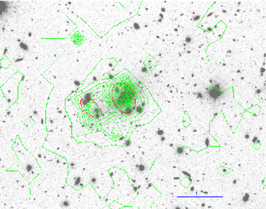
Figure 2.14: Optical image of ABCG 209 with, superimposed, the X–ray contour levels of the Chandra image, with North at top and East to left. The ellipses represent the two substructures detected by Wavdetect. The primary X–ray peak coincides with the position of the cD galaxy and thus with the peak of the bright galaxy distribution (cf. Fig. 2.13 left lower panel). The secondary X–ray peak coincides with the main peak of the faint galaxy distribution (cf. Fig. 2.13 right lower panel).

The X–ray analysis of ABCG 209 was performed by using the Chandra ACIS–I observation 800030 (exposure ID#522) stored in the Chandra archive. The pointing has an exposure time of 10 ksec.

Data reduction was performed by using the package CIAO(Chandra Interactive Analysis of Observations). First, we removed events from the level 2 event list with a status not equal to zero and with grades one, five and seven. Then, we selected all events with energy between 0.3 and 10 keV. In addition, we cleaned bad offsets and examined the data on a chip by chip basis, filtering out bad columns and removing times when the count rate exceeded three standard deviations from the mean count rate per 3.3 second interval. We then cleaned each chip for flickering pixels, i.e. times where a pixel had events in two sequential 3.3 second intervals. The resulting exposure time for the reduced data is 9.86 ks.

The temperature of the ICM was computed extracting the spectrum of the cluster within a circular aperture of 3 arcminutes radius around the cluster center. Freezing the absorbing galactic hydrogen column density at 1.64 10²⁰ cm^-2, computed from the HI maps by Dickey & Lockman (1990), we fitted a Raymond–Smith spectrum using the CIAO package Sherpa with a $\chi^{2}$ statistics. We found a best fitting temperature of $\mathrm{T_{X}=10.2^{+1.4}_{-1.2}}$ keV.

In order to detect possible substructures in ABCG 209 we ran the task CIAO/Wavdetect on a subimage of 1600 by 1600 pixels containing the cluster. The task was run on different scales in order to search for substructure with different sizes. The significance threshold was set at $10^{-6}$.

The results are shown in Fig. 2.14. Two ellipses are plotted representing two significant substructures found by Wavdetect. The principal one, located at $\alpha$= 01 31 52.7 and $\delta$= -13 36 41, is centered on the cD galaxy, the left one is a secondary structure located at $\alpha$= 01 31 55.7 and $\delta$= -13 36 54, about 50 arcseconds ($\sim$120 $\mathrm{h^{-1}}$ kpc) East of the cD (cf. also Fig. 2.13). The secondary clump is well coincident with the Eastern clump detected by Rizza et al. (1998) by using ROSAT HRI X–ray data, while we do not find any significant substructure corresponding to their Western excess.

2.6 Formation and evolution of ABCG 209

The value we obtained for the LOS velocity dispersion $\mathrm{\sigma_{v}\sim 1400}$ km s${}^{-1}\;$(Sect. 2.4.1) is high compared to the typical, although similar values are sometimes found in clusters at intermediate redshifts (cf. Fadda et al. 1996; Mazure et al. 1996; Girardi & Mezzetti 2001). In Sect. 2.4.2 we show that this high value of $\mathrm{\sigma_{v}}$ is not due to obvious interlopers: also a very restrictive application of the “shifting gapper” or the rejection of minor peaks in galaxy density lead to only a slightly smaller value of $\mathrm{\sigma_{v}\sim 1250}$ km s^-1. The high global value of $\mathrm{\sigma_{v}=1250}$–$1400$ km s${}^{-1}\;$is consistent with the high value of $\mathrm{T_{X}\sim 10}$ keV coming from the X–ray analysis (which, assuming $\mathrm{\beta_{spec}=1}$, would correspond to $\mathrm{\sigma_{v}\sim 1300}$ km s${}^{-1}\;$, cf. Fig. 2.2) and with the high value of $\mathrm{L_{X}(0.1-2.4\ keV)\sim 14\;h_{50}^{-2}\;10^{44}}$ erg $\mathrm{s^{-1}}$ (Ebeling et al. 1996; cf. with $\mathrm{L_{X}}$–$\mathrm{\sigma_{v}}$ relation by e.g., Wu et al. 1999; Girardi & Mezzetti 2001).

Therefore, on the basis of the global properties only, one could assume that ABCG 209 is not far from dynamical equilibrium and rely on large virial mass estimate here computed $\mathrm{M(<1.78}$ $\mathrm{h^{-1}}$ Mpc$)=2.25^{+0.63}_{-0.65}\times 10^{15}$ $\mathrm{h^{-1}\ M_{\odot}\;}$or $\mathrm{M(<1.59}$ $\mathrm{h^{-1}}$ Mpc$)=1.62^{+0.48}_{-0.46}\times 10^{15}$ $\mathrm{h^{-1}\ M_{\odot}\;}$.

On the other hand, the analysis of the integral velocity dispersion profile shows that a high value of $\mathrm{\sigma_{v}}$ is already reached within the central cluster region of 0.2–0.3 $\mathrm{h^{-1}}$ Mpc. This suggests the possibility that a mix of clumps at different mean velocity causes the high value of the velocity dispersion.

A deeper analysis shows that ABCG 209 is currently undergoing a dynamical evolution. We find evidence for a preferential SE–NW direction as indicated by: a) the presence of a velocity gradient; b) the elongation in the spatial distribution of the colour–selected likely cluster members; c) the elongation of the X–ray contour levels in the Chandra image; d) the elongation of the cD galaxy.

In particular, velocity gradients are rarely found in clusters (e.g., den Hartog & Katgert 1996) and could be produced by rotation, by presence of internal substructures, and by presence of other structures on larger scales such as nearby clusters, surrounding superclusters, or filaments (e.g., West 1994; Praton & Schneider 1994).

The elongation of the cD galaxies, aligned along the major axis of the cluster and of the surrounding LSS (e.g., Binggeli 1982; Dantas et al. 1997; Durret et al. 1998), can be explained if BCMs form by coalescence of the central brightest galaxies of the merging subclusters (Johnstone et al. 1991).

Other evidence that this cluster is far from dynamical equilibrium comes out from deviation of velocity distribution from Gaussian, spatial and kinematical segregation of members with different B–R colour, and evidence of substructure as given by the Dressler–Schectman test (1988). In particular, although a difference in $\mathrm{\sigma_{v}}$ between blue and red members is common in all clusters (e.g., Carlberg et al. 1997b), a displacement in mean velocity or in position center is more probably associated with a situation of non equilibrium (e.g., Bruzendorf & Meusinger 1999).

Possible subclumps, if any, cannot be easily separated by using 112 cluster members only. The separation in three clumps by using one–dimensional KMM test and the visual inspection of Dressler–Schectman map of Fig. 2.7 represent only two tentative approaches (cf. Sects. 2.4.3 and 2.4.5).

A further step in the detection of possible subclumps is achieved by using the two–dimensional complete sample of all $\sim 400$ colour–selected cluster members. In fact, several clumps appear well aligned in the SE–NW direction, and, in particular, the main clump revealed by faint galaxies (R$>19.5$ mag) coincides with the secondary X–ray peak as found in our analysis of Chandra data (cf. also Rizza et al. 1998). This result suggests that one or several minor clumps are merging along the SE–NW direction, with a main clump hosting the cD galaxy. In particular, the presence of a significant velocity gradient suggests that the merging plane is not parallel to the plane of the sky.

The presence of a secondary clump as a well distinct unit in X–ray data suggests that this clump and maybe the whole cluster might be in a pre–merger phase.

The strong luminosity segregation found for colour–selected galaxies could however suggests a possible alternative dynamical scenario. In fact, very appealingly, galaxies of different luminosity could trace the dynamics of cluster mergers in a different way. A first evidence was given by Biviano et al. (1996): they found that the two central dominant galaxies of the Coma cluster are surrounded by luminous galaxies, accompanied by the two main X–ray peaks, while the distribution of faint galaxies tend to form a structure not centered with one of the two dominant galaxies, but rather coincident with a secondary peak detected in X–ray. The observational scenario of ABCG 209 has some similarities with the situation of Coma: bright galaxies (R$<19.5$ mag) are concentrated around the cD galaxy, which coincides with the primary X–ray peak, while faint galaxies (R$>19.5$ mag) show several peaks, the main of which, Eastern with respect the cD galaxy, is confirmed by the position of the secondary X–ray peak. Therefore, following Biviano et al., we might speculate that the merging is in an advanced phase, where faint galaxies trace the forming structure of the cluster, while more luminous galaxies still trace the remnant of the core–halo structure of a pre–merging clump, which could be so dense to survive for a long time after the merging (as suggested by numerical simulations González–Casado et al. 1994). An extended Radio–emission would support an advanced merging phase, but its presence is still uncertain due to the existence of strong discrete sources (Giovannini et al. 1999). The comparison of present Radio–image with our galaxy distribution shows that the diffuse source is located around the central cD galaxy with an extension toward North.

Unfortunately, redshift data are available only for luminous galaxies and we cannot investigate the nature of subclumps inferred from the two–dimensional distribution of faint galaxies. At the same time, available X–ray data are not deep enough to look for possible variations of temperature in the region of interest.

2.7 Summary

In order to study the internal dynamics of the rich galaxy cluster ABCG 209, we obtained spectra for 159 objects in the cluster region based on MOS observations carried out at the ESO New Technology Telescope. Out of these spectra, we analysed 119 galaxies: 112 turn out to be cluster members, 1 is foreground and 6 are background galaxies.

ABCG 209 appears as a well isolated peak in the redshift distribution centered at $z=0.209$, characterized by a very high value of the LOS velocity dispersion: $\mathrm{\sigma_{v}=1250}$–$1400$ km s^-1, that results in a virial mass of $\mathrm{M=1.6}$–$2.2\times 10^{15}$$\mathrm{h^{-1}\ M_{\odot}\;}$within R_vir. The analysis of the velocity dispersion profile show that such high value of $\mathrm{\sigma_{v}}$ is already reached in the central cluster region ($<0.2$–0.3 $\mathrm{h^{-1}}$ Mpc).

The main results of the present study may be summarised as follows.

• ABCG 209 is characterised by a preferential SE–NW direction as indicated by: a) the presence of a velocity gradient in the velocity field; b) the elongation in the spatial distribution of colour–selected likely cluster members; c) the elongation of the X–ray contour levels in the Chandra image; d) the elongation of the cD galaxy.

• We find significant deviations of velocity distribution from Gaussian.

• Red and blue members are spatially and kinematically segregated.

• There is significant evidence of substructure, as shown by the Dressler & Schectman test.

• The two–dimensional distribution of the colour–selected likely members shows a strong luminosity segregation: bright galaxies $\mathrm{R<19.5}$ are centered around the cD galaxy, while faint galaxies $\mathrm{R>19.5}$ show some clumps. The main one, Eastern with respect to the cD galaxy, is well coincident with the secondary X–ray peak.

This observational scenario suggests that ABCG 209 is presently undergoing strong dynamical evolution. Present results suggest the merging of two or more subclumps along the SE–NW direction in a plane which is not parallel to the plane of sky, but cannot discriminate between two alternative pictures. The merging might be in a very early dynamical status, where clumps are still in the pre–merging phase, or in a more advanced status, where luminous galaxies trace the remnant of the core–halo structure of a pre–merging clump hosting the cD galaxy.

Chapter 3 Luminosity function

In this chapter we derive the luminosity functions in three bands (BVR) for ABCG 209. The data cover an area of $\sim$ 78 arcmin² in the B and R bands, while a mosaic of three pointings was obtained in the V band, covering an area of approximately 160 arcmin². The galaxy sample is complete to B = 22.8 ($\mathrm{N_{gal}}$ = 339), V = 22.5 ($\mathrm{N_{gal}}$ = 1078) and R = 22.0 ($\mathrm{N_{gal}}$ = 679). Although the fit of a single Schechter function cannot be rejected in any band, the luminosity functions are better described by a sum of two Schechter functions for bright and faint galaxies, respectively. There is an indication for a presence of a dip in the luminosity functions in the range V = 20.5–21.5 and R = 20.0–21.0. We find a marked luminosity segregation, in the sense that the number ratio of bright–to–faint galaxies decreases by a factor 4 from the center to outer regions. Our analysis supports the idea that ABCG 209 is an evolved cluster, resulting from the merger of two or more sub–clusters.

3.1 Introduction

Galaxy luminosity function (LF) is a powerful tool to constrain galaxy formation and evolution, since it is directly related to the galaxy mass function and hence to the spectrum of initial perturbations. Hierarchical clustering models predict a mass distribution characterised by a cut–off above a given mass M^∗ and well described by a power law at low masses (Press & Schechter 1974). Starting from these results Schechter (1976) analysed the luminosity distribution of 14 galaxy clusters observed by Oemler (1974), by introducing an analytical description in the form:

$$\mathrm{\phi(L)dL=\phi^{*}\left(\frac{L}{L^{*}}\right)^{\alpha}e^{-\left(\frac{L}{L^{*}}\right)}d\left(\frac{L}{L^{*}}\right)\ .}$$ (3.1)

In the Schechter function $\phi^{*}$ is a normalization density and the shape of the LF is described by L^∗, a characteristic cut–off luminosity, and $\alpha$, the faint–end slope of the distribution. He used this function to describe the global LF of all galaxy types and suggested the value $\alpha=-5/4$.

Although investigated in several works, the universality of the LF faint–end slope is still controversial. The value of the faint–end slope turns out to be $\alpha\sim-1$ for field galaxies (e.g., Efstathiou et al. 1988; Loveday et al. 1992), while clusters and groups seem to have steeper slopes, -1.8 $<\alpha<$ -1.3 (e.g., De Propris et al. 1995; Lumsden et al. 1997; Valotto et al. 1997), suggesting the presence of a larger number of dwarf galaxies (but see also e.g., Lugger 1986; Colless 1989; Trentham 1998). Changes in the slope of the faint–end of the LF in clusters can be related to environmental effects. An increase of the steepening of the LF faint–end in the cluster outer regions was actually observed (Andreon 2001) and explained taking into account that the various dynamical processes which can destroy dwarf galaxies act preferentially in the higher–density cores.

Lopez–Cruz et al. (1997) showed that clusters with a flat LF ($\alpha\sim-1$) are a homogeneous class of rich clusters with a single dominant galaxy, symmetrical single peaked X–ray emission and high gas masses. Irregular clusters have a steeper faint–end, in particular, the LFs of ABCG 1569 and Coma which present substructures, can be suitably fitted with the sum of two Schechter functions with $\alpha=-1$ and $\alpha\geq-1.4$ (Lopez–Cruz et al. 1997). Trentham (1997) also suggested that the faint–end slope of the LF flattens as clusters evolve because of the destruction of dwarf galaxies by merging with giants galaxies.

The density of the environment seems to affect the distribution of galaxy luminosity in the sense that Schechter fits are poor for galaxies in dense environment, where there is an indication of a dip (e.g., Driver et al. 1994; Biviano et al. 1995; Wilson et al. 1997; Molinari et al. 1998; Garilli et al. 1999; N$\mathrm{\ddot{a}}$slund et al. 2000; Yagi et al. 2002). Trentham & Hodgking (2002) identified two types of galaxy LF, one for dynamically evolved regions (i.e. region with a high elliptical galaxy fraction, a high galaxy density, and a short crossing time), such as Virgo cluster and Coma cluster, and one for unevolved regions, such as the Ursa Major cluster and the Local Group. A dip is present in the LF of Virgo and Coma and is absent in LFs of Ursa Major and Local Group.

The differences in shape of the LFs from cluster to cluster could be explained assuming that the total LF is the sum of type specific luminosity functions (hereafter TSLFs), each with its universal shape for a specific type of galaxies (Binggeli et al. 1988). The total LF then assumes a final shape which can be different from cluster to cluster according to the mixture of different galaxy types.

Therefore, different mixtures of galaxies, induced by cluster–related processes, may be at the origin of the presence and of the different shape of dips seen in cluster LFs and may be responsible for the differences seen in the total LFs among field, groups and galaxy clusters.

Indeed, dips are found in several clusters, occurring roughly at the same absolute magnitude (M$\mathrm{{}_{R,dip}}\sim$ -19.4 or $\sim$ M^∗ + 2.5), within a range of about one magnitude, suggesting that clusters have comparable galaxy population. However the dips may have different shapes, and also depend on the cluster region. This could be related to the relative abundances of galaxy types, which depend on the global properties of each cluster and on the local density (Durret et al. 1999).

In order to further investigate the cluster dynamical state, and to discriminate between the pictures, presented in the previous chapter, we derived the LFs by using new photometric data for ABCG 209 based on ESO–NTT imaging in the B, V and R wavebands. The new photometric data are presented in Sect. 3.2. In Sect. 3.3 we describe the data reduction, and the photometric calibrations. The aperture photometry is presented in Sect.3.4, whereas Sect. 3.5 deals with the LFs and Sect. 3.6 with the spatial distribution of galaxies of different luminosity. Sect. 3.7 is dedicated to the summary and the discussion of the results. In this work we assume H₀ = 70 km s${}^{-1}\;$Mpc, $\Omega_{m}$ = 0.3, $\Omega_{\Lambda}$ = 0.7. According to this cosmology, 1 arcmin corresponds to 0.205 Mpc at z = 0.209.

3.2 Observations

Figure 3.1: Area covered by the photometry in the region of ABCG 209. All the galaxies brighter than V = 21.5 are marked with crosses. The central field (solid contour) was observed in B, V and R bands, while the two adjacent fields (dashed contours) were observed only in V band. Circles mark the regions analysed in Sect. 3.6.1. North is up and East is on the left. The origin of the coordinates coincides with the cluster center ($\alpha_{2000}$ = 01 31 52.7, $\delta_{2000}$ = -13 36 41.9). A region around a bright star was not considered in the analysis (right bottom corner of central field).

A field of $9.2^{\prime}\times 8.6^{\prime}$ (1.9 $\times$ 1.8 $\mathrm{h^{-2}_{70}}$ Mpc²), was observed in the B, V and R bands around the cluster center. In order to sample the cluster at large distance from the center, we observed other two fields in V band. The total observed area in V band, accounting for overlapping, is $\sim 160$ arcmin² and is shown in Fig. 3.1. The relevant information on the photometry are summarized in Table 3.1. Standard stars from Landolt (1992) were also observed before and after the scientific exposures, and were used for the photometric calibration.

Table 3.1: Information on the photometric observations.

$$\begin{array}[]{c c c c}\hline\cr\vskip 3.0pt plus 1.0pt minus 1.0pt\cr\mathrm{Band}&\mathrm{T_{exp}}&\mathrm{Seeing}&\mathrm{Scale}\\ &\mathrm{ks}&\mathrm{arcsec}&\mathrm{arcsec/pxl}\\ \vskip 3.0pt plus 1.0pt minus 1.0pt\cr\hline\cr\vskip 3.0pt plus 1.0pt minus 1.0pt\cr\mathrm{B}&1.8&0.80&0.267\\ \mathrm{V}&1.26\times 3&0.80&0.267\\ \mathrm{R}&0.9&0.90&0.267\\ \vskip 3.0pt plus 1.0pt minus 1.0pt\cr\hline\cr\end{array}$$

3.3 Data reduction and photometric calibration

Standard procedures were employed for bias subtraction, flat–field correction, and cosmic ray rejection using the IRAF  package. For each waveband the flat–field was obtained by combining twilight sky exposures. After bias subtraction and flat–field correction the images were combined using the IRAF task IMCOMBINE with the CRREJECT algorithm. Residual cosmic rays and hot pixels were interpolated applying the IRAF task COSMICRAYS. The resulting images show a uniform background with typical r.m.s. of 2.3%, 1.4%, and 1.1% for the B, V, and R bands, respectively.

Table 3.2: Results of the photometric calibration of BVR data.

$$\begin{array}[]{c c c c c c}\hline\cr\vskip 3.0pt plus 1.0pt minus 1.0pt\cr\mathrm{Band}&\mathrm{C}&\gamma&\mathrm{A}&\mathrm{ZP}&\sigma\\ \vskip 3.0pt plus 1.0pt minus 1.0pt\cr\hline\cr\vskip 3.0pt plus 1.0pt minus 1.0pt\cr\mathrm{B}&\mathrm{B-V}&-0.037\pm 0.008&0.322\pm 0.010&24.885\pm 0.015&0.016\\ \mathrm{V}&\mathrm{B-V}&0.035\pm 0.009&0.204\pm 0.013&25.277\pm 0.021&0.020\\ \mathrm{R}&\mathrm{V-R}&0.010\pm 0.017&0.145\pm 0.014&25.346\pm 0.023&0.026\\ \vskip 3.0pt plus 1.0pt minus 1.0pt\cr\hline\cr\end{array}$$

The photometric calibration was performed into the Johnson–Kron–Cousins photometric system by using the Landolt standard fields. The instrumental magnitudes of the stars were measured in a fixed aperture by using the IRAF packages APPHOT and DAOPHOT. The aperture size was chosen in order to i) enclose the total flux, ii) obtain the maximum signal–to–noise ratio. By comparing the magnitudes of the stars in different apertures, we found that a reasonable compromise is achieved with an aperture of radius 10 pixels (cf. Howell 1989). For each band, we adopted the following calibration relation:

$$\mathrm{M}=\mathrm{M^{{}^{\prime}}}+\gamma\cdot\mathrm{C}-\mathrm{A}\cdot\mathrm{X}+\mathrm{ZP}\ ,$$ (3.2)

where M and C are the magnitudes and colours of the standard stars, M${}^{{}^{\prime}}$ is the instrumental magnitude, $\gamma$ is the coefficient of the colour term, A is the extinction coefficient, X is the airmass and ZP is the zero–point. The quantities $\gamma$, A and ZP were derived by a least square procedure with the IRAF task FITPARAMS. The results of the photometric calibrations are reported in Table 3.2. Unless otherwise stated, errors on estimated quantities are given at 68% confidence level (hereafter c.l.).

As a test we compare the (B–R, V–R) diagram of the Landolt standard stars with that of the stars in the cluster field. We measured the magnitude of these stars by using the software SExtractor (Bertin & Arnouts 1996). We verified that the observed distribution of stars in our images matches that of the Landolt stars in the (B–R, B–V) plane, proving the accuracy of the photometric calibration.

3.4 Aperture photometry

For each image, a photometric catalog was derived by using the software SExtractor (Bertin & Arnouts 1996). We measured magnitudes within a fixed aperture of 5.0${}^{{}^{\prime\prime}}$, corresponding to $\sim$ 17 kpc at z = 0.209, and Kron magnitudes (Kron 1980), for which we used an adaptive aperture with diameter $a\cdot r_{K}$, where $r_{K}$ is the Kron radius and $a$ is a constant. We chose $a$ = 2.5, yielding $\sim$ 94% of the total source flux within the adaptive aperture (Bertin & Arnouts 1996). The aperture magnitudes were used in order to derive galaxy colours. The different seeing of the R–band image introduces a systematic shift, indipendent from the total magnitude, of $\sim$ 0.03 mag, that is smaller than the photometric errors on colours. The measured magnitudes were corrected for galactic extinction following Schlegel et al. (1998). The uncertainties on the magnitudes were obtained by adding in quadrature both the uncertainties estimated by SExtractor and the uncertainties on the photometric calibrations.

Figure 3.2: Completeness magnitudes of the B–, V–, and R–band images are estimated by comparing magnitudes in the fixed aperture (M_ap) and in the detection cell (M_cell). The dotted lines represent the completeness limits, the dashed lines mark the limits in the detection cell, and solid lines are the linear relations between M_ap and M_cell.

The completeness magnitudes were derived following the method of Garilli et al. (1999), as shown in Fig. 3.2. We estimated the completeness magnitude as the magnitude where galaxies start to be lost because they are fainter than the brightness threshold in the detection cell. The completeness magnitudes are B_C = 22.8 (N_gal = 339), V_C = 22.5 (N_gal = 1078), and R_C = 22.0 (N_gal = 679).

In order to derive the LF we considered the objects brighter than the completeness limit and adopted the Kron magnitude, since this is the best estimate of the total magnitude. The star/galaxy classification was based on the SExtractor stellar index (SG), defining as stars the sources with SG $\geq$ 0.98.

By examination of the distribution of sources classified as stars and galaxies in the magnitude-FWHM plane, and the number-magnitude distribution of sources classified as stars, we believe the classification to be efficient up to the completeness magnitude of the catalogues, where stars constitutes $\sim 12.5$% of all sources.

Figure 3.3: Number–magnitude distribution of sources classified by SExtractor as stars. The continuous line represents the best–fitting power–law function to the counts for 19.0$<$ R $<$ 21.5.

Figure 3.3 shows the number-magnitude distribution of sources classified as stars by SExtractor in the R–band. For 19.0$<$ R $<$ 21.5 the distribution behaves as a power–law as would be expected (see Groenewegen et al. 2002). By extrapolating the power–law to magnitude R = 22.0, we estimate that the level of contamination by stars in the range 21.5–22.0 is minimal ($\sim$ 4 stars in the whole observed area).

The catalogs for the central region of the cluster were cross–correlated by using the IRAF task XYXYMATCH. For each object, colours were derived within the fixed aperture.

3.5 Luminosity Functions

In order to measure the cluster LF in each band we used all the galaxy photometric data up to the completeness magnitude, and removed the interlopers by statistically subtracting the background contamination. We used galaxy counts in B, V and R bands from the ESO–Sculptor Survey (Arnouts et al. 1997; de Lapparent et al. 2003) kindly provided to us by V. de Lapparent. These data cover an area of $\sim$ 729 arcmin² observed with EMMI instrument. The data reduction was performed by using the procedures similar to those adopted in the present work. In particular, the photometric catalog was obtained by SExtractor and the total magnitudes were estimated from the Kron magnitudes defined by adopting the same aperture.

We assumed Poisson statistics for the background and cluster field galaxy counts. The errors on the cluster LFs were computed by adding in quadrature Poissonian fluctuations. Fluctuation of background galaxy counts are no simply Poissonian, besause of the galaxy correlation function. The galaxy counts variance due to the angular correlation function, for each bin of magnitude, can be estimated by using Eq. (5) in Huang et al. 1997. By using this formula, we verify that the background fluctuations do not influence our estimate of the best-fit parameters of the luminosity function and the errors on this parameters (there is only a change of 0.1% in the confidence levels). The errors on the cluster LFs are dominated by Poissonian errors on observed counts, since the field of view of our observations corresponds to an area with equivalent radius of $\sim$ 1 Mpc $h_{70}^{-1}$, that is 10 times smaller than the area covered by the background counts and 7 times smaller than the scale of the angular correlation function.

We derived the LFs for the central field (see Fig. 3.1) in the B, V and R bands by fitting the galaxies counts with a single Schechter function. In V and R bands the fits were also computed with the sum of two Schechter functions in order to describe the bright and the faint populations (Sect. 3.5.1). We compared the LFs with counts obtained selecting red sequence galaxies (Sect. 3.5.2). All the fit parameters and the $\chi^{2}$ statistics, are listed in Table 3.3.

3.5.1 Multiband analysis

Figure 3.4 (solid lines) shows the LFs in the B, V and R bands for the central cluster region, obtained by a weighted parametric fit of the Schechter function to the statistically background–subtracted galaxy counts (filled circles). The parameters of the fit are: B^∗ = 20.06, $\mathrm{\alpha_{B}}$ = -1.26, V^∗ = 18.29, $\mathrm{\alpha_{V}}$ = -1.27, R^∗ = 17.78, $\mathrm{\alpha_{R}}$ = -1.20. We evaluated the quality of the fits by means of the $\chi^{2}$ statistics (see Table 3.3). The single Schechter function gives a fair representation of the global distribution of the data, that is the single Schechter fit cannot be rejected in any band even at the $10\%$ c.l. .

Table 3.3: Fits to the Luminosity Functions. Errors on the $\mathrm{M^{*}}$ and $\alpha$ parameters can be obtained by the confidence contours shown in Fig. 3.4.

$$\begin{array}[]{c| c c c c| c c c c }\hline\cr\vskip 3.0pt plus 1.0pt minus 1.0pt\cr\mathrm{Band}&\lx@intercol\hfil\mathrm{\leavevmode\nobreak\ \leavevmode\nobreak\ \leavevmode\nobreak\ \leavevmode\nobreak\ \leavevmode\nobreak\ Single\leavevmode\nobreak\ Schechter\leavevmode\nobreak\ function}\nobreak\leavevmode\nobreak\leavevmode\nobreak\leavevmode\nobreak\leavevmode\nobreak\leavevmode\hfil\lx@intercol\vrule\lx@intercol&\lx@intercol\hfil\mathrm{\leavevmode\nobreak\ \leavevmode\nobreak\ \leavevmode\nobreak\ \leavevmode\nobreak\ \leavevmode\nobreak\ Two\leavevmode\nobreak\ Schechter\leavevmode\nobreak\ functions^{(a)}\leavevmode\nobreak\ }\hfil\lx@intercol\\ \vskip 3.0pt plus 1.0pt minus 1.0pt\cr\hline\cr\vskip 3.0pt plus 1.0pt minus 1.0pt\cr&\leavevmode\nobreak\ \leavevmode\nobreak\ \leavevmode\nobreak\ \leavevmode\nobreak\ \leavevmode\nobreak\ \leavevmode\nobreak\ \mathrm{M^{*}}\nobreak\leavevmode\nobreak\leavevmode\nobreak\leavevmode\nobreak\leavevmode\nobreak\leavevmode\nobreak\leavevmode&\leavevmode\nobreak\ \leavevmode\nobreak\ \leavevmode\nobreak\ \leavevmode\nobreak\ \alpha\nobreak\leavevmode\nobreak\leavevmode\nobreak\leavevmode\nobreak\leavevmode&\leavevmode\nobreak\ \leavevmode\nobreak\ \leavevmode\nobreak\ \leavevmode\nobreak\ \leavevmode\nobreak\ \mathrm{\chi^{2(b)}_{\nu}}\nobreak\leavevmode\nobreak\leavevmode\nobreak\leavevmode\nobreak\leavevmode\nobreak\leavevmode&\mathrm{P(\chi^{2}>\chi^{2}_{\nu})}\nobreak\leavevmode&\leavevmode\nobreak\ \leavevmode\nobreak\ \leavevmode\nobreak\ \mathrm{M}^{*}_{faint}\nobreak\leavevmode\nobreak\leavevmode\nobreak\leavevmode&\leavevmode\nobreak\ \leavevmode\nobreak\ \alpha_{faint}\nobreak\leavevmode\nobreak\leavevmode&\leavevmode\nobreak\ \leavevmode\nobreak\ \leavevmode\nobreak\ \mathrm{\chi^{2}_{\nu}}\nobreak\leavevmode\nobreak\leavevmode\nobreak\leavevmode&\mathrm{P(\chi^{2}>\chi^{2}_{\nu})}\\ \vskip 3.0pt plus 1.0pt minus 1.0pt\cr\hline\cr\vskip 3.0pt plus 1.0pt minus 1.0pt\cr\mathrm{B}&-21.03&-1.26&0.96&46\%&&&&\\ \mathrm{V^{c}}&-22.03&-1.25&1.04&40\%&&&&\\ \mathrm{V}&-22.18&-1.27&1.46&15\%&-18.72&-2.00&1.09&37\%\\ \mathrm{R}&-22.48&-1.20&1.24&27\%&-19.14&-1.24&1.06&39\%\\ \vskip 3.0pt plus 1.0pt minus 1.0pt\cr\hline\cr\vskip 3.0pt plus 1.0pt minus 1.0pt\cr\lx@intercol\hfil\mathrm{}\hfil\lx@intercol&\lx@intercol\hfil\mathrm{\leavevmode\nobreak\ \leavevmode\nobreak\ \leavevmode\nobreak\ \leavevmode\nobreak\ \leavevmode\nobreak\ Galaxies\leavevmode\nobreak\ on\leavevmode\nobreak\ the\leavevmode\nobreak\ red\leavevmode\nobreak\ sequence}\nobreak\leavevmode\nobreak\leavevmode\nobreak\leavevmode\nobreak\leavevmode\nobreak\leavevmode\hfil\lx@intercol&\lx@intercol\hfil\hfil\lx@intercol\\ \vskip 3.0pt plus 1.0pt minus 1.0pt\cr\hline\cr\mathrm{V}&-22.60&-1.33&2.10&2\%&-18.68&-2.19&1.68&9\%\\ \mathrm{R}&-22.76&-1.27&1.30&23\%&-19.15&-1.39&1.09&37\%\\ \vskip 3.0pt plus 1.0pt minus 1.0pt\cr\hline\cr\end{array}$$

• The bright–end LF is fixed (see text).

• The reduced $\mathrm{\chi^{2}}$.

• Total observed field (see Sect. 3.6).

On the other hand, there is indication of a dip in the distribution at V $\sim$ 21.0 and R $\sim$ 20.5. According to the fitted single Schechter function, there should be 121 and 125 galaxies in the range V = 20.5–21.5 and R = 20.0–21.0 respectively, whereas in our counts we find $\sim 92\pm 10$ and $\sim 105\pm 10$ galaxies. If we define the dip amplitude as:

$$\mathrm{A=\frac{N_{e}-N_{o}}{N_{e}}\ ,}$$ (3.3)

where $\mathrm{N_{e}}$ and $\mathrm{N_{o}}$ are the expected and observed number of galaxies in the dip magnitude range, we obtain in V (R) band A$=24\pm 8\%$ ($16\pm 8\%$). The position of dips are: M_V $\sim$ -19.5 and M_R $\sim$ -19.8. These values were obtained by converting apparent into absolute magnitudes using k–corrections for early–type galaxies from Poggianti (1997). The B–band data are not deep enough to sample the dip position.

Figure 3.4: Luminosity function in the B, V and R bands in the central field of 9.2${}^{\prime}\times$ 8.6^′. In V and R bands filled circles represent counts obtained from the photometric catalog with a statistical background subtraction, open circles are the counts of galaxies belonging to the red sequence of the CM relation (see Sect. 3.5.2). Solid and dashed lines are the Schechter fits to the filled and open circles respectively. In the small panels the 1, 2 and 3$\sigma$ c.l. of the best–fit parameters $\alpha$ and M^∗ are shown.

The presence of a dip was discussed in the literature by considering the properties of the TSLFs (e.g., Binggeli et al. 1988) in nearby clusters. In a study of the Virgo cluster, Sandage et al. (1985) showed the presence of two distinct classes of galaxies (normal and dwarfs), with different dynamical and luminosity evolution. Since the bright–end of the LF is well studied, we can use a priori the information about the LF shape for bright galaxies to fit our data with two different Schechter functions, representing bright and faint galaxies. We assumed a Schechter model with R${}^{*}\mathrm{{}_{bright}}$ = 18.0 and $\alpha\mathrm{{}_{R,bright}}$ = -1.0 (from N$\mathrm{\ddot{a}}$slund et al. 2000 results, scaled according to the adopted cosmology). Using the V–R colour term as derived from Eq. (3.4), we also fix V${}^{*}\mathrm{{}_{bright}}$ = 18.7 and $\alpha\mathrm{{}_{V,bright}}$ = -1.0.

Figure 3.5 shows the cluster LFs in V and R bands modelled with the two Schechter functions. The fit procedures yields V${}^{*}\mathrm{{}_{faint}}$ = 21.75, R${}^{*}\mathrm{{}_{faint}}$ = 21.12. For the slope of the faint galaxies function the V– and R–band data provide poor constraints, so that we have only an indication of a steep faint–end. According to the $\chi^{2}$ statistics (see Table 3.3), combining two Schechter functions for bright and faint galaxies the quality of the fit increases both in V and R bands.

Figure 3.5: Luminosity function in the V and R bands in the central field of 9.2${}^{\prime}\times$ 8.6^′. The dashed lines represent the Schechter functions for bright and faint galaxies separately (see text). The continuous line represents the sum of the two functions. In the small panels the 1, 2 and 3$\sigma$ c.l. of the best–fit parameters $\alpha$ and M^∗ are shown.

3.5.2 Galaxies on the red sequence

We obtained the Colour–Magnitude (CM) relation by fitting the photometric data of the spectroscopically confirmed cluster members (see Chapter 2) with a biweight algorithm (Beers et al. 1990):

$$\mathrm{(V-R)_{CM}=-0.023\cdot R+1.117\ .}$$ (3.4)

By using Eq. (3.4), we defined as sequence galaxies the sources lying in the region inside the curves:

$$\mathrm{(V-R)_{seq}=(V-R)_{CM}\pm(\sqrt{\sigma_{V}^{2}+\sigma_{R}^{2}}+0.05)\ ,}$$ (3.5)

where we took into account the photometric uncertainty at 1$\sigma$ both on the V ($\mathrm{\sigma_{V}}$) and on the R magnitude ($\mathrm{\sigma_{R}}$) as well as the intrinsic dispersion of the CM relation (Moretti et al. 1999). In Fig. 3.6 the red sequence galaxies are marked with filled circles.

Figure 3.6: V–R vs. R CM diagram for all the galaxies within the completeness limit in the central field of ABCG 209. Galaxies of the red sequence (see solid line) are plotted as filled circles. The solid line defines the CM sequence for spectroscopically confirmed cluster members.

By selecting galaxies on the CMR (within the observed scatter), the background contamination is expected to be negligible. So we can directly compare galaxy counts (open circles in Fig. 3.4) with those derived in Sect. 3.5.1 (filled circles in Fig. 3.4). In both V and R bands the counts obtained with the two different approaches are very similar.

Figure 3.4 (dashed lines) shows the LFs in the V and R bands for the central cluster region, obtained by a weighted parametric fit of the Schechter function to the red galaxy counts (open circles). The parameters of the fit are: V^∗ = 17.87, $\mathrm{\alpha_{V}}$ = -1.33, R^∗ = 17.50, $\mathrm{\alpha_{R}}$ = -1.27. According to the $\chi^{2}$ statistics (see Table 3.3) we can reject the fit with a single Schechter function in the V band at 98% c.l. At the same time, the dip amplitude in the V band, A$=26\pm 9\%$, is unchanged respect to the case of the global LF (Sect. 3.5.1). It turns out that, independently from the fitted Schechter functions, the ratio ($\sim 60\%$) of observed counts in the bins inside the dip and in the bins adjacent to the dip regions is the same for both galaxy samples, while the overall distribution of red galaxies cannot be described with a single Schechter function. According to the $\chi^{2}$ statistics (see Table 3.3), combining two Schechter functions the quality of the fit increases both in V and R bands, and becomes acceptable also in the V band.

3.6 Luminosity segregation

The data in the V band, covering an area of $\sim$ 160 arcmin², corresponding to a circular region with equivalent radius 0.6 R_vir (R_vir = 2.5 h${}^{-1}_{70}$ Mpc; see Sect. 2.4.1), allow to study the environmental dependence of LF and the spatial distribution of galaxies as a function of the clustercentric distance.

Figure 3.7 (upper panel) shows the V–band LF in the whole observed area, modelled by using a weighted parametric fit to a single Schechter function, with best fit values V^∗ = 18.45 (M$\mathrm{{}^{*}_{V}}$ = -22.03) and $\mathrm{\alpha_{V}}$ = -1.25. The LF shape is very similar to that obtained in the central field (Fig. 3.4) and also in this case the Schechter function overestimates the observed counts in the range V = 20.5–21.5. The dip amplitude is A$=14\pm 7\%$.

3.6.1 The LF in different cluster regions

Table 3.4: Best fit value of the LFs measured in three regions around the center of the cluster.

$$\begin{array}[]{c c c c c c }\hline\cr\vskip 3.0pt plus 1.0pt minus 1.0pt\cr\mathrm{Region}&\mathrm{Area(h^{-2}_{70}Mpc^{2})}&\mathrm{V}^{*}&\mathrm{Luminosity\ ratio}&\mathrm{\chi^{2}_{\nu}}&\mathrm{P(\chi^{2}>\chi^{2}_{\nu})}\\ \vskip 3.0pt plus 1.0pt minus 1.0pt\cr\hline\cr\vskip 3.0pt plus 1.0pt minus 1.0pt\cr\mathrm{A}&0.50&18.09\pm 0.73&12.7\pm 3.0&1.12&35\%\\ \mathrm{B}&1.00&18.49\pm 0.44&6.9\pm 1.4&1.08&37\%\\ \mathrm{C}&1.00&18.88\pm 0.43&6.8\pm 2.3&0.85&56\%\\ \vskip 3.0pt plus 1.0pt minus 1.0pt\cr\hline\cr\end{array}$$

In order to compare the abundances of galaxies of various luminosities in different regions we computed the LFs in three areas at different distances from the center . First we considered the cluster counts in an area of 0.5 h${}^{-2}_{70}$ Mpc² around the center of the cluster (region A), and then in two concentric circular rings around the first central region, each in an area of 1.0 h${}^{-2}_{70}$ Mpc², respectively at $\sim$ 2^′ and $\sim$ 4.7^′ from the center (region B and C). We fitted the counts using a single Schechter function with $\alpha$ fixed at the best fit value obtained from the LF computed over the whole observed field. Table 3.4 reports the relative fit values in the different regions and Fig. 3.7 shows the fitted functions. We also measured the luminosity weighted ratio of the number of objects brighter and fainter than the V = 21.0 (Table 3.4), that is the magnitude where the dip occurs. This luminosity ratio increases from region B to the center by a factor $1.8\pm 0.6$, indicating a significant luminosity segregation, whereas the ratio does not vary from the region B to the region C.

Figure 3.7: Luminosity function in the V band. In the upper panel are shown the LF in the whole observed area (160 arcmin²) and the 1, 2 and 3$\sigma$ c.l. of the best–fit parameters $\alpha$ and M^∗ (small panel). The continuous line represents the fitted Schechter functions. In the other panels the LFs in the three cluster regions (see text) are shown. Continuous lines are the fit of the Schechter functions obtained by fixing the faint–end slope at the best fit value of the LF fitted on the whole observed area.

3.6.2 Spatial distribution of galaxies

In Fig. 3.8 (left panel) the number density radial profile is shown, i.e. the number of galaxies measured in concentric rings around the center. It has been computed for the whole galaxy population (open circles) and for galaxies brighter (filled circles) and fainter (triangles) than V = 21.0, the magnitude where the luminosity distribution shows the distinctive upturn. The number of faint galaxies is determined up to the completeness limit. The densities are statistically background–subtracted by using background galaxy density measured in the ESO–Sculptor Survey (Arnouts et al. 1997). Errors are assumed to be Poissonian.

Figure 3.8: The background–subtracted radial profile of ABCG 209 is shown in the left panel. Open circles represent the distribution of all galaxies in the cluster, filled circles are bright galaxies (M$\mathrm{{}^{*}_{V}\leq}$ -19.5) and open triangles are faint galaxies (M$\mathrm{{}^{*}_{V}>}$ -19.5). The number of bright galaxies in the first and in the second bin is $\sim$ 32 and $\sim$ 17 respectively, while the number of faint galaxies is $\sim$ 15 and $\sim$ 30. The bright–to–faint ratio as a function of the clustercentric distance is shown in the right panel.

The radial profile of all galaxies is centrally peaked, showing the highest gradient for bright galaxies (Fig. 3.8, left panel). Indeed, the bright galaxy density decreases by a factor $\sim 5.4$ between the first and the second bin, to be compared with a decrease of a factor $\sim 1.4$ for faint galaxies and of a factor $\sim 2.6$ when all galaxies are considered. For faint galaxies (V $>$ 21.0), the distribution decreases slowly with clustercentric distance.

Fig. 3.8 (right panel) shows the bright–to–faint ratio (BFR) as a function of the clustercentric distance. The BFR shows a maximum at the center, where the number of bright galaxies is two times the number of faint galaxies, and decreases rapidly between the first and the second bin. Outside the central region of the cluster (r $>$ 1 arcmin) the BFR distribution is flat and there are roughly two faint galaxies for each bright galaxy.

3.7 Summary and discussion

The analysis performed on ABCG 209 can be summarized by the following results:

1)

the fit with a single Schechter function cannot be rejected in any band; at the same time, the luminosity distributions are better described by a sum of two Schechter functions for bright and for faint galaxies respectively;

2)

there is an indication of a dip in V– and R–band LFs, and this features is also present when considering only galaxies that lie on the red sequence;

3)

the faint–end slope seems to be steeper going from redder to bluer wavelengths;

4)

there is a luminosity segregation, in the sense that the V^∗ value increases from the center to the outer regions and the luminosity ratio of bright–to–faint galaxies decreases by a factor $\sim 2$ from the center to outer regions, whereas the number ratio decreases by a factor $\sim 4$.

The presence of a dip was found in the LF of many clusters. In Table 3.5 we reported the positions of the dips for some of these clusters with 0.0$<$ z $<$ 0.3 in R–band absolute magnitudes (according to the adopted cosmology). The literature data were transformed to R–band absolute magnitudes by using k– and evolutionary correction, and average colours for early–type galaxies of Poggianti (1997).

Table 3.5: Compilation of dip positions in the restframe R band in cluster LFs from literature. Data were transformed to R–band absolute magnitudes by using k– and evolutionary correction, and average colours for early–type galaxies of Poggianti (1997).

$$\begin{array}[]{c c c c }\hline\cr\vskip 3.0pt plus 1.0pt minus 1.0pt\cr\mathrm{Cluster\ name}&\mathrm{Redshift}&\mathrm{\leavevmode\nobreak\ \leavevmode\nobreak\ \leavevmode\nobreak\ \leavevmode\nobreak\ Dip\ position}&\mathrm{Reference}\\ \vskip 3.0pt plus 1.0pt minus 1.0pt\cr\hline\cr\vskip 3.0pt plus 1.0pt minus 1.0pt\cr\mathrm{Virgo}&0.0040&-18.9&\mathrm{Sandage\ et\ al.(1985)}\\ \mathrm{ABCG\,194}&0.018&-19.8&\mathrm{Yagi\ et\ al.(2002)}\\ \mathrm{Coma}&0.0232&-19.8&\mathrm{Biviano\ et\ al.(1995)}\\ \mathrm{ABCG\,496}&0.0331&-19.8&\mathrm{Durret\ et\ al.(2000)}\\ \mathrm{ABCG\,2063}&0.035&-19.3&\mathrm{Yagi\ et\ al.(2002)}\\ \mathrm{ABCG\,576}&0.038&-18.6&\mathrm{Mohr\ et\ al.(1996)}\\ \mathrm{Shapley8}&0.0482&-19.5&\mathrm{Metcalfe\ et\ al.(1994)}\\ \mathrm{ABCG\,754}&0.053&-19.3&\mathrm{Yagi\ et\ al.(2002)}\\ \mathrm{ABCG\,85(z)}^{\mathrm{a}}&0.0555&-19.9&\mathrm{Durret\ et\ al.(1999)}\\ \mathrm{ABCG\,85}&0.0555&-19.3&\mathrm{Durret\ et\ al.(1999)}\\ \mathrm{ABCG\,2670}&0.076&-19.3&\mathrm{Yagi\ et\ al.(2002)}\\ \mathrm{ABCG\,1689}&0.181&-18.7&\mathrm{Wilson\ et\ al.(1997)}\\ \mathrm{ABCG\,665}&0.182&-18.7&\mathrm{Wilson\ et\ al.(1997)}\\ \mathrm{ABCG\,963}&0.206&-19.0&\mathrm{Driver\ et\ al.(1994)}\\ \mathrm{ABCG\,209}&0.209&-19.6&\mathrm{This\,work}\\ \mathrm{MS\,2255.7+2039}&0.288&-19.6&\mathrm{N\ddot{a}slund\ et\ al.\ (2000)}\\ \vskip 3.0pt plus 1.0pt minus 1.0pt\cr\hline\cr\end{array}$$

• LF fitted only on the spectroscopically confirmed cluster galaxies.

Dips are found at comparable absolute magnitudes, in different clusters, suggesting that these clusters may have similar galaxy population. However, the dips have not necessarily the same shape: the dips found in the the LF of Shapley 8 and Coma are broader than those found in Virgo, ABCG 963, and ABCG 85. As already mentioned in the introduction, this can be explained with the hypothesis of an universal TSLF (Binggeli et al. 1988), whereas the different relative abundances of galaxy types, induced by cluster–related processes, are at the origin of the different dip shapes (see also Andreon 1998).

Moreover, as shown in Table 3.5, there is no correlation between the dip position and the redshift, suggesting little or no evolutionary effect in the dip, in agreement with N$\mathrm{\ddot{a}}$slund et al. (2000), which directly compare the LFs of Coma, ABCG 963 and MS2255. They detected no qualitative difference between nearby and distant clusters.

Studying the R–band LFs for a photometric sample of 10 clusters at different redshifts and with different richness classes, Yagi et al. (2002) demonstrated that the dips seen in the LFs are almost entirely due to r^1/4–like galaxies. This evidence is in agreement with those shown in Fig. 3.4 (open circles). In fact by comparing the counts of red sequence galaxies with those obtained with a statistical background subtraction, the dip in V band appears more pronounced.

Environmental effects can be at the origin of the different positions of the dips seen in different clusters, since the transition from the bright–dominated to the faint–dominated parts of the LF can occur at different magnitudes in different environment. The cluster morphological mix and the morphology–density relation (Dressler 1980) should give rise to LFs with different shape when subdividing a sample galaxies respect to the cluster environments.

The effect of the environment can be seen in ABCG 209 by comparing the shape of the LF in V band in different regions around the cluster center (see Fig. 3.7 and Sect. 3.6.1). The fitted M^∗ value is shifted toward fainter magnitudes going from the inner (A) to the outer (C) region and the luminosity ratio of bright–to–faint galaxies decreases by a factor $\sim 2$, indicating a luminosity segregation.

The bright galaxies are markedly segregated in the inner 0.2 h${}^{-1}_{70}$, around the cD galaxy. This suggest that bright galaxies could trace the remnant of the core–halo structure of a pre–merging clump.

Although ABCG 209 is a cD–like cluster, with cD galaxy located in the center of a main X–ray peak, it shows an elongation and asymmetry in the galaxy distribution (Chapter 2). Moreover, the faint–end slope turns out to be $\alpha<-1$ at more than 3$\sigma$ c.l. in both V and R bands, thus reconciling the asymmetric properties of X–ray emission with the non flat–LF shape of irregular systems as found by Lopez–Cruz et al. (1997).

These results allow to discriminate between the two possible formation scenarios suggested by the dynamical analysis (Chapter 2). We conclude that ABCG 209 is an evolved cluster, resulting from the merger of two or more sub–clusters, while the elongation and asymmetry of the galaxy distribution (of the X–ray emission) and the shape of the LFs show that ABCG 209 is not yet a fully relaxed system.

Our analysis is in agreement with the existence of i) an universal LF for bright galaxies, which is well described by a flat Schechter function, and ii) a steep Schechter function for faint galaxies. A definitive conclusion regarding the faint–end slope of the LF needs deeper photometry able to sample the luminosity distribution of dwarf galaxies.

Chapter 4 Galaxy evolution in different environments

In this chapter we examine the environmental effects on the photometric properties of galaxies for the rich galaxy cluster ABCG 209 at $z=0.209$. We use archive CFHT optical imaging of a $42\times 28\,{\rm arcmin}^{2}$ field centred on the cluster to produce a galaxy sample complete to $B=25.0$ and $R=24.5$. Both the composite and red sequence galaxy luminosity functions are found to be dependent on the local galaxy surface density, their faint-end slopes becoming shallower with increasing density. We explain this as a combination of the morphology-density relation, and dwarf galaxies being cannibalised and/or disrupted by the cD galaxy and the ICM in the cluster core. The $B-R$ colour of the red sequence itself appears 0.02 mag redder for the highest-density regions, indicative of their stellar populations being marginally ($<5$%) older or ($<20$%) more metal-rich. This may be due to the galaxies themselves forming earliest in the rarest overdensities marked by rich clusters, or their star formation being suppressed earliest by the ICM.

4.1 Introduction

The effect of local environment on the formation and evolution of galaxies is one of the most pressing issues in cosmology today, with evidence that environmental processes affect the mass distribution of galaxies, as well as their star formation and morphological characteristics. Rich clusters provide a unique opportunity to study these environmental effects, providing large numbers of galaxies at the same redshift which have been exposed to a wide variety of environments. Numerous authors have studied the environmental effects of rich clusters on the luminosity functions, star formation rates and morphologies of the constituent galaxies (e.g. Lopez–Cruz et al. 1997; Balogh, Navarro & Morris 2000; Hogg et al. 2003; Treu et al. 2003).

The galaxy luminosity function (LF), which describes the number of galaxies per unit volume as a function of luminosity, is a powerful tool for examining galaxy formation and evolution, since it can be directly related to the galaxy mass function. The Press-Schechter prescription for the hierarchical assembly of galaxies predicts a simple analytical formula for the mass distribution of the form ${\rm n(M)dM}\propto{\rm M}^{\alpha}\exp(-{\rm M/M}^{*})$ (Press & Schechter 1974) which reproduces well the results of N-body simulations of the growth of dark matter halos. This relation was confirmed by the observations of Schechter (1976), that also suggested that the shape of the galaxy LF is universal, and only the multiplicative constant $\psi^{*}$ differs between clusters.

Numerous studies have since been made to determine the galaxy LF: some confirming the validity of the “universal luminosity function hypothesis” (e.g. Lugger 1986; Colless 1989; Trentham 1998); whereas others indicate that the LF is instead dependent on the environment of the galaxies, resulting in significant differences between the LFs from cluster to cluster and between cluster and field (e.g. Lopez–Cruz et al. 1997; Valotto et al. 1997). More recent studies, based on large surveys, empirically suggest that the galaxy LF is indeed dependent on environment, with dynamically-evolved, rich clusters and clusters with central dominant galaxies having brighter characteristic luminosities and shallower faint-end slopes than poorer clusters (Lopez–Cruz et al. 1997; De Propris et al. 2003). In particular these differences can be explained by considering the composite LF as the sum of type-specific luminosity functions (TSLFs), each with its universal shape for a specific type of galaxies (e.g. ellipticals, spirals, dwarfs). The shape of the composite LF can then vary from cluster to cluster, and from clusters to field, according to the mixture of different galaxy types in each environment resulting from the morphology-density relation (Dressler et al. 1987; Binggeli et al. 1988).

The galaxies most synonymous with the cluster environment are the bulge-dominated, passively-evolving galaxies which make up the cluster red sequence. Studies of low-redshift clusters (e.g. Bower, Lucey & Ellis 1992) indicate that, irrespective of the richness or morphology of the cluster, all clusters have red sequences, whose k-corrected slopes, scatters and colours are indistinguishable. Other studies find similar regularities between other physical properties of the early-type galaxies (surface-brightness, mass-to-light ratio, radius, velocity distribution, metallicity) resulting in the Faber-Jackson (Faber & Jackson 1976) and Kormendy (1977) relations and the fundamental plane (Djorgovski & Davis 1987; Dressler et al. 1987). These all indicate that the early-type galaxies which make up the red sequences form a homogeneous population, not only within each cluster, but from cluster to cluster, and also that red sequences are universal and homogeneous features of galaxy clusters, at least at $z\mathrel{\hbox{\hbox to0.0pt{\hbox{\lower 4.0pt\hbox{$\sim$}}\hss}\hbox{$<$}}}0.2$.

The photometric evolution of the cluster red sequence with redshift has been studied by a number of authors (e.g. Aragón-Salamanca et al. 1993; Ellis et al. 1997; Stanford et al. 1998; Kodama et al. 1998) for clusters out to $z\simeq 1.2$ indicating i) that the red sequence remains a universal feature of clusters; ii) that the stellar populations of its constituent early-type galaxies are formed in a single, short burst at an early epoch $(z_{f}\mathrel{\hbox{\hbox to0.0pt{\hbox{\lower 4.0pt\hbox{$\sim$}}\hss}\hbox{$>$}}}2)$; and iii) that the galaxy colours have evolved passively ever since. This is confirmed by the spectra of red-sequence galaxies which, in nearby clusters, are best fit by simple stellar populations of age 9–12 Gyr, resulting in those galaxies having characteristically strong spectral breaks at 4000 Å, and correspondingly red $U-V$ colours.

Cosmological models of structure formation indicate that the densest regions of the universe, corresponding to the rarest overdensities in the primordial density field, have collapsed earliest, and contain the most massive objects, i.e. rich galaxy clusters. Detailed cosmological simulations which follow the formation and evolution of galaxies (e.g. Kauffmann 1996; Blanton et al. 2000) predict that galaxies in these high-density regions are older and more luminous than those in typical density (i.e. field) regions. Having initially ($z\sim 5$) been the most likely place for the formation of stars and galaxies, the high-density environment of rich cluster cores is later ($z\sim$1–2) filled with shock-heated virialised gas that does not easily cool and collapse (Blanton et al. 1999), inhibiting both the formation of stars and galaxies (Blanton et al. 2000), which instead occurs most efficiently in increasingly less massive dark matter halos. These models are able to successfully predict the observed cluster-centric star formation and colour gradients, and the morphology-density relation of $z<0.5$ clusters (Balogh et al. 2000; Diaferio et al. 2001; Springel et al. 2001; Okamoto & Nagashima 2003), although it is not clear whether they predict trends with density of colour or star formation for galaxies of a fixed morphology and luminosity. They show that these gradients in galaxy properties naturally arise in hierarchical models, because mixing is incomplete during cluster assembly, and the positions of galaxies within the clusters are correlated with the epoch at which they were accreted.

To examine the effect of environment on galaxy properties, in particular the galaxy luminosity function, and the cluster red sequence, we have performed a photometric study of the galaxy cluster ABCG 209 using archive wide-field $B$ and $R$-band imaging, which allows the photometric properties of the cluster galaxies to be followed out to radii of 3–4$h_{70}^{-1}$ Mpc.

The cluster was initially chosen for its richness, allowing its internal velocity field and dynamical properties to be studied in great detail, and also for its known substructure, allowing the effect of cluster dynamics and evolution on the properties of its member galaxies to be examined. All the results presented in previous chapters indicate that ABCG 209 is undergoing strong dynamic evolution with the merging of two or more sub-clumps along the SE-NW direction. This dynamical situation is confirmed by the weak lensing analysis of Dahle et al. (2002) which shows the cluster to be highly elongated in the N-S direction, and two significant peaks, the largest being coincident with the cluster centre and cD galaxy, and the second separated by 6 arcmin in the north direction.

The photometric data are presented in Section 4.2. As this cluster has been found to be significantly elongated along the SE-NW direction, we examine the effect of the cluster environment by measuring galaxy properties as a function of local surface density rather than cluster-centric radius. We describe the method for determining the cluster environment in Sect. 4.3. The ability to successfully subtract the background field population is vital to study the global properties of cluster galaxies from photometric data alone, and we describe the approach to this problem in Sect. 4.4. The composite galaxy LF is presented in Sect. 4.5, and the properties of the red sequence galaxies described in Sect. 4.6. The effects of environment on the blue galaxy fraction and mean galaxy colours are presented in Sects. 4.7 and 4.8. Sect. 4.9 is dedicated to the summary and discussion of the results. In this work we assume H₀=70 km s^-1 Mpc^-1, $\Omega_{m}=0.3$, and $\Omega_{\Lambda}=0.7$. In this cosmology, the lookback time to the cluster ABCG 209 at $z=0.209$ is 2.5 Gyr.

4.2 The data

The data were obtained from the Canada-France-Hawaii telescope (CFHT) science archive (PI. J.-P. Kneib), comprising wide-field $B$- and $R$-band imaging centred on the cluster ABCG 209. The observations were made on 14–16 November 1999, using the CFHT12K mosaic camera, an instrument made up of 12 $4096\times 2048$ CCDs, set at the prime focus of the 3.6-m CFHT. The CCDs have a pixel scale of $0.206^{\prime\prime}$, resulting in a total field of view of $42\times 28\,{\rm arcmin}^{2}$, corresponding to $8.6\times 5.7\,h^{-2}_{70}{\rm Mpc}^{2}$ at the cluster redshift. The total exposure times for both $B$- and $R$-band images are 7 200s, made up of eight 900s $B$-band and twelve 600s $R$-band exposures, jittered to cover the gaps between the CCDs.

Standard procedures were used to bias-subtract the images, using bias exposures and the overscan regions of each CCD. Saturated pixels and bleed trails from bright stars are identified and interpolated across. The images were then flat-fielded using a superflat made up of science images taken using the same camera/filter setup of cluster ABCG 209, as well as those of the clusters A 68, A 383, A 963, CL 0818 and CL 0819 which were also observed as part of the same observing program. For each image, the sky is subtracted by fitting a quadratic surface to each CCD. The sky is then modelled using a $256\times 256$ pixel median filter, rejecting all pixels $>3\sigma$ from the median (i.e. galaxies).

Cosmic rays are removed by comparison of each image with a registered reference image (taken to be the previous exposure). After masking off those pixels $3\sigma$ above the median in the reference image (taken to be sources) each pixel which has a value $3\sigma$ higher than its value in the reference image, is flagged as a cosmic ray and interpolated across. The individual images are corrected for airmass using the prescribed values from the CFHT website of $\alpha(B)=-0.17$ and $\alpha(R)=-0.06$. The photometry of non-saturated guide stars is found to agree between exposures to an rms level of 0.003 mag, indicating the observations were taken in photometric conditions.

The images are registered and coadded in a two-step process. Each of the 12 CCDs are initially registered and coadded, using the positions of sources from the 2nd Guide Star Catalogue (GSC2) to determine integer-pixel offsets between the jittered exposures. As the exposures are jittered to cover the gaps between the CCDs, there is some overlap between the coadded images of adjacent CCDs. This is used to create linear transforms allowing 12 CCDs to be “stitched” together to form an interim coadded image. This interim image is then used as a reference to which each individual exposure is registered. The registered exposures are then coadded after masking out the gaps between CCDs and bad columns, using $3\sigma$ clipping. The distortion produced by the camera optics is modelled and removed as a quartic-polynomial fit to the positions of GSC2 sources in a reference tangential plane astrometry.

The photometric calibration was performed into the Johnson-Kron-Cousins photometric system using observations of $\sim 300$ secondary standard stars ($14<R<17$) in fields 6 and 7 of Galadí-Enríquez, Trullols & Jordi (2000). The fields also contain equatorial standard stars of Landolt (1992) tying the photometric calibration to the Landolt standards, while allowing the uncertainty of the zeropoint and colour-terms to be reduced and measured in a statistical manner. The median photometric uncertainty for each standard star was $\Delta(B)=0.033$, and $\Delta(R)=0.021$. The zero-points and colour terms were fitted using a weighted least-squares procedure, and are shown in Table 4.1 along with the observed FWHMs of each image.

Band FWHM	Colour	Zeropoint	Colour Term
$B$     1.02	$B-R$	$25.720\pm 0.008$	$-0.0180\pm 0.005$
$R$     0.73	$B-R$	$25.983\pm 0.005$	$\;\;\,0.0002\pm 0.004$

Table 4.1: Photometric parameters of optical data.

Object detection was performed using SExtractor in two-image mode (Bertin & Arnouts 1996) for sources with 4 contiguous pixels 1$\sigma$ over the background level in the $R$-band image. The total $B$ and $R$ magnitudes were taken to be the Kron magnitude, for which we used an adaptive elliptical aperture with equivalent diameter $a.r_{K}$, where $r_{K}$ is the Kron radius, and $a$ is fixed at a constant value of 2.5. $B-R$ colours were determined using fixed apertures of 5 arcsec diameter (corresponding to $\sim 17$ kpc at $z=0.209$), after correcting for the differing seeing of the $R$- and $B$-band images. The measured magnitudes were corrected for galactic extinction following Schlegel, Finkbeiner & Davis (1998) measured as ${\rm E}(B-V)=0.019$, giving ${\rm A}(B)=0.083$ and ${\rm A}(R)=0.051$. The uncertainties in the magnitudes were obtained by adding in quadrature both the uncertainties estimated by SExtractor and the uncertainties of the photometric calibrations.

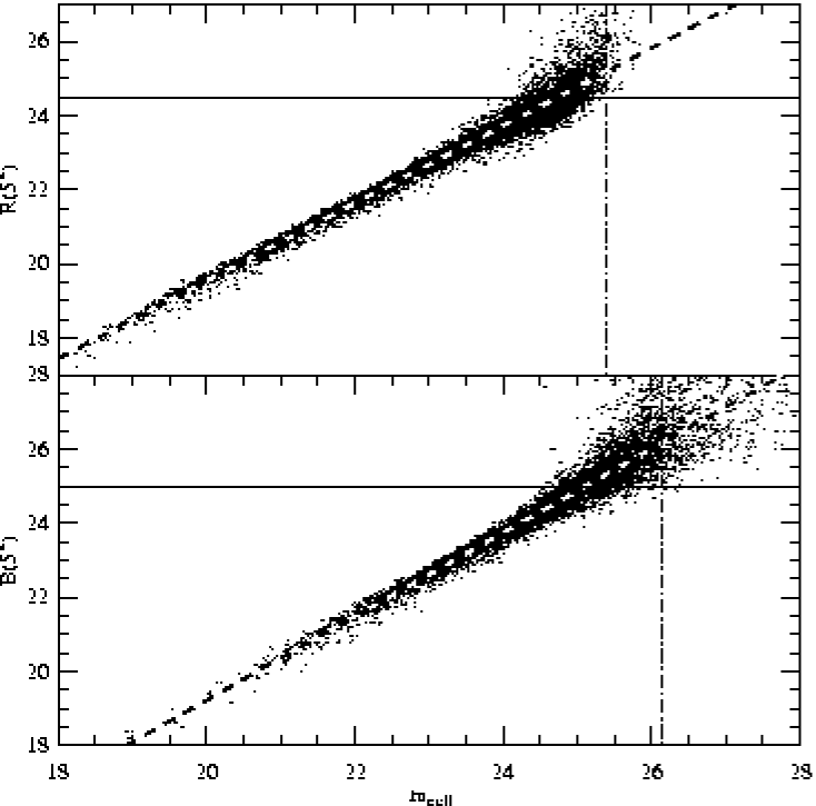
Figure 4.1: Completeness magnitudes of the $B$- and $R$-band images, as estimated by comparing the magnitudes in the fixed aperture (m_ap) and in the detection cell (m_cell). The horizontal solid lines represent the completeness limits, the vertical dot-dashed lines mark the limits in the detection cell, and the dashed lines are the linear relations between m_ap and m_cell.

The completeness magnitudes were derived following the method of Garilli, Maccagni & Andreon (1999), as shown in Fig. 4.1, which compares the magnitudes in the fixed aperture (m_ap) and in the detection cell (m_cell) which in our case is an aperture of area 4 pixels. The magnitude limits at which galaxies are lost due to being fainter than the threshold in the detection cell are determined, and are indicated by the vertical dot-dashed lines. There is a correspondence between $m_{cell}$ and m_ap as shown by the dashed line, which has a certain scatter that depends essentially on the galaxy profile and the photometric errors. To minimise biases due to low-surface brightness galaxies, the completeness magnitude limits are chosen to consider this dispersion, and are indicated by the horizontal solid lines at $B=25.0$ and $R=24.5$. For the analyses of the cluster red sequence, we consider a magnitude limit of $R=23.0$, in order that we remain complete for galaxies with $B-R\sim 2.0$.

4.2.1 Star - Galaxy Separation

Figure 4.2: Photometric properties of sources classified by SExtractor as being stars. (top panel) Number-magnitude distribution of stars. The best-fitting power-law function to the counts for $19<R<22$ is indicated, as is the $R=23$ magnitude limit used for analysis of the red sequence galaxy population. (bottom panel) $B-R$ colour distribution of $19<R<22$ stars, normalised to match the expected level of stellar contamination for $22<R<23$.

Star-galaxy separation is performed using the SExtractor stellarity index, with stars defined as sources with stellarities $\geq 0.98$. By examination of the distributions of sources classified as stars and galaxies in the magnitude-FWHM plane, and the number-magnitude distribution of sources classified as stars, we believe the classification to be efficient to $R\sim 22$ and $B\sim 23$, where stars constitute 12% of all sources.

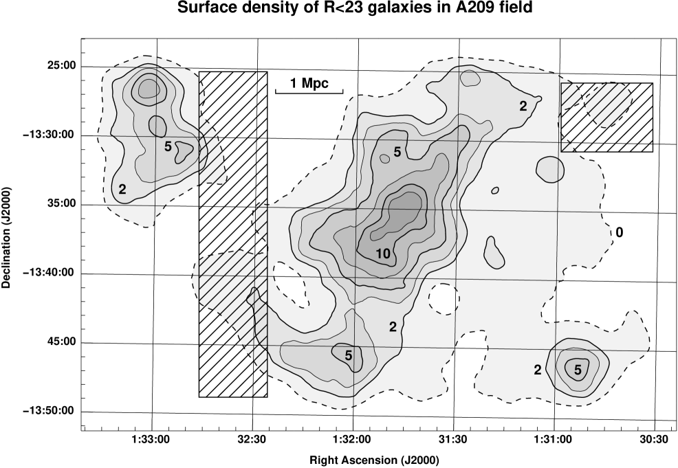
Figure 4.3: The surface density of $R<23.0$ galaxies in the field of ABCG 209. The dashed contour corresponds to the field galaxy number density, while the solid contours correspond respectively to 2, 3.3, 5, 7.5, 10, and 12.5 cluster galaxies arcmin^-2. The shaded boxes indicate the regions used to represent the field galaxy population.

Figure 4.2(top) shows the number-magnitude distribution of sources classified as stars by SExtractor. For $19<R<22$ the distribution behaves as a power-law as would be expected (see Groenewegen et al. 2002). At brighter magnitudes, stars become saturated, while at fainter magnitudes, the classifier begins to misclassify stellar sources as galaxies. By extrapolating the power-law to fainter magnitudes, as indicated by the solid diagonal line, we estimate the level of contamination by stars in the range $22<R<23$ to be $\approx 200$ over the whole field (0.18 stars arcmin^-2), or $\sim 5\%$ of all sources. However, since the contamination from faint stars should affect those regions used to define the field galaxy population at the same level as for the cluster regions, when we correct for field galaxy contamination, the contamination due to faint stars should automatically cancel out also.

Figure 4.2(bottom) shows the $B-R$ colour distribution of stars in the range $19<R<22$. The y-axis is normalised to represent the expected level of contamination by stars in the range $22<R<23$ over the whole field, i.e. 200 in total, assuming the colour distribution remains constant. The distribution is clearly bimodal with two sharp peaks at $B-R\sim 1.0$ and $B-R\sim 2.7$ indicating the dominant populations of white and red dwarf stars (Groenewegen et al. 2002). Fortunately, as regards the study of the red sequence galaxy population of ABCG 209, at these magnitudes the red sequence corresponds approximately to $2.0<B-R<2.2$, midway between the two peaks in the colour distribution of stars. Hence, the expected level of contamination by stars to the red sequence galaxy population is minimal, corresponding to $\sim 6$ stars over the whole mosaic image with $22<R<23$.

4.3 Defining the Cluster Environment

To study the effect of the cluster environment on galaxies in the vicinity of ABCG 209, the local surface density of galaxies, $\Sigma$, is determined across the CFHT images. This is achieved using an adaptive kernel estimator (Pisani 1993; 1996), in which each galaxy is represented by an exponential kernel, $K(r)\propto\exp(-r/r_{0})$, whose width, $r_{0}$ is proportional to $\Sigma^{-1/2}$, thus ensuring greater resolution where it is needed in the high-density regions, and more smoothing in the low-density regions where the signal-to-noise levels are much lower. For this study, the surface number density of $R<23.0$ galaxies is considered, the magnitude limit to which cluster red sequence galaxies can be detected in both passbands. The local density for each galaxy is initially determined using an exponential kernel whose width is fixed to 60 arcsec, and then iteratively recalculated using adaptive kernels, before corrected for field contamination. The resultant surface number density map of the ABCG 209 field is shown in Fig. 4.3. The dashed contour corresponds to the density of field galaxies, while the thick contours correspond to 2, 5 and 10  cluster galaxies arcmin^-2, the densities used to separate the three cluster environments described below.

The spatial distribution shows the complex structure of this cluster, characterised by the clear elongation in the SE-NW direction (see Chapter 2), indicative of the cluster having gone through a recent merger event. There are also present three other subclumps, the first one about 10 arcmin south along the cluster elongation, the second at about 18 arcmin to the north-east, and the last one, the smallest, at about 18 arcmin to the south-west. The colour information on galaxies in these peaks confirm that these could be groups/clusters at the same redshift as ABCG 209, each peak containing galaxies belonging to the cluster red sequence of ABCG 209. Given the complexity of the structure of ABCG 209, it is important that to study the effect of environment on galaxy properties, we measure them as a function of local galaxy number surface density rather than cluster-centric radius as is usual in these type of studies.

For the following analyses on the effect of the cluster environment on its constituent galaxy population we define three regions selected according to the local surface number density. Firstly we consider a high-density region with $\Sigma>10\,$gals arcmin^-2, which corresponds to the cluster core out to a radius of $\sim$500 kpc, and covers 16.0 arcmin². Next we consider intermediate- ($5<\Sigma<10\,$gals arcmin^-2) and low-density ($2<\Sigma<5\,$gals arcmin^-2) regions which probe the cluster periphery with median galaxy cluster-centric radii of 1.3 and 2.2 Mpc, and cover 68.0 and 189.6 arcmin² respectively. It should be stated that in each case we are studying the cluster galaxy population and not that of the field, and the low-density environment represents an overdense region.

4.4 Statistical Field Galaxy Subtraction

Figure 4.4: The $B-R/R$ colour-magnitude diagrams of the cluster galaxy population in the three cluster regions corresponding to high-, intermediate-, and low-density environments. Each of the three diagrams is the result of a Monte-Carlo realisation in which field galaxies are subtracted statistically. For comparison the C-M diagram of field galaxies is shown also. In each plot the solid line indicates the best-fitting C-M relation of Eq. 4.2, and galaxies identified as belonging to the red sequence through Eq. 4.4 are indicated by solid circles.

To accurately measure the properties of the cluster population as a function of environment requires the foreground / background contamination to be estimated efficiently and corrected. Given the lack of spectroscopic information, we estimate the field galaxy contamination as a function of magnitude and colour (see also Kodama & Bower 2001).

The sample of field galaxies is taken from two regions within the CFHT12K field indicated in Fig. 4.3 by the shaded boxes. These areas were identified as regions where the local galaxy surface density reached a stable minimum level over a wide area indicative of the field. They also have galaxy number counts within $1\sigma$ of the ESO-Sculptor survey of Arnouts et al. (1997) which covers an area of $0.24\times 1.52\,$deg², and is complete to $B=24.5$ and $R=23.5$. The two “field” regions in the ABCG 209 field cover in total 160.9 arcmin², and contain 965 galaxies to $R=23.0$, resulting in a number surface density of 6.0 gals.arcmin^-2, as indicated in Fig. 4.3 by the dashed contour.

A two-dimensional distribution histogram of these field galaxies is built with bins of width 0.25 mag in $B-R$ colour and 0.5 mag in $R$ magnitude. Similar histograms are the constructed for each of the three cluster regions, which also obviously include a field galaxy contamination. The field histogram is normalised to match the area within each cluster region, and for each bin $(i,j)$ the number of field galaxies $N_{i,j}^{field}$ and the cluster plus field $N_{i,j}^{cluster+field}$ are counted. The former can be larger than the latter for low-density bins due to low number statistics, in which case the excess number of field galaxies are redistributed to neighbouring bins with equal weight until $N_{i,j}^{field}<N_{i,j}^{cluster+field}$ is satisfied for all bins. For each galaxy in the cluster region the probability that it belongs to the field is then defined as:

$$P(field)=\frac{N_{i,j}^{field}}{N_{i,j}^{cluster+field}},$$ (4.1)

where the numbers are taken from the bin that the galaxy belongs to. For each cluster region, 100 Monte-Carlo simulations of the cluster population are realised and averaged.

The $B-R/R$ C-M diagrams for Monte-Carlo realisations of the cluster galaxy population for each of the three cluster regions corresponding to high-, intermediate-, and low-density environments are shown in Fig. 4.4, along with that for the field region used for the statistical field subtraction. The different distributions of the cluster and field populations are obvious, with the red sequence prominent in both high- and intermediate-density regions.

4.5 The Galaxy Luminosity Function

Figure 4.5: The $B$- and $R$-band LFs of galaxies in the virial region. The solid curve indicates the best-fitting Schechter function whose parameters are indicated in Table 4.2. In the small panels, the 1, 2 and $3\sigma$ confidence levels of the best-fitting parameters $\alpha$ and $M^{*}$ are shown.

Figure 4.6: The $B$-band LFs of galaxies in the three cluster regions corresponding to high-, intermediate- and low-density environments.

Figure 4.7: The 1, 2 and $3\sigma$ confidence limits for the best-fitting Schechter parameters $\alpha$ and $B^{*}$ for the three cluster regions corresponding to low- (solid contours), intermediate- (dotted) and high-density (dashed) environments.

Figure 4.8: The $R$-band LFs of galaxies in the three cluster regions corresponding to high-, intermediate- and low-density environments.

Figure 4.9: Confidence limits for the best-fitting Schechter parameters $\alpha$ and $R^{*}$ for the three cluster regions. Contours as for Fig. 4.7.

In order to measure the cluster LF in each band we used all the galaxy photometric data up to the completeness magnitudes and removed the interlopers by statistically subtracting the background contamination, as determined from the two field regions. The errors on the cluster LFs are computed by adding in quadrature the Poisson fluctuations for the galaxy counts in both the cluster and field regions, and fluctuations due to photometric errors on Kron magnitudes.

We compute the cluster LFs for both $B$ and $R$ bands for galaxies within one virial radius, and examine the effect of the cluster environment by determining the LFs for each of the three cluster regions corresponding to high-, intermediate- and low-density environments. For each cluster LF, we fit the observed galaxy counts with a single Schechter function. Absolute magnitudes are determined using the k-corrections for early-type galaxies from Poggianti (1997). All the fit parameters and associated $\chi^{2}$ statistics are listed in Table 4.2.

	Region	$B^{*}$	M∗	$\alpha$	$\chi^{2}_{\nu}$
$\!\!B\!\!$	$r<{\rm R}_{vir}$	20.01	-21.07	-1.28	0.59
$\!\!B\!\!$	$\Sigma>10$	20.60	-20.48	-1.11	0.61
$\!\!B\!\!$	$\!5\!<\!\Sigma\!<\!10\!$	20.09	-20.99	-1.38	0.92
$\!\!B\!\!$	$\!2\!<\!\Sigma\!<\!5\!$	19.03	-22.05	-1.50	0.65
	Region	$R^{*}$
$\!\!R\!\!$	$r<{\rm R}_{vir}$	17.71	-22.55	-1.26	1.07
$\!\!R\!\!$	$\Sigma>10$	18.14	-22.12	-1.11	0.85
$\!\!R\!\!$	$\!5\!<\!\Sigma\!<\!10\!$	18.03	-22.23	-1.23	0.88
$\!\!R\!\!$	$\!2\!<\!\Sigma\!<\!5\!$	18.20	-22.06	-1.35	0.66

Table 4.2: Fits to the LFs for cluster galaxies. Errors on the $M^{*}$ and $\alpha$ parameters are indicated by the confidence contours shown in Figures 4.5, 4.7 and 4.9.

4.5.1 Galaxies within the Virial Radius

Figure 4.5 shows the LFs in the $B$ and $R$ bands for galaxies within one virial radius ($2.5h^{-1}_{70}$ Mpc) of the cluster centre. The solid curves show the best-fitting single Schechter functions, obtained by weighted parametric fits to the statistically background-subtracted galaxy counts. According to the $\chi^{2}$ statistic, the global distributions of the data are well described by single Schechter functions, although there is an indication of a dip at $R\sim 20.5$, as already noted in the previous study of the LF in the central region of the cluster (Chapter 3).

In that study, where a smaller area was considered, the amplitude of this dip was calculated by comparing expected and observed counts in the range $R=2$0–21, and found to be ${\rm A}=16\pm 8$%. For galaxies within the virialised region we obtain a value for the dip amplitude of ${\rm A}=32\pm 20$%, which is consistent with that previously obtained.

In Chapter 3 we derived the LFs for the central field of $9.2^{\prime}\times 8.6^{\prime}$ ($1.9\times 1.8h^{-2}_{70}\,{\rm Mpc}^{2}$) by using EMMI–NTT images, complete to $B=22.8$ and $R=22.0$. In this previous study we subtracted statistically the field contamination using background counts in $B$- and $R$-bands from the ESO-Sculptor Survey (Arnouts et al. 1997; de Lapparent et al. 2003). The parameters of the best-fitting Schechter functions were: $B^{*}=20.06$, $\alpha_{B}=-1.26$, and $R^{*}=17.78$, $\alpha_{R}=-1.20$, which are fully consistent with those derived here.

4.5.2 The effect of environment

To examine the effect of environment on the galaxy LF, we have determined the $B$- and $R$-band LFs for galaxies in three regions selected according to their local density. Figures 4.6 and 4.8 show respectively the $B$- and $R$-band LFs in the three different cluster regions, corresponding to high-, intermediate-, and low-density environments. Each LF is modelled through use of a weighted parametric fit to a single Schechter function, the results of which are presented in Table 4.2. measured by fixing $\alpha$ to the value determined for the region within one virial radius, and fitting a Schechter function to the bright end of the galaxy LF ($B<22$ and $R<20$) for each region.

As for the region within one virial radius, the single Schechter function gives a good representation of the global distribution of the data for each cluster environment in both $B$- and $R$-bands. In both high- and low-density regions, no dip is apparent at $R=2$0–21, although the observed counts are marginally below that predicted from the Schechter function. Only in the intermediate-density region is a significant dip apparent, where a deficit of $R=20.$0–20.5 galaxies significant at the $2\sigma$ level is observed with respect to the fitted Schechter function.

Figures 4.7 and 4.9 show the confidence contours for the best fitting Schechter functions for $\alpha$ and $B^{*}$, and $\alpha$ and $R^{*}$ respectively, for each of the three cluster regions, allowing the trends with density to be followed. In both $B$ and $R$ bands, the faint-end slope becomes significantly steeper from high- to low-density environments, the values of $\alpha$ determined for the high- and low-density regions being inconsistent at more than the $3\sigma$ confidence level.

4.6 Properties of the Red Sequence Galaxies

We determined the colour-magnitude (CM) relation of galaxies in the cluster ABCG 209 by averaging over 100 Monte-Carlo realisations of the cluster population, and fitting the resultant photometric data of the $\sim 480$ $R<21$ galaxies within one virial radius with the biweight algorithm of Beers et al. (1990) obtaining

$$(B-R)_{CM}=3.867\pm 0.006-0.0815\pm 0.0098\times R.$$ (4.2)

Here the errors quoted consider the uncertainty due to background subtraction, photometric errors, and uncertainty from the fitting itself as measured using the scale value of the biweight algorithm. The $B-R$ colour dispersion around the red sequence is measured as a function of magnitude, $\sigma(R)$, for galaxies in each magnitude bin over the range $18<R<23$. It is found to be consistent with being due to an intrinsic colour dispersion, $\sigma_{int}$ and the photometric error, $\sigma_{B-R}^{2}(R)$ added in quadrature,

$$\sigma(R)^{2}=\sigma_{int}^{2}+\sigma_{B-R}^{2}(R).$$ (4.3)

The intrinsic dispersion around the red sequence is found to be $\sigma_{int}=0.10$ mag, which is much higher than the dispersion level of 0.05 mag found for the Coma and Virgo clusters (Bower, Lucey & Ellis 1992), and which is often quoted as being typical for low redshift rich clusters. However, in a similar study of the $B-R/R$ CM-relation for 11 $0.07<z<0.16$ clusters Pimbblet et al. (2002) obtain typical dispersion levels of 0.06–0.08, and observe three clusters with dispersion levels higher than ours.

Using this equation, we then defined those galaxies lying within the region between the curves:

$$(B-R)_{\pm}=(B-R)_{CM}\pm\sqrt{\sigma^{2}_{int}+\sigma^{2}_{B-R}}$$ (4.4)

as being red sequence galaxies.

As for the composite luminosity function, we determine the $R$-band luminosity function of red sequence galaxies within one virial radius of the cluster centre, as shown in Figure 4.10.

Figure 4.10: The $R$-band LF of red sequence galaxies in the virial region. The solid curve indicates the best-fitting Schechter function whose parameters are indicated in the top-left of each plot. In the small panels, the 1, 2 and $3\sigma$ confidence levels of the best-fitting parameters $\alpha$ and $R^{*}$ are shown.

Figure 4.11: The $R$-band LFs of red sequence galaxies in the three cluster regions corresponding to high-, intermediate- and low-density environments. The solid curve indicates the best-fitting Schechter function whose parameters are indicated in the top-left of each plot.

Figure 4.12: Confidence limits for the best-fitting Schechter parameters $\alpha$ and $R^{*}$ for the three cluster regions. Contours as for Fig. 4.7.

4.6.1 The effect of environment on the C-M relation

We also determine the C-M relation in the high- and intermediate-density regions separately, to see if there is any environmental effect on the relation. By fixing the slope at -0.0815, we find the red sequence to be $0.022\pm 0.014$ mag redder in the high-density region than for the intermediate-density region. The effect of environment on the red sequence slope was also examined by leaving the slope as a free parameter, but no significant change was observed. It was not possible to extend this analysis to the low-density region, as the red sequence was poorly constrained due to a much larger contamination by outliers.

The $R$-band luminosity functions of red sequence galaxies (as selected according to Eq. 4.4) in each of the three cluster environments is shown in Figure 4.11, and the best fitting parameters shown in Table 4.3. The solid curve shows the best-fitting Schechter function found through a maximum likelihood analysis whose parameters $\alpha$ and $R^{*}$ are indicated in the top-left of each plot. The errors for each bin are determined as the uncertainty from the field galaxy subtraction and the Poisson noise due to galaxy counts in the cluster and field regions, all added in quadrature.

Region	$R^{*}$	$M^{*}$	$\alpha$	$\chi_{\nu}^{2}$
$r<{\rm R}_{vir}$	17.94	-22.22	-1.08	1.61
$\Sigma>10$	18.04	-22.30	-0.97	0.95
$5<\Sigma<10$	17.94	-22.20	-1.00	0.45
$2<\Sigma<5$	17.90	-22.24	-1.15	0.90

Table 4.3: Fits to the red sequence galaxy LFs. Errors on the $R^{*}$ and $\alpha$ parameters are indicated by the confidence contours shown in Figs. 4.10 and 4.12.

For the cluster red sequence we consider a magnitude limit of $R=23.0$. At this magnitude, red sequence galaxies have $B-R\sim 2.0$, and so are at the completeness limit of the $B$-band image, and have typical uncertainties of $\Delta(R)\sim 0.06$ and $\Delta(B-R)\sim 0.11$. As discussed earlier, the expected contamination of stars is minimal due to their colour-distribution, and for the three cluster regions corresponding to high-, intermediate-, and low-density environments, should be at the level of 0.1, 0.3 and 0.8 stars respectively.

Figure 4.12 shows the confidence contours for the best-fitting Schechter parameters $\alpha$ and $R^{*}$ for each of the three cluster regions, allowing the trends with density to be followed. As for the overall galaxy luminosity function, the $R$-band luminosity function of red sequence galaxies has a steeper faint-end slope, $\alpha$, in the low-density regions than for their high-density counterparts, although the effect here is smaller, and significant only at the $1.7\sigma$ level. Also in each of the three cluster environments, the faint-end slope for the overall galaxy luminosity function is steeper than that for the luminosity function of red sequence galaxies only. This is due to the red sequence galaxies dominating at bright magnitudes, while at faint magnitudes they constitute only $\sim 25\%$ of the cluster population.

4.7 Blue Galaxy Fraction

Figure 4.13: The blue galaxy fraction as a function of local number density.

One of the classic observations of the study of galaxy evolution is the Butcher-Oemler (1984) effect in which the fraction of blue galaxies in clusters is observed to increase with redshift. Here instead we consider the effect of environment on the fraction of blue galaxies. We define the blue galaxy fraction as the fraction of $R<20$ ($\sim$M${}^{*}\!+\!2$) galaxies with rest-frame $B-V$ colours at least 0.2 mag bluer than that of the C-M relation, as for the original studies of Butcher & Oemler (1984). We estimate the corresponding change in $B-R$ colour at the cluster redshift by firstly considering two model galaxies at $z=0$ (Bruzual & Charlot 1993), one chosen to be a typical red-sequence galaxy (10 Gyr old, $\tau=0.1$ Gyr, $Z=0.02$), and the second reduced in age until its $B-V$ colour becomes 0.2 magnitude bluer. After redshifting both galaxies to the cluster redshift, the difference in their observed $B-R$ colour is found to be 0.447 mag. Hence we consider the blue galaxy fraction to be the fraction of $R<20$ galaxies having $B-R<3.420-0.0815\times R$. Figure 4.13 shows the resulting blue galaxy fractions in the high-, intermediate-, and low-density environments after averaging over 100 Monte-Carlo realisations of the cluster population. We find the blue galaxy fractions are low in both the high- ($0.062\pm 0.042$) and intermediate-density ($0.088\pm 0.042$) regions, but increases dramatically to $0.200\pm 0.072$ in the low-density region. Kodama & Bower (2001) examine the dependence of the blue galaxy fraction on radius for 7 clusters at $0.2<z<0.43$, and observe a general trend for $f_{B}$ to increase with radius, the effect becoming more prominent for the higher redshift clusters. For each cluster, the $f_{B}$ in the cluster core ($r\mathrel{\hbox{\hbox to0.0pt{\hbox{\lower 4.0pt\hbox{$\sim$}}\hss}\hbox{$<$}}}0.5$ Mpc), remains low at $\sim 0.10$, whereas at cluster-centric radii of 1–2 Mpc, the $f_{B}$ increases dramatically to 0.2–0.6.

4.8 Galaxy colours

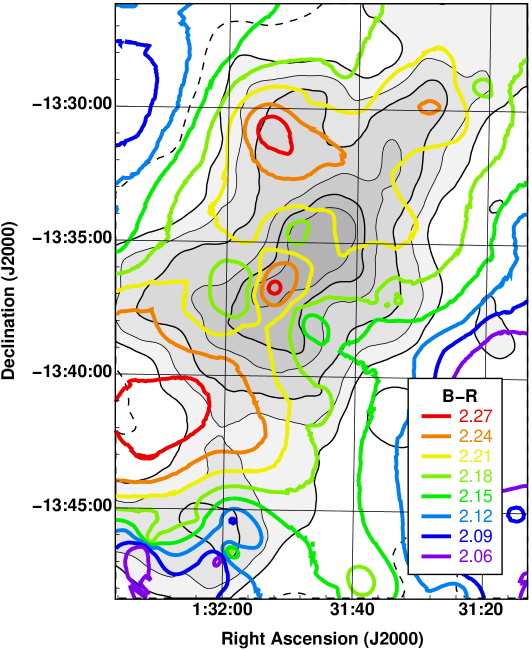
Figure 4.14: The mean galaxy colour of the cluster galaxy population as a function of spatial position (see text).

To gain some further insight into the effect of cluster environment and also the particular dynamical state of ABCG 209, we plot in Figure 4.14 the mean $B-R$ colour of $R<21$ cluster galaxies as a function of spatial position. This is determined as for the surface density map of Fig. 4.3 through the adaptive kernel approach (Pisani 1993; 1996), in which each galaxy is weighted according to the probability that it is a cluster member, $1-P(f)$, so that for a particular point, $\mathbf{x}$, the local mean galaxy colour is given by:

$$\overline{(B\!-\!R)}_{\mathbf{x}}=\frac{\sum_{i=1}^{N}(B\!-\!R)^{CM}_{i}.(1\!-\!P(f)_{i}).K(\mathbf{x}\!-\!\mathbf{x}_{i};r_{i})}{\sum_{i=1}^{N}(1\!-\!P(f)_{i}).K(\mathbf{x}\!-\!\mathbf{x}_{i};r_{i})}$$ (4.5)

where $\mathbf{x}_{i}$, $P(f)_{i}$ and $r_{i}$ are the position, probability of being a field galaxy, and kernel width respectively of galaxy $i$ out of $N$. And $(B-R)_{i}^{CM}$ is the $B-R$ colour for each galaxy after accounting for the luminosity-dependent effect of the slope of the CM-relation through

$$(B-R)_{i}^{CM}=(B-R)_{i}+0.0815\times(R_{i}-19).$$ (4.6)

The resultant mean galaxy colour map $[B\!-\!R](\mathbf{x})$ is shown by the coloured contours, with the red/orange contours indicating regions which have redder cluster galaxies on average, and blue/purple contours indicating regions which have more blue cluster galaxies. To see how the colour of these cluster galaxies are related to their environment, the contours are overlaid upon the same contour map of the surface number density of $R<23.0$ galaxies as shown in Fig. 4.3.

What is most important is that only the cluster galaxy population is being examined, and so the fact that field galaxies are bluer on average than cluster galaxies should not result in a density-dependent colour gradient, as would be the case if all galaxies were considered. Instead, any surface density-dependent colour gradient should be purely the result of galaxies in the low-density environments on the cluster periphery having differing colours on average to those in high-density environments. Secondly, as it is the mean $B-R$ colour of $R<21$ galaxies that is being measured, it is the effect of the cluster environment on only the luminous cluster galaxies ($L\mathrel{\hbox{\hbox to0.0pt{\hbox{\lower 4.0pt\hbox{$\sim$}}\hss}\hbox{$>$}}}0.1L^{*}$) that is being examined.

A clear overall density-dependence on galaxy colour is apparent, with galaxies in the high-density regions having $\mu(B\!-\!R)\sim 2$.21–2.30, while galaxies in the low-density regions have $\mu(B\!-\!R)\sim 2$.14–2.18. This we take to be the manifestation of the same effect observed with the blue galaxy fraction, with higher blue galaxy fractions on the cluster peripheries, thus reducing the mean $B-R$ colour in those regions. second contributory effect will be the combination of the slope in the C-M relation, and the concentration of the most luminous red sequence galaxies towards the cluster core, which are redder than their fainter counterparts.

Substructure in the mean $B-R$ galaxy colours is apparent, and appears related to the dynamical state of the system, being aligned with the direction of elongation in the galaxy number surface density. The reddest mean $B-R$ galaxy colours are observed at the very centre of the cluster, coincident with the cD galaxy and a concentration of the brightest $R<19$ galaxies, as would be expected. There also appear regions of red galaxies on either side of the cluster core aligned with the overall elongation of the cluster. As the overall galaxy surface density is greater in the NW direction from the cluster core, we would suggest that this is where the merging clump is found, some 4–5 arcmin from the centre of ABCG 209, corresponding to $\sim 1$ Mpc at $z=0.209$.

In contrast, perpendicular to the axis of elongation appear regions close to the cluster centre containing bluer than average galaxies. The concentration to the east appears centred on a bright face-on spiral ($R=17.71$, $B-R=1.47$), which has been spectroscopically confirmed as a cluster member (Chapter 2).

4.9 Discussion

We have examined the effect of cluster environment, as measured in terms of the local surface density of $R<23.0$ galaxies, on the global properties of the cluster galaxies, through their luminosity functions, colour-magnitude relations, and average colours. For this study we have considered three cluster environments, a high-density region sampling the cluster core, and intermediate- and low-density regions which sample the cluster periphery.

4.9.1 The Galaxy Luminosity Function

The LFs for galaxies within the virialised region are found to be well described by single Schechter functions to M_R, M${}_{B}\sim-16$, although there is an indication of a dip at $R=2$0–20.5 (M${}_{R}=-20$). Dips in the LF at such absolute magnitudes appear common for low-redshift clusters (see Chapter 3), and appear stronger for richer, early-type dominated clusters (Yagi et al. 2002).

The faint-end slope, $\alpha$, shows a strong dependence on environment, becoming steeper at $>3\sigma$ significance level from high- to low-density environments. We explain this trend as the combination of two related effects: a manifestation of the morphology-density relation whereby the fraction of early-type galaxies which have shallow faint-end slopes increases with density, at the expense of late-type galaxies which have steep faint-end slopes; and a luminosity-segregation due to dwarf galaxies being cannibalised and disrupted by the cD galaxy and the ICM in the cluster core (Lopez–Cruz 1997).

To separate the two effects, we consider the TSLF of galaxies belonging to the cluster red sequence, as these are predominately early-type galaxies, and so any trends with environment should be independent of the morphology-density relation. Some luminosity-segregation is observed, with a reduction in the fraction of dwarf galaxies in the high-density regions, as manifested by their shallower TSLF faint-end slopes. This effect is smaller than that for the overall LF, being significant only at the $1.7\sigma$ level, indicating that both luminosity-segregation and the morphology-density relation drive the observed trends in the overall LF. Luminosity-segregation is predicted by simulations for early-type galaxies in clusters, with bright early-type galaxies much more concentrated than their faint counterparts which follow the distribution of the dark matter mass profile (Springel et al. 2001).

In a study of 45 low-redshift $(0.04<z<0.18)$ clusters, Lopez–Cruz et al. (1997) find that for the seven that are rich, dynamically-evolved clusters, characterised by the presence of a cD galaxy, their composite LFs are all well described by single Schechter functions with shallow faint-ends ($\alpha\approx$-1.0). In contrast other clusters, often poorer, but in particular those not containing a cD galaxy, require two Schechter functions to fit their LFs, including a steep faint-end slope to model the dwarf population (see also Parolin, Molinari & Chincarini 2003). We thus indicate that the shallow faint-end slope observed in the high-density region of ABCG 209 is related to the presence of the central dominant galaxy. cD galaxies are regarded as physically different to elliptical galaxies, with a different formation history, and are the product of dynamic processes which take place during the formation of their host cluster. They are thought to be built up through galactic cannibalism, or the accumulation of tidal debris. Lopez–Cruz et al. (1997) propose that the flatness of the faint-end slope in clusters containing cD galaxies results from the disruption of a large fraction of dwarf galaxies during the early stages of cluster evolution, the stars and gas of which are cannibalised by the cD galaxy, and the remainder redistributed into the intracluster medium.

4.9.2 Environmental Effects on the Red Sequence

As well as having an affect on the TSLF of red sequence galaxies, the cluster environment could have an affect on the colour or slope of the red sequence itself, through the mean ages or metallicities of the galaxies. To examine this possibility the red sequence was fitted for the high- and intermediate-density regions independently. The red sequence was found to be $0.022\pm 0.014$ mag redder in the high-density region than for the intermediate-density region by fixing the slope. In contrast no correlation between the slope of the red sequence and environment was observed. A similar effect is observed for bulge-dominated galaxies taken from the Sloan Digital Sky Survey (SDSS) (Hogg et al. 2003), in which the modal ${}^{0.1}[g-r]$ residual colour to the best-fitting C-M relation is 0.01–0.02 mag redder in the highest-density environments (corresponding to cluster cores) than in their low-density counterparts. In a study of 11 X-ray luminous clusters at $0.07<z<0.16$ Pimbblet et al. (2002) examine the red sequence as a function of cluster-centric radius and local galaxy density, and observe that the relation becomes progressively bluer as cluster-centric radius is increased out to 3 Mpc, and as the local surface density is decreased at a rate of $d(B-R)/d\log_{10}(\Sigma)=-0.08\pm 0.01$. In a study of the cluster A 2390 at $z=0.23$ Abraham et al. (1996) also observe the normalised colour of red sequence galaxies, $(g-r)_{r=19}$, to become increasingly blue with increasing cluster-centric radius, $r_{p}$, as $(g-r)_{r=19}=1.05-0.079\log r_{p}$.

These results indicate that the environment can affect the colour of a red sequence galaxy, so that red sequence galaxies are older and/or have higher metallicities in denser environments. To quantify this effect we consider a model red sequence galaxy as a 7.5 Gyr old (at $z=0.209$, corresponding to 10 Gyr at the present epoch), $\tau=0.01$ Gyr, solar-metallicity stellar population (Bruzual & Charlot 1993). By varying its age and metallicity independently, we find that to reproduce the observed reddening in the C-M relation, galaxies in the high-density region must be on average 500 Myr older or 20% more metal-rich than their intermediate-density counterparts. By studying the spectra of 22 000 luminous, red, bulge-dominated galaxies from the SDSS, Eisenstein et al. (2003) indicate that red sequence galaxies in high-density regions are marginally older and more metal-rich than their counterparts in low-density environments, with both effects coming in at the same level.

This result is understandable in terms of cosmological models of structure formation, in which galaxies form earliest in the highest-density regions corresponding to the cores of rich clusters. Not only do the galaxies form earliest here, but the bulk of their star formation is complete by $z\sim 1$, by which point the cluster core is filled by shock-heated virialised gas which does not easily cool or collapse, suppressing the further formation of stars and galaxies (Blanton et al. 1999; 2000). Diaferio et al. (2001) shows that as mixing of the galaxy population is incomplete during cluster assembly, the positions of galaxies within the cluster are correlated with the epoch at which they were accreted. Hence galaxies in the cluster periphery are accreted later, and so have their star formation suppressed later, resulting in younger mean stellar populations. It should be considered however that this is a small-scale affect, and that this result in fact confirms that the red sequence galaxy population is remarkably homogeneous across all environments.

4.9.3 Galaxy Colours

As well as considering the effect of the cluster environment on galaxy morphologies and LFs, its effect on star formation has been examined by numerous authors (e.g. Balogh et al. 2000; Ellingson et al. 2001; Lewis et al. 2002). They find that star formation is consistently suppressed relative to field levels for cluster galaxies as far as twice the virial radius from the cluster centre, and that for the majority of galaxies in the cluster core star formation is virtually zero. For photometric studies it is possible to qualitatively measure the effect of the cluster environment on star formation through measurement of the blue galaxy fraction — the fraction of luminous ($M_{R}^{*}<-20$) galaxies whose colours indicate they are undergoing star formation typical of late-type galaxies. We find that the blue galaxy fraction decreases monotonically with density, in agreement with other studies (e.g. Abraham et al. 1996; Kodama & Bower 2001).

The observed trends of steepening of the faint-end slope, faintening of the characteristic luminosity, and increasing blue galaxy fraction, from high- to low-density environments, are all manifestations of the well known morphology-density relation (Dressler 1980; Dressler et al. 1997), where the fraction of early-type galaxies decreases smoothly and monotonically from the cluster core to the periphery, while the fraction of late-type galaxies increases in the same manner. The observed trends in the composite LF simply reflect this morphology-density relation: the galaxy population in the cluster core is dominated by early-type galaxies and so the composite LF resembles that of this type of galaxy, with a shallow faint-end slope and a bright characteristic luminosity; whereas in lower density regions the fraction of late-type galaxies increases, and so the composite LF increasingly resembles that of the late-type TSLF, with a steep faint-end slope and a fainter characteristic magnitude (Binggeli et al. 1988).

Finally, we examined the effect of the cluster environment on galaxies through measuring the mean colour of luminous ($R<21$) cluster galaxies as a function of their spatial position, as shown in Fig. 4.14. This shows more clearly than any other result, the complex effects of the cluster environment and dynamics on their constituent galaxies. ABCG 209 appears a dynamically young cluster, with a significant elongation in the SE-NW direction, the result of a recent merger with smaller clumps. To measure the effect of the cluster dynamics on the galaxy population, their properties should be measured against the parameter most easily related back to the cluster dynamics, their spatial position. As the cluster is significantly elongated, it should be possible to distinguish between whether the local density or cluster-centric distance is more important in defining the properties of galaxies, and indeed it is clear that the mean galaxy colour correlates most with the local density rather than the distance of the galaxy from the cluster core. It should be considered through that as the system appears elongated due to being the merger of two or more clumps, the notion of a cluster-centric radius loses much of its validity, as where does the centre of the system lie during a cluster merger? The location of the main cluster and the secondary merging clump appear confirmed by Fig. 4.14, with the reddest galaxies concentrated around the cD galaxy (main cluster) and a more diffuse region 5 arcmin to the north coincident with the structure predicted from weak lensing analysis (Dahle et al. 2002). The effect of the preferential SE-NW direction for ABCG 209 is apparent in the presence of bright blue galaxies near the cD galaxy perpendicular to the axis and hence unaffected by the cluster merger, and an extension of red galaxies to the SE which may indicate the infall of galaxies into the cluster along a filament. This preferential SE-NW direction appears related to the large-scale structure in which A209 is embedded, with two rich (Abell class R=3) clusters A 222 at $z=0.211$ and A 223 at $z=0.2070$ are located $1.5^{\circ}$ (15 Mpc) to the NW along this preferential axis.

Cluster dynamics and large-scale structure clearly have a strong influence on galaxy evolution, and it would be interesting to search for direct evidence of their effect on the star formation histories of galaxies through spectroscopic observations of galaxies in the secondary clump, in the form of post-starburst signatures.

Chapter 5 Transformations of galaxies in ABCG 209

In this chapter we analyse the properties of galaxy populations in the rich Abell cluster ABCG 209 at redshift z$\sim$0.21, on the basis of spectral classification of 102 member galaxies. We take advantage of available structural parameters to study separately the properties of bulge-dominated and disk-dominated galaxies. The star formation histories of the cluster galaxy populations are investigated by using line strengths and the 4000 Å  break, through a comparison to stellar population synthesis models. The dynamical properties of different spectral classes are examined in order to infer the past merging history of ABCG 209. The cluster is characterized by the presence of two components: an old galaxy population, formed very early (z${}_{f}\mathrel{\hbox{\hbox to0.0pt{\hbox{\lower 4.0pt\hbox{$\sim$}}\hss}\hbox{$>$}}}$ 3.5), and a younger (z${}_{f}\mathrel{\hbox{\hbox to0.0pt{\hbox{\lower 4.0pt\hbox{$\sim$}}\hss}\hbox{$>$}}}$ 1.2) population of infalling galaxies. We find evidence of a merger with an infalling group of galaxies occurred 3.5-4.5 Gyr ago. The correlation between the position of the young H_δ-strong galaxies and the X-ray flux shows that the hot intracluster medium triggered a starburst in this galaxy population $\sim$ 3 Gyr ago.

5.1 Introduction

The influence of environment on the formation and the evolution of galaxies remains one of the most pressing issues in cosmology. The study of galaxy populations in rich clusters offers a unique opportunity to observe directly galaxy evolution, and environmental effects on star formation, by providing large numbers of galaxies at the same redshift which have been exposed to a wide variety of environments. In particular, galaxy populations in rich clusters are different from those in poorer environments, suggesting that some mechanism working on the cluster population is absent in the low density or field environments.

The first evidence for significant evolution in the dense environments of rich clusters over the past $\sim$ 5 Gyr was the discovery of the Butcher-Oemler effect (Butcher & Oemler 1978, 1984), in which higher redshift clusters tend to have a larger fraction of blue galaxies than those at the present epoch (but see also La Barbera et al. 2003). This purely photometric result was subsequently confirmed through spectroscopic observations (e.g., Dressler & Gunn 1982, 1983, 1992; Lavery & Henry 1986; Couch & Sharples 1987), which have provided key information concerning the nature of blue galaxies, showing that several of them have strong emission line spectra, generally due to the presence of active star formation. They have also shown the existence of a class of galaxies, first identified by Dressler & Gunn (1983), which exhibit strong Balmer absorption lines without detectable emissions. Dressler & Gunn inferred the presence of a substantial population of A–type stars in these galaxies and concluded that a fraction of distant blue populations are “post–starburst” galaxies with abruptly truncated star formation. In this scenario, however, the most surprising result is that many red galaxies exhibit post-starburst spectra, indicative of a recent enhancement of star formation (e.g. Couch & Sharples 1987; Dressler & Gunn 1992).

Numerous studies have since been made to understand the evolution of these galaxies and the connection with the galaxy populations observed in clusters today (e.g. Couch & Sharples 1987; Barger et al. 1996; Couch et al. 1994; Abraham et al. 1996; Morris et al. 1998; Poggianti et al. 1999; Balogh et al. 1999; Ellingson et al. 2001). The emerging picture is that of a galaxy population formed early (z $\mathrel{\hbox{\hbox to0.0pt{\hbox{\lower 4.0pt\hbox{$\sim$}}\hss}\hbox{$>$}}}$ 2) in the cluster’s history, having characteristically strong 4000 Å  breaks and red colours. Then the clusters grow by infall of field galaxies. This accretion process causes the truncation of star formation, possibly with an associated starburst. As this transformation proceeds, these galaxies might be identified with normal looking spirals, then as galaxies with strong Balmer absorption spectra, and finally as S0 galaxies, which have retained some of their disk structure but have ceased active star formation (Dressler et al. 1997).

On the other hand, there is observational evidence for a strong connection between galaxy properties and the presence of substructures, which indicates that cluster merger phenomena are still ongoing. Caldwell et al. (1993) and Caldwell & Rose (1997) found that post-starburst galaxies are located preferentially near a secondary peak in the X-ray emission of the Coma cluster and suggested that merging between Coma and a group of galaxies plays a vital role in triggering a secondary starburst in galaxies (but see also Nichol, Miller, & Goto 2003).

Numerical simulations have shown that cluster mergers may trigger starbursts, and can affect greatly star formation histories. Tomita et al. (1996) argued that in a merging cluster some galaxies may experience a rapid increase of external pressure, passing through regions which are overdense in intra-cluster gas, leading to a starburst. An excess of star–forming galaxies is expected in the regions between the colliding sub-clusters. As shown by Bekki (1999), mergers induce a time–dependent tidal gravitational field that stimulates non–axisymmetric perturbations in disk galaxies, driving efficient transfer of gas to the central region, and finally triggering a secondary starburst in the central part of these galaxies. Roettiger et al. (1996) showed that during cluster–cluster mergers a bow shock forms on the edges of infalling subclusters, that protects the gas–rich subcluster galaxies from ram pressure stripping. This protection fails at core crossing, and galaxies initiate a burst of star formation.

The above results show that episodes of star formation in cluster galaxies can be driven both by the accretion of field galaxies into the cluster and by cluster-cluster merging. In order to disentangle the two effects it is crucial to relate the star formation history of cluster galaxies to global properties of clusters, such as mass and dynamical state.

To examine the effect of environment and dynamics on galaxy properties, in particular on star formation, we have performed a spectroscopic investigation of luminous galaxies in the galaxy cluster ABCG 209 at z=0.21 (Mercurio et al. 2003a and references therein) using EMMI-NTT spectra. ABCG 209 is a rich (richness class R=3, Abell et al. 1989) , X-ray luminous (L_X=(0.1–2.4 keV)$\sim 2.7\times 10^{45}\,h^{-2}_{70}\,$erg s^-1, Ebeling et al. 1996; T${}_{\mathrm{X}}\sim 10$ keV, Rizza et al. 1998), and massive cluster ($\mathrm{M(<R_{vir})=2.25^{+0.63}_{-0.65}\times 10^{15}}$ $\mathrm{h^{-1}\ M_{\odot}\;}$, Mercurio et al. 2003a). It is characterized by the presence of substructure, allowing the effect of cluster dynamics and evolution on the properties of its member galaxies to be examined. Evidence in favour of the cluster undergoing strong dynamical evolution is found in the form of a velocity gradient along a SE-NW axis, which is the same preferential direction found from the elongation in the spatial distribution of galaxies and of the X-ray flux as well as that of the cD galaxy, and in the presence of substructures. These substructures are manifest both in the elongation and asymmetry of the X-ray emission, with two main clumps (Rizza et al. 1998) and from the analysis of the velocity distribution (Mercurio et al. 2003a). Moreover, the young dynamical state of the cluster is indicated by the possible presence of a radio halo (Giovannini, Tordi & Feretti 1999), which has been suggested to be the result of a recent cluster merger, through the acceleration of relativistic particles by the merger shocks (Feretti 2002).

The data are presented in Sect. 5.2, and the spectroscopic measurement in Sect. 5.3. In Sect. 5.4 we discuss the spectral classification comparing data with models with different metallicities and star formation histories. We study separately the properties of disks and spheroids, on the basis of the Sersic index, in Sect. 5.5. We derive the age distribution of different spectral classes in Sect. 5.6. The analysis of the velocity distribution and of possible segregation is presented in Sect. 5.7. Finally we summarize and discuss the results in Sect. 5.8.

Throughout the chapter, we use the convention that equivalent widths are positive for absorption lines and negative for emission lines.

We adopt a flat cosmology with $\mathrm{\Omega_{M}=0.3}$, $\mathrm{\Omega_{\Lambda}=0.7}$, and H₀ = 70 $h_{70}$ km s^-1 Mpc^-1. With this cosmological model, the age of the universe is 13.5 Gyr, and the look-back time at z=0.21 is 2.5 Gyr.

5.2 The data

The observations of the galaxy cluster ABCG 209 consist of spectroscopic and photometric data, collected at the ESO New Technology Telescope (NTT) with the ESO Multi Mode Instrument (EMMI) in October 2001, and archive Canada-France-Hawaii Telescope (CFHT) images.

Spectroscopic data have been obtained in the multi–object spectroscopy (MOS) mode of EMMI. Targets were randomly selected by using preliminary R–band images (T_exp=180 s) to construct the multislit plates. A total of 112 cluster members were observed in four fields (field of view $5^{\prime}\times 8.6^{\prime}$), with different position angles on the sky. We exposed the masks with integration times from 0.75 to 3 hr with the EMMI–Grism#2, yielding a dispersion of $\sim 2.8$ Å/pix and a resolution of $\sim 8$ Å  FWHM, in the spectral range 385 – 900 nm. Reduction procedures used for the spectroscopic data are described in Mercurio et al. (2003a). In order to perform the flux calibration, the spectrophotometric standard star LTT 7987 from Hamuy et al. (1994) was also observed.

The photometric data were collected on November 1999 (PI. J.-P. Kneib) using the CFH12K mosaic camera, consisting of B– and R–band wide field images, centred on the cluster ABCG 209 and covering a total field of view of $42^{\prime}\times 28^{\prime}$ (8.6 $\times$ 5.7 $\mathrm{h^{-2}_{70}}$ Mpc² at the cluster redshift). The CCDs have a pixel scale of 0.206 arcsec. The total exposure times for both B and R images were 7200s and the seeing was 1.02^′′ in B and 0.73^′′ in R. Reduction procedures, photometric calibration and catalogue extraction are described in Haines et al. (2004).

We classified each member galaxy on the basis of the measured equivalent widths of the atomic features [OII], H_δA, [OIII] , H_α and of the strength of the 4000 Å  break (see Sect. 3.3 and Sect. 3.4). Out of 112 cluster members, we were not able to obtain the spectral classification for 10 galaxies, because the spectra covered a too short wavelength range on the CCD. We also studied the properties of bulge-dominated and disk-dominated galaxies separately, based on the value of the Sersic index $n$ in the R–band. The Sersic index $n$ was derived in La Barbera et al. (2002, 2003). Table 5.1 presents the photometric properties of the member galaxies.

Table 5.1: Photometric data. Running number for galaxies in the present sample, ID (Col. 1); R-band Kron magnitude (Col. 2); B-R colour (Col. 3); heliocentric corrected redshift $\mathrm{z}$ (Col. 4); Sersic index $n$ (Col. 5). Errors in magnitudes and colours are rounded to the second decimal place.

$$\begin{array}[]{c c c c c|c c c c c}\hline\cr\vskip 3.0pt plus 1.0pt minus 1.0pt\cr\hline\cr\vskip 3.0pt plus 1.0pt minus 1.0pt\cr\mathrm{ID}&\mathrm{R}&\mathrm{B-R}&\mathrm{z}&n&\mathrm{ID}&\mathrm{R}&\mathrm{B-R}&\mathrm{z}&n\\ \hline\cr\vskip 3.0pt plus 1.0pt minus 1.0pt\cr 1&17.77\pm 0.01&1.69\pm 0.01&0.2191\pm 0.0003&2.8&39&18.54\pm 0.01&2.39\pm 0.01&0.2161\pm 0.0002&1.9\\ 2&18.49\pm 0.01&2.40\pm 0.01&0.2075\pm 0.0002&2.3&40&19.64\pm 0.01&2.21\pm 0.02&0.1979\pm 0.0005&2.3\\ 3&18.54\pm 0.01&2.37\pm 0.01&0.1998\pm 0.0003&2.8&41&18.88\pm 0.01&2.21\pm 0.01&0.2039\pm 0.0003&3.3\\ 4&18.99\pm 0.01&1.82\pm 0.01&0.2000\pm 0.0004&3.6&42&19.76\pm 0.01&2.29\pm 0.02&0.2133\pm 0.0004&2.7\\ 5&19.42\pm 0.01&2.30\pm 0.02&0.2145\pm 0.0005&1.6&43&17.57\pm 0.01&1.55\pm 0.01&0.2140\pm 0.0002&1.4\\ 6&16.62\pm 0.01&2.43\pm 0.01&0.2068\pm 0.0004&3.2&44&18.94\pm 0.01&2.42\pm 0.01&0.2061\pm 0.0002&4.0\\ 7&17.74\pm 0.01&2.49\pm 0.01&0.2087\pm 0.0002&3.1&45&19.41\pm 0.01&2.05\pm 0.02&0.2123\pm 0.0003&3.0\\ 8&18.21\pm 0.01&2.37\pm 0.01&0.2073\pm 0.0002&8.4&46&17.28\pm 0.01&2.43\pm 0.01&0.2064\pm 0.0004&5.6\\ 9&19.28\pm 0.01&2.41\pm 0.01&0.2090\pm 0.0002&4.5&47&18.03\pm 0.01&2.43\pm 0.01&0.2078\pm 0.0002&3.4\\ 10&19.07\pm 0.01&2.33\pm 0.01&0.2072\pm 0.0004&2.4&48&19.06\pm 0.01&2.27\pm 0.02&0.2042\pm 0.0003&3.4\\ 11&18.95\pm 0.01&2.38\pm 0.01&0.2039\pm 0.0002&4.6&49&17.55\pm 0.01&2.31\pm 0.01&0.2183\pm 0.0002&6.3\\ 12&19.17\pm 0.01&2.37\pm 0.01&0.2084\pm 0.0003&4.2&50&17.49\pm 0.01&2.40\pm 0.01&0.2068\pm 0.0002&3.7\\ 13&17.90\pm 0.01&2.36\pm 0.01&0.2134\pm 0.0003&4.2&51&17.55\pm 0.01&2.16\pm 0.01&0.2001\pm 0.0002&4.0\\ 14&19.06\pm 0.01&2.48\pm 0.01&0.2073\pm 0.0002&1.8&52&18.46\pm 0.01&2.37\pm 0.01&0.2184\pm 0.0002&5.4\\ 15&19.40\pm 0.01&2.20\pm 0.02&0.2084\pm 0.0003&3.1&53&19.44\pm 0.01&2.33\pm 0.02&0.2028\pm 0.0005&3.8\\ 16&18.85\pm 0.01&2.32\pm 0.01&0.2120\pm 0.0002&3.9&54&17.19\pm 0.01&2.35\pm 0.01&0.2024\pm 0.0002&5.3\\ 17&18.35\pm 0.01&1.66\pm 0.01&0.2073\pm 0.0002&1.5&55&16.41\pm 0.01&2.54\pm 0.01&0.2097\pm 0.0002&6.6\\ 18&18.67\pm 0.01&2.33\pm 0.01&0.2096\pm 0.0003&4.6&56&18.46\pm 0.01&2.28\pm 0.01&0.2094\pm 0.0002&2.9\\ 19&18.46\pm 0.01&2.18\pm 0.01&0.1995\pm 0.0002&5.2&57&19.00\pm 0.01&1.85\pm 0.01&0.2170\pm 0.0003&1.4\\ 20&18.61\pm 0.01&2.19\pm 0.01&0.2052\pm 0.0003&1.6&58&18.11\pm 0.01&2.42\pm 0.01&0.2085\pm 0.0002&2.5\\ 21&17.83\pm 0.01&2.33\pm 0.01&0.2051\pm 0.0002&3.0&59&19.29\pm 0.01&2.23\pm 0.01&0.2083\pm 0.0004&4.8\\ 22&18.53\pm 0.01&1.66\pm 0.01&0.2181\pm 0.0008&3.2&60&18.58\pm 0.01&2.44\pm 0.01&0.2118\pm 0.0003&7.3\\ 23&18.60\pm 0.01&2.28\pm 0.01&0.2004\pm 0.0002&5.6&61&18.40\pm 0.01&2.41\pm 0.01&0.2150\pm 0.0002&8.4\\ 24&18.81\pm 0.01&1.58\pm 0.01&0.2063\pm 0.0003&2.3&62&18.82\pm 0.01&0.95\pm 0.01&0.2188\pm 0.0001&1.2\\ 25&18.28\pm 0.01&2.28\pm 0.01&0.2051\pm 0.0004&7.7&63&18.34\pm 0.01&2.35\pm 0.01&0.2144\pm 0.0002&4.8\\ 26&18.95\pm 0.01&2.30\pm 0.01&0.2034\pm 0.0002&5.0&64&17.66\pm 0.01&1.43\pm 0.01&0.1999\pm 0.0005&0.8\\ 27&20.00\pm 0.01&2.34\pm 0.02&0.2076\pm 0.0003&7.9&65&18.10\pm 0.01&2.11\pm 0.01&0.2098\pm 0.0003&1.4\\ 28&19.66\pm 0.01&2.16\pm 0.02&0.2064\pm 0.0002&4.0&66&19.28\pm 0.01&2.35\pm 0.02&0.2117\pm 0.0002&4.8\\ 29&19.32\pm 0.01&2.02\pm 0.01&0.2027\pm 0.0003&0.8&67&19.40\pm 0.01&2.29\pm 0.02&0.2098\pm 0.0004&4.0\\ 30&17.64\pm 0.01&2.25\pm 0.01&0.2060\pm 0.0002&3.6&68&17.46\pm 0.01&2.44\pm 0.01&0.2102\pm 0.0002&4.9\\ 31&19.11\pm 0.01&2.36\pm 0.01&0.2087\pm 0.0004&3.1&69&18.76\pm 0.01&2.43\pm 0.01&0.2107\pm 0.0003&5.1\\ 32&18.07\pm 0.01&2.37\pm 0.01&0.2066\pm 0.0002&2.8&70&18.33\pm 0.01&2.38\pm 0.01&0.1973\pm 0.0003&2.8\\ 33&17.75\pm 0.01&2.43\pm 0.01&0.2084\pm 0.0002&2.3&71&18.34\pm 0.01&2.39\pm 0.01&0.2056\pm 0.0002&2.9\\ 34&19.53\pm 0.01&2.23\pm 0.02&0.2105\pm 0.0003&4.1&72&19.61\pm 0.01&2.20\pm 0.02&0.2093\pm 0.0004&7.7\\ 35&18.24\pm 0.01&2.32\pm 0.01&0.2167\pm 0.0002&4.1&73&18.17\pm 0.01&2.37\pm 0.01&0.2104\pm 0.0002&8.4\\ 36&18.88\pm 0.01&2.24\pm 0.01&0.2038\pm 0.0004&3.9&74&19.30\pm 0.01&2.30\pm 0.01&0.2056\pm 0.0002&2.3\\ 37&17.34\pm 0.01&2.47\pm 0.01&0.2125\pm 0.0003&6.5&75&18.87\pm 0.01&2.32\pm 0.01&0.2172\pm 0.0003&5.5\\ 38&17.76\pm 0.01&2.47\pm 0.01&0.2097\pm 0.0003&3.9&76&17.47\pm 0.01&2.45\pm 0.01&0.2069\pm 0.0002&3.0\\ \vskip 3.0pt plus 1.0pt minus 1.0pt\cr\hline\cr\end{array}$$

Table 5.1: Continued.

$$\begin{array}[]{c c c c c|c c c c c}\hline\cr\vskip 3.0pt plus 1.0pt minus 1.0pt\cr\hline\cr\vskip 3.0pt plus 1.0pt minus 1.0pt\cr\mathrm{ID}&\mathrm{R}&\mathrm{B-R}&\mathrm{z}&n&\mathrm{ID}&\mathrm{R}&\mathrm{B-R}&\mathrm{z}&n\\ 77&17.75\pm 0.01&2.38\pm 0.01&0.2083\pm 0.0003&5.0&90&19.16\pm 0.01&2.23\pm 0.01&0.1997\pm 0.0002&2.2\\ 78&19.49\pm 0.01&2.16\pm 0.02&0.2131\pm 0.0004&2.2&91&18.74\pm 0.01&2.39\pm 0.01&0.2161\pm 0.0002&2.9\\ 79&18.04\pm 0.01&1.91\pm 0.01&0.1984\pm 0.0002&1.9&92&19.10\pm 0.01&1.72\pm 0.01&0.2134\pm 0.0004&0.7\\ 80&18.40\pm 0.01&2.10\pm 0.01&0.2091\pm 0.0003&2.6&93&17.21\pm 0.01&2.44\pm 0.01&0.2175\pm 0.0002&4.1\\ 81&19.31\pm 0.01&1.76\pm 0.01&0.1982\pm 0.0004&0.8&94&18.70\pm 0.01&2.03\pm 0.01&0.2145\pm 0.0002&1.4\\ 82&18.71\pm 0.01&2.46\pm 0.01&0.2110\pm 0.0002&3.2&95&17.96\pm 0.01&2.37\pm 0.01&0.2158\pm 0.0003&2.9\\ 83&19.19\pm 0.01&2.21\pm 0.02&0.2102\pm 0.0005&5.6&96&18.15\pm 0.01&2.40\pm 0.01&0.2149\pm 0.0002&2.8\\ 84&19.04\pm 0.01&1.74\pm 0.01&0.1971\pm 0.0003&1.1&97&19.98\pm 0.01&2.05\pm 0.02&0.2124\pm 0.0004&2.7\\ 85&19.13\pm 0.01&2.32\pm 0.01&0.2137\pm 0.0003&2.0&98&18.82\pm 0.01&2.39\pm 0.01&0.2203\pm 0.0003&2.8\\ 86&17.20\pm 0.01&2.44\pm 0.01&0.2125\pm 0.0002&9.2&99&18.19\pm 0.01&2.24\pm 0.01&0.2034\pm 0.0003&3.7\\ 87&17.56\pm 0.01&2.47\pm 0.01&0.2061\pm 0.0002&5.0&100&20.11\pm 0.01&1.98\pm 0.02&0.2138\pm 0.0004&1.2\\ 88&19.61\pm 0.01&2.22\pm 0.02&0.2087\pm 0.0003&2.7&101&19.88\pm 0.01&2.23\pm 0.02&0.2117\pm 0.0004&3.2\\ 89&18.56\pm 0.01&2.33\pm 0.01&0.2074\pm 0.0002&7.5&102&19.46\pm 0.01&1.28\pm 0.01&0.1963\pm 0.0006&1.0\\ \vskip 3.0pt plus 1.0pt minus 1.0pt\cr\hline\cr\vskip 3.0pt plus 1.0pt minus 1.0pt\cr\hline\cr\end{array}$$

5.3 Derivation of line indices

In order to measure line indices, galaxy spectra were corrected for galactic extinction following Schlegel et al. (1998), flux–calibrated and wavelength–calibrated by using the IRAF  package ONEDSPEC.

The flux calibration was performed using observations of the spectrophotometric standard LTT 7987, whose spectrum was acquired before and after each scientific exposure. The sensitivity function, derived by using the tasks STANDARD and SENSFUNC (rms $\sim$ 0.03), was applied to the galaxy spectra by using the task CALIBRATE. Within this task, the exposures are corrected for the atmospheric extinction, divided by the exposure time, and finally transformed using the sensitivity curve. The calibrated spectra were then corrected for the measured velocity dispersion by using DISPCOR.

In order to asses the quality of the flux calibration, we compared the V-R colours as derived from photometry (Mercurio et al. 2003b) with those measured from the spectra of 41 galaxies for which the observed wavelength range is greater than 4750–8750 Å. The resulting mean difference in colours turns out to be $\Delta$(V-R) = 0.06$\pm$0.08, proving that the derived fluxes are correct.

We measured the equivalent widths of the following atomic and molecular features: H_δA, H_γA, Fe4531, H_β, Fe5015, Mg₁, Mg₂, Mg$b$, Fe5270, Fe5335. We adopted the definition of the extended Lick system (Worthey et al. 1994, Worthey & Ottaviani 1997; Trager et al. 1998), where the spectral indices are determined in terms of a central feature bandpass bracketed by two pseudo-continuum bandpasses at a resolution of $\sim$9 Å  FWHM, that is similar to ours. Following the convention, atomic indices are expressed in Angstroms of equivalent width, while molecular indices are expressed in magnitudes.

We also measured the equivalent widths for the emission lines [OII], [OIII] and H_α (see Table 5.2 for the definition of wavelength ranges), as well as the strength of the 4000 Å  break D_n(4000). We adopted the definition of D_n(4000) by Balogh et al. (1999) as the ratio of the average flux in the narrow bands 3850–3950 and 4000–4100 Å. The original definition of this index by Bruzual (1983) uses wider bands (3750–3950 and 4050–4250 Å), and hence it is more sensitive to reddening effects.

Table 5.2: Wavelength ranges for equivalent widths of emission lines, expressed in Angstrom.

$$\begin{array}[]{c c c c}\hline\cr\vskip 3.0pt plus 1.0pt minus 1.0pt\cr\mathrm{Name}&\mathrm{Index\ bandpass}&\mathrm{Blue\ continuum}&\mathrm{Red\ continuum}\\ \vskip 3.0pt plus 1.0pt minus 1.0pt\cr\hline\cr\vskip 3.0pt plus 1.0pt minus 1.0pt\cr\mathrm{[OII]}&3713-3741&3653-3713&3741-3801\\ \mathrm{[OIII]}&4997-5017&4872-4932&5050-5120\\ \mathrm{H_{\alpha}}&6555-6575&6510-6540&6590-6620\\ \vskip 3.0pt plus 1.0pt minus 1.0pt\cr\hline\cr\end{array}$$

The derivation of equivalent widths and the catalogue of spectroscopic measurements are presented in Appendix A.

5.4 Spectral classification

Useful tool to classify galaxies are the diagram D_n(4000)-[H_δ] (or (B-R)-[H_δ]; e.g. Couch & Sharples 1987, Barger et al. 1996) and the emission line measurements (e.g. [OII]). In this way galaxies can be divided in four classes: emission line (ELG), blue H_δ strong (HDS_blue), red H_δ strong (HDS_red) and passive (E) galaxies (see Fig. 5.1).

Figure 5.1: Rest-frame spectra of galaxies belonging to different spectral classes. Lines OII, H_δ, OIII, H_α are highlighted by dashed lines. Wavelength ranges adopted to measure D_n(4000) are also indicated by black lines.

We remark that there is not a unique criterion in literature for the definition of spectral classes of galaxies, mainly because there is no general agreement on the definition of indices, and because the spectra vary in terms of S/N and resolution. Moreover, the comparison of spectral indices among different works is not straightforward since line indices are sensitive to the definition of the bands and to the method used to measure their strengths. Therefore, we derived spectral indices for both data and models with the same procedures and we used models themselves to define the spectral classes (see below).

5.4.1 Galaxy population models

To investigate the nature of galaxy populations in ABCG 209, we used the code GISSEL03 (Bruzual & Charlot 2003), by adopting a Salpeter (1955) initial mass function (IMF), with a stellar mass range from 0.1 to 100 $\mathrm{M_{\odot}}$. Results vary only slightly choosing different IMFs (but maintaining the same mass range).

The GISSEL03 code allows the spectral evolution of stellar populations to be computed at a resolution of 3 Å(FWHM), with a sampling of 1 Å  across the wavelength range 3200-9500 Å. Differently from previous models (Bruzual & Charlot 1993), this code provides galaxy spectra with different metallicities, in the range Z=(0.005–2.5)Z_⊙, which are required to break the age-metallicity degeneracy, through a comparison of age and metallicity sensitive indices (see Bruzual & Charlot 2003 for details).

Models were first degraded and resampled in order to match data and then D_n(4000) and rest-frame equivalent widths were computed in the same manner as for observations. The free parameters in our analysis are the star formation rate and the age of the galaxies, while the adopted metallicities were Z=0.4Z_⊙, Z_⊙, and 2.5Z_⊙.

5.4.2 Emission line galaxies

We define as emission line those galaxies showing in the spectra the emission lines [OII], [OIII] and H_α. We decided to use simultaneously these three lines and not only [OII], because i) we lack information on [OII] for more than half of spectra (because of the available wavelength range), ii) [OII] is heavily obscured by dust, and iii) [OII] is found at wavelengths where the noise is higher.

This class contains star-forming (SF) and short starburst (SSB) galaxies (Balogh et al. 1999). We interpret these as systems undergoing a star formation, that can be described by a model with exponentially decaying SFR model with decay parameter $\mu$=0.01 (Barger at al. 1996). SSB galaxies, on the contrary, have experienced a large increase of star formation over a short time, and can be described by models with an initial burst of 100 Myr.

We detect emission lines in $\sim$ 7% of cluster members.

5.4.3 H_δ-strong (HDS) galaxies

Figure 5.2: Observed distribution of D_n(4000) versus (B–R)_corr (see text) for 76 member galaxies for which we can measure D_n(4000). The vertical line indicates the separation between blue and red galaxies as defined in Haines et al. (2004) and the horizontal line is the cut for the break at 4000 Å, adopted by Balogh et al. (1999).

In order to investigate the physical properties of HDS galaxies, we divided the sample into blue and red galaxies, according either to the break at 4000 Å  or, when D_n(4000) cannot be measured, to B-R colours, (B-R)_corr, corrected for the colour-magnitude (CM) relation.

We define as “blue” the galaxies with rest-frame B-V colours at least 0.2 mag bluer than that of the CM relation, as for the original studies of Butcher & Oemler (1984). We estimate the corresponding change in B-R colour at the cluster redshift by firstly considering two model galaxies at $z=0$ (Bruzual & Charlot 2003), one chosen to be a typical early-type galaxy 10 Gyr old with solar metallicity, and the second reduced in age until its B-V colour becomes 0.2 magnitude bluer. After moving both galaxies to the cluster redshift, the difference in their observed B-R colour is found to be 0.447 mag (see Haines et al. 2004 for details). Thus we define as “blue” the galaxies with (B-R)_corr $<$ -0.447.

The relation between D_n(4000) and (B-R)_corr (Fig. 5.2) shows that there is a clear separation between blue and red galaxies and that we can adopt D_n(4000) = 1.45 as a cut for the measurement of 4000 Å  break. This value corresponds to that adopted by Balogh et al. (1999), for the classification of galaxies in the CNOC sample.

Figure 5.3: Equivalent width of H_δ versus D_n(4000) Å  for 76 member galaxies compared to different GISSEL03 models. Left panel shows models with Z=0.4Z_⊙, while the central and right panels refer to Z_⊙ and 2.5Z_⊙, respectively. In each panel, the short dashed curves represent a model with exponential declining SFR with $\tau$=1.0 Gyr, while for the continuous and dotted lines the decay parameter is $\mu$=0.01. For the last one, the star formation is truncated at t=10 Gyr. The long dashed lines represent a model with an initial 100 Myr burst.

In Fig. 5.3 we plot, in the D_n(4000)–H_δ plane, the data (open circles) of 76 galaxies, for which we have information on both D_n(4000) and H_δ, with superimposed the output of four different models: i) a model with an initial burst of star formation lasting 100 Myr (long dashed line); ii) a model with an exponentially decaying SFR with decay parameter $\mu$=0.01 (continuous line) lasting 11 Gyr and iii) truncated at 10 Gyr (dotted line); iv) a model with an exponentially decaying SFR with time scale $\tau$ =1.0 Gyr (short dashed line).

For blue galaxies, to reach [H_δ] $>$ 5.0 Å, the galaxy light must be dominated by A– and early F–type stars, whereas the presence of O– and B–type stars, which have weak intrinsic H_δ absorption, reduces this equivalent width. Moreover, the equivalent width of H_δ is inversely related to the duration of star formation. For this reason, the blue, H_δ–strong galaxies are expected to be the result of a short starburst or of a recently terminated star formation (e.g. Dressler & Gunn 1983; Barger et al. 1996). By using these models when D_n(4000) is equal to 1.45, the H_δ equivalent width is 5.0 Å, so we decided to use [H_δ] $>$ 5.0 Å  as the selection criterion for blue HDS.

On the contrary, normal early-type galaxies in the red half of the plane generally show little or no signs of star formation, and can be reproduced by a model with an exponentially decaying SFR with time scale $\tau$ =1.0 Gyr. In this case, the model with D_n(4000) $>$ 1.45 has [H_δ] $<$ 3.0 Å. Therefore, for red HDS galaxies we adopted a threshold of 3 Å. Note that these selection criteria are equivalent to those adopted by Balogh et al. (1999), derived by using PEGASE models. None of the GISSEL03 models used here describes well red HDS galaxies and require the introduction of other ingredients, as discussed in Sect. 3.6.

5% of cluster galaxies are classified as blue HDS galaxies and 7% as red HDS galaxies.

5.4.4 Passive galaxies

Passive galaxies are red with no emission lines and [H$\delta$] $<$ 3.0 Å. These are galaxies without significant star formation, are mostly ellipticals or S0s and can be modelled by an exponential star formation rate with $\tau$ = 1.0 Gyr.

81% of member galaxies are classified as E galaxies.

5.5 Comparison with structural properties

We analysed the spectral properties of disk and spheroidal galaxies, separately (see La Barbera et al. 2003). We define as spheroids the objects with the Sersic index $n>2$, and the remaining as disks. This corresponds to distinguishing between galaxies with a low bulge fraction ($<$20%) and those with a more prominent bulge component (van Dokkum et al. 1998).

Figure 5.4: Comparison between B–R galaxy colours and Sersic indices (n_Sersic). The vertical line marks the separation between blue and red galaxies (see text), while the horizontal line is the separation between disks and spheroids. Filled circles and triangles indicates ELG and HDS blue galaxies, respectively, while crosses and open triangles are for E and HDS red galaxies.

In Fig. 5.4 the Sersic index is plotted against the B-R colour corrected for the effect of the CM relation, and different symbols are used to distinguish the different galaxy spectral types. This plot shows that there is a marked correspondence between spectral and structural properties: blue disks are ELG or HDS_blue galaxies while red spheroids are E or HDS_red galaxies. The converse is also true with some exceptions. Noticeably, one HDS_blue and two ELG galaxies have $2<n<4$, and one E galaxy has blue colour. By a visual inspection of R–band images, the two ELGs show signs of spiral arms (Fig. 5.5 left and central panels). We note that one of those is also close to the E galaxy with blue colour (see Fig. 5.4 and Fig. 5.5 left panel). Since the HDS_blue galaxy is close to a bright star (Fig. 5.5 right panel), it could be missclassified.

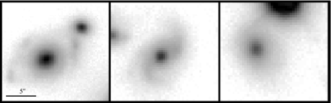
Figure 5.5: R–band image of the four galaxies discussed in the text, with North at top and East to left. Scale is indicated in the left panel.

For the eight red E galaxies having Sersic index less than 2 we suggest that they are a population of disk galaxies. van den Berg, Pierce & Tully (1990), classifying 182 galaxies in the Virgo cluster, have shown the existence of “anemic” spiral galaxies, i.e. spiral galaxies deficient in neutral hydrogen. They have shown that these observations may be accounted for by assuming that gas has been stripped from the outer parts of these objects. Following van den Berg 1991 we recognize these galaxies as Ab-spirals and exclude them from the sample of ellipticals.

HDS_red galaxies have all Sersic indices greater than 3, so they seem to be early-type galaxies.

5.6 Distribution of ages

In order to follow the evolution of galaxies belonging to different spectral classes, we compare the strengths of various spectral indices in the observed galaxy spectra to stellar population models with different star formation rates and metallicities.

Bruzual & Charlot (2003) defined those indices that are most suitable in their models to investigate galaxy populations. They suggested two sets of spectral indices that should be fitted simultaneously in order to break the age-metallicity degeneracy: one of them being primary sensitive to the star formation history (D_n(4000), H_β, H_γA and H_δA) and the other primary sensitive to metallicity ([MgFe]^′,[Mg₁Fe] and [Mg₂Fe]). The latter indices, in fact, are sensitive to metallicity but do not depend sensitively on changes in alpha-element to iron abundance ratios (see Thomas et al. 2003 and Bruzual & Charlot 2003 for details).

For these reasons we use models with different star formation histories in order to fit simultaneously the observed strength of D_n(4000), H_δA, H_γA, H_β, [MgFe]^′, [Mg₁Fe], and [Mg₂Fe].

Figure 5.6: Equivalent width of H_δ versus the break at 4000 Å  for galaxies of different spectral types and GISSEL03 models. Filled and open circles, filled and open triangles, and crosses denote ELG, Ab–spiral, HDS_blue, HDS_red and E galaxies, respectively. The left panel shows models with Z=0.4Z_⊙, central and right panels 1Z_⊙ and 2.5Z_⊙, respectively. In each panel it is plotted a model with exponential declining SFR with time scale $\tau$=1.0 Gyr lasting 11 Gyr (continuous line), with superimposed a burst at t=9 Gyr, involving 10% (dashed line) or 40% (dotted line) of the total mass, and a model with continuous star formation truncated at t=10 Gyr (dot-dashed line).

E-galaxies (crosses in Fig.5.6) exhibit moderate dispersion in D_n(4000), caused by a combination of age and metallicity effects and little star formation. They are well described by an exponentially declining star formation with time scale $\tau$=1.0 Gyr (Merluzzi et al. 2003 and references therein). Assuming this SFR and metallicities Z=0.4 Z_⊙,Z_⊙,2.5 Z_⊙, the distribution of ages for early-type galaxies, (fig. 5.7), shows that the age of the bulk of ellipticals in ABCG 209 is greater than $\sim$ 7 Gyr and that there is a tail toward younger ages up to $\sim$ 4 Gry. This translates into a formation epoch z${}_{f}\mathrel{\hbox{\hbox to0.0pt{\hbox{\lower 4.0pt\hbox{$\sim$}}\hss}\hbox{$>$}}}$ 1.6 for the majority of ellipticals and z${}_{f}\mathrel{\hbox{\hbox to0.0pt{\hbox{\lower 4.0pt\hbox{$\sim$}}\hss}\hbox{$>$}}}$ 0.7 for the younger population. The KMM algorithm (cf. Ashman et al. 1994 and refs. therein) suggests that a mixture of two Gaussians (with $\mathrm{n_{1}=19}$, and $\mathrm{n_{2}=55}$ members) is a better description of this age distribution (although only at $\sim 90\%$ c.l.). In this case, the mean ages of the two distributions are $\mathrm{t_{1}=5.8\pm 0.8}$ Gyr, and $\mathrm{t_{2}=9.2\pm 1.2}$ Gyr respectively. Thus, 74.3% of early-type galaxies seem to be coeval and to be formed early during the initial collapse of the cluster, at z${}_{f}\mathrel{\hbox{\hbox to0.0pt{\hbox{\lower 4.0pt\hbox{$\sim$}}\hss}\hbox{$>$}}}$ 3.5. The remaining 25.7% is constituted by a younger galaxy population, that could be formed later (z${}_{f}\mathrel{\hbox{\hbox to0.0pt{\hbox{\lower 4.0pt\hbox{$\sim$}}\hss}\hbox{$>$}}}$ 1.2) or could have experienced an enhancement in the star formation rate $\sim$ 8.5 Gyr ago. This is in remarkable agreement with the trend with redshift of the total stellar mass in the cluster galaxies, derived from the colour-magnitude relation by Merluzzi et al. 2003 (see their Fig. 10).

As shown in Fig. 5.6 (filled circles), ELG galaxies can be fitted either by a model with truncated star formation history and by a model with a burst involving the 40% of the total mass (Fig. 5.6), whereas the two HDS_blue galaxies, for which we have the measurement of both D_n(4000) and [H_δ], seem to be reproduced only by a model with a short starburst. The starburst is assumed to begin at t=9 Gyr lasting for 0.1 Gyr. An equivalent width of H_δ greater than 5 Å  implies that a starburst occurred in the galaxy before star formation was quenched, otherwise quiescent star formation activity would produce a spectrum with weaker Balmer lines (e.g., Couch & Sharples 1987; Poggianti & Barbaro 1996), as showed also by the comparison of the two models (dotted and dot- dashed lines) in Fig. 5.6. HDS_blue galaxies have EWs stronger than 5 Å, and thus must be post-starburst galaxies. The strength of the lines and the colour of these galaxies indicate an interruption of the star formation within the last 0.5 Gyr, with a strong starburst preceding the quenching of star formation (see also Poggianti et al. 1999; Poggianti & Barbaro 1996).

In contrast, the typical time elapsed since the last star formation in the HDS_red will be in the range 1-2 Gyr, since this population exhibits weaker H_δ equivalent widths. However, the observed [H_δ] values for HDS_red tend to be larger than those predicted by both starburst and truncated star formation models, except from one galaxy that is well reproduced by a burst model (observed $\sim$ 1 Gyr after the burst). This problem was pointed out by several authors (e.g. Couch & Sharples 1987, Morris et al. 1998, Poggianti & Barbaro 1996, Balogh et al. 1999) and will persist if photometric colours are considered instead of D_n(4000).

Models with IMFs biased toward massive stars are able to reproduce better these data. However, the stellar population resulting from such a burst is very short lived ($\sim$ 300 Myr), thus it is unlikely that many of these red galaxies are undergoing such bursts. Stronger [H_δ] may also be produced by temporal variations in the internal reddening in truncated or burst models. Balogh et al. (1999) have shown that by reddening the model it is possible to recover the observed data. This supports the idea that dust obscuration may play an important role in the appearance of these spectra. Recently, in fact, Shioya, Bekki & Couch (2004) demonstrates that the reddest HDS galaxies can only be explained by truncated or starburst models with very heavy dust extinction ($A_{V}>$ 0.5 mag).

Figure 5.7: Distribution of best-fitted ages of E galaxies (continuous line), by using a model with exponential declining SFR with time scale $\tau$=1.0 Gyr. Errors on ages are obtained performing 1000 simulations accounting for equivalent width measurement errors.

5.7 Dynamical scenario

The analysis of the velocity distribution for all member galaxies of ABCG 209 (Mercurio et al. 2003a) shows the existence of a peak at $<z>=0.2090\pm 0.0004$ with a line–of–sight velocity dispersion $\sigma_{v}=1394^{+88}_{-99}$ km s^-1.

In order to check for possible variations of $<z>$ and $\sigma_{v}$ for different spectral types we analysed separately ELG, HDS_blue, Ab-spirals, HDS_red, and E galaxies. All galaxy populations show consistent mean redshift suggesting that they are really cluster populations and not merely foreground or background objects. On the other hand, the velocity dispersions of different classes show significant differences (see Table 5.3).

Table 5.3: Redshifts and velocity dispersion of different spectral classes. The biweight estimators (Beers et al. 1990) were used to derive the values

.

$$\begin{array}[]{c c c c }\hline\cr\vskip 3.0pt plus 1.0pt minus 1.0pt\cr\mathrm{Class}&\mathrm{N_{gal}}&\mathrm{Redshift}&\mathrm{\sigma_{v}}\\ \vskip 3.0pt plus 1.0pt minus 1.0pt\cr\hline\cr\vskip 3.0pt plus 1.0pt minus 1.0pt\cr\mathrm{ALL}&112&0.2090\pm 0.0004&1394_{-99}^{+88}\\ \mathrm{E}&74&0.2086\pm 0.0005&1323_{-94}^{+127}\\ \mathrm{HDS_{red}}&7&0.2087\pm 0.0005&339_{-46}^{+91}\\ \mathrm{Ab-spirals}&8&0.2107\pm 0.0017&1295_{-102}^{+340}\\ \mathrm{HDS_{blue}}&5&0.2071\pm 0.0044&2257_{-65}^{+1085}\\ \mathrm{ELG}&7&0.2070\pm 0.0038&2634_{-53}^{+712}\\ \vskip 3.0pt plus 1.0pt minus 1.0pt\cr\hline\cr\end{array}$$

E galaxies define the mean redshift and the velocity dispersion of the cluster. The very low value of the velocity dispersion of HDS_red galaxies indicates that they could constitute a group of galaxies located at the cluster redshift. These post-starburst galaxies could be the remnant of the core of an infalling clump, that have suffered significant ram–pressure stripping in crossing the cluster core, preceded by an instantaneous burst of star formation.

The groups of ELG and HDS_blue galaxies exhibit very high velocity dispersions. Spectral, photometric and structural properties (cfr. Sect 3.5) of these two classes seem to indicate that they are strongly related, as it is also indicated by the slight difference in the velocity dispersion. The high velocity dispersions of these populations of disk-dominated galaxies indicate that they do not constitute a single infalling bound galaxy group but are the results of the growing of the cluster through the accretion of field galaxies. These facts are in agreement with a scenario in which spirals are accreted into the cluster from the field, then star formation is stopped, the galaxies become gas-deficient, and eventually undergo a morphological transformation (Couch et al. 1998). This scenario may also account for the existence of anemic spirals (Ab-spirals in Table 5.3), whose velocity dispersion is fully consistent with those of the cluster.

Figure 5.8 shows the spatial distribution of different spectral classes. Taking into account the SE-NW elongation of the cluster, ELGs (filled circles) seem to be uniformly distributed in the outer parts of the cluster, while blue HDS galaxies (filled triangles) show a preferential location within the cluster. They are concentrated around the centre of the cluster along a direction perpendicular to the cluster elongation. Ab–spirals (open circles) and E galaxies (crosses) are uniformly distributed over the whole cluster plane and red HDS galaxies (open triangles) lie around the centre along the cluster elongation.

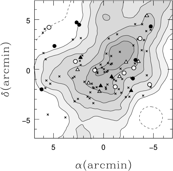
Figure 5.8: Spatial distribution of different spectral classes. Filled and open circles, filled and open triangles, and crosses denote ELG, Ab–spiral, HDS_blue, HDS_red and E galaxies, respectively. The plot is centred on the cluster center. The dashed contour corresponds to the field galaxy number density, while the solid contours correspond respectively to the background subtracted 2, 3.3, 5, 7.5, 10, and 12.5 galaxies arcmin^-2

By using the information about the phase-space distributions, it is possible to find segregations of the various galaxy populations. Biviano et al. (2002) searched for segregation by comparing (R,v)-distributions in the clusters of the ESO Nearby Abell Cluster Survey, using the combined evidence from projected positions and relative velocities (they may not be independent). They also stressed the importance of the estimate of the projected clustercentric distance R, in order to make the comparison as unbiased as possible.

The spatial distribution of galaxies in ABCG 209 shows a complex structure, characterised by an elongation in the SE-NW direction (see Mercurio et al. 2003a). To measure the effect of the cluster environment on the galaxy population, their spectral properties should be measured against the parameter most related to the cluster structure, which is the local galaxy number surface density rather than cluster-centric radius.

The local surface density (LD) of galaxies was determined across the CFHT images by Haines et al. (2004). We performed the comparison of (LD,v)-distributions by means the two–dimensional Kolmogorov–Smirnov test (hereafter 2DKS–test; Press et al. 1992). The 2DKS test is relatively conservative: if it indicates that two distributions have a high probability of not being drawn from the same parent population, other tests (e.g. Rank-Sum tests or Sign Tests) indicate the same thing, while the contrary is not always true. Moreover, the 2DKS test turns out to be reliable with relatively small samples (e.g. Biviano et al. 2002).

According to the 2DKS–test, we find significant evidence for segregation of ELGs with respect to both Es (99.5%) and HDS_blue galaxies (97.6%), where ELGs lie in regions with lower density than E and HDS_blue galaxies. Moreover the distributions of HDS_blue and HDS_red galaxies differ at 90.7% c.l. and HDS_blue and Ab-spirals at 92.0%. These results show the effects of the cluster environment on the spectral properties of their constituents and support the scenario in which ELGs are accreted into the cluster from the field.

5.8 Summary and Discussion

In order to investigate the nature of the galaxy population in ABCG 209, we have performed a detailed study of the photometric and spectroscopic properties of luminous member galaxies (R $\mathrel{\hbox{\hbox to0.0pt{\hbox{\lower 4.0pt\hbox{$\sim$}}\hss}\hbox{$<$}}}$ 20.0). The primary goal of this analysis was to study the relation between cluster dynamics and evolution of stellar populations, and the effects of cluster environment on the properties of galaxies.

ABCG 209 is undergoing strong dynamical evolution with the merging of at least two clumps along the SE-NW direction, as indicated by i) the presence of a velocity gradient along a SE-NW axis, ii) the elongation of X-ray contour levels in Chandra images, and iii) the presence of substructures manifest both in the detection of two peaks separated by 50 arcsec in the X-ray flux and in the analysis of the velocity distribution, that showed three sub-clumps (Mercurio et al. 2003a). Moreover, the young dynamical state of the cluster is indicated by the possible presence of a radio halo (Giovannini, Tordi & Feretti 1999), which has been suggested to be the result of a recent cluster merger, through the acceleration of relativistic particles by the merger shocks (Feretti 2002).

The analysis of the spectroscopic and photometric properties of 102 cluster members has shown the presence of five different types of galaxies: i) passive evolving galaxies (E), which exhibit red colours and no emission lines, ii) emission line galaxies (ELG), which are blue and have prominent emission lines, iii-iv) strong H_δ galaxies, that are characterized by the presence of strong H_δ absorption lines and can be divided into blue (HDS_blue) and red (HDS_red) galaxies, according to the index D_n(4000) and to the B-R colours; v) anemic spirals (Ab-spirals), that have the same spectral properties of passive evolving galaxies, but are disk-dominated systems.

E galaxies represent $\sim$ 74% of the cluster population, and lie mainly in high density regions. Their age distribution is characterized by the presence of an “old population” formed early during the initial collapse of the cluster at ages greater than 7 Gyr, and another one, younger, that could be formed later or could have experienced an enhancement in the star formation rate.

ELGs lie in low density regions and have high line–of–sight velocity dispersion. Both the spatial position and the velocity dispersion suggest that this is a population of galaxies that has recently fallen into the cluster. This infall has induced a truncation of the star formation with, possibly, an associated short starburst.

These results are understandable in terms of cosmological models of structure formation, in which galaxies form earliest in the highest-density regions corresponding to the cores of rich clusters. Not only do the galaxies form earliest here, but the bulk of their star formation is complete by $z\sim 1$, at which point the cluster core is filled by shock-heated virialised gas which does not easily cool or collapse, suppressing the further formation of stars and galaxies (Blanton et al. 1999; 2000). Diaferio et al. (2001) shows that as mixing of the galaxy population is incomplete during cluster assembly, the positions of galaxies within the cluster are correlated with the epoch at which they were accreted. Hence galaxies in the cluster periphery are accreted later, and so have their star formation suppressed later, resulting in younger mean stellar populations. It should be considered however that this is a small-scale affect, and that this result in fact confirms that the red sequence galaxy population is remarkably homogeneous across all environments.

A similar scenario is suggested also by the velocity dispersion and the spectral properties of HDS_blue galaxies, which, however, are found to be aligned in a direction perpendicular to the cluster elongation, that coincides with the elongation of the X-ray contour levels in the Chandra images (see Fig. 14 in Mercurio et al. 2003a). As already pointed out by Poggianti et al. (2004) analysing the position of the strongest k+a galaxies (having [H_δ] $>$ 5 Å) in Coma, the correlation between the location of the post-starburst galaxies and the substructures in the intracluster medium strongly suggest that the truncation of the star formation activity in these galaxies, and possibly the previous starburst, could be the result of an interaction with the hot intracluster medium. Thus, the origin of HDS_blue could be a cluster related and, in particular, an ICM-related phenomenon, closely connected with the dynamical state of the cluster (see Poggianti et al. 2004).

HDS_red galaxies are distributed along the elongation of the cluster, mainly in intermediate density regions and have a low velocity dispersion. According to the evolution models, the presence of strong H_δ absorption line in their spectra indicates that these galaxies have experienced a short starburst of star formation in the past few Gyr. In the starburst model [H_δ] and D_n(4000) declines on a timescale of $\sim$ 2 Gyr after the burst has ceased, regardless of their SFR before the burst. This implies that, in the galaxies we observe, the burst has occurred no more than 4.5 Gyr ago.

As also indicated by the low value of the velocity dispersion, HDS_red galaxies could be the remnant of the core of an infalling clump of galaxies, that have experienced a merger with the main cluster. This merger may have induced a time–dependent tidal gravitational field that stimulated non–axisymmetric perturbations in the galaxies, driving effective transfer of gas to the central galactic region and, finally, triggering a secondary starburst in the central part of these galaxies (Bekki 1999). The second peak of the X-ray distribution could be related to the presence of this small galaxy group.

Considering that the mass is proportional to the cube of the measured velocity dispersion (see eq. (4) and (11) of Girardi et al. 1998), the ratio between the mass of the cluster as constituted only by E galaxies and the group of HDS_red galaxies is $\sim$ 0.017. Taffoni et al. (2003) studied the evolution of dark matter satellites orbiting inside more massive haloes, by using semi-analytical tools coupled with high-resolution N-body simulations. They explored the interplay between dynamic friction and tidal mass loss/evaporation in determining the final fate of the satellite, showing that, for satellites of intermediate mass (0.01 M${}_{\mathrm{h}}<$ M${}_{\mathrm{s,0}}<$ 0.1 M_h, where M_s,0 is the initial mass of the satellite and M_h is the mass of the main halo), the dynamical friction is strong and drives the satellite toward the centre of the main halo, with significant mass loss. The final fate depends on the concentration of the satellite, relative to that of the main halo. Low–concentration satellites are disrupted, while high–concentration satellites survive, with a final mass that depends on the decay time.

Although both HDS_blue and HDS_red are characterized by the presence of strong Balmer lines, their colours and structural parameters show that they are two different galaxy populations. Deriving the Sersic index, we found that HDS_blue galaxies are disk-dominated galaxies while HDS_red are spheroids. On the contrary, Poggianti et al. (2004) found that, with the exception of two blue k+a galaxies compatible with a de Vaucouleurs’ profile, all the other blue and red k+a galaxies in the Coma cluster have exponential or steeper profiles. This apparent contradiction may be overcome by considering the time for a HDS_blue galaxy to become red due to the damping of star formation is shorter than the difference in look-back time between ABCG 209 and Coma. It is thus conceivable that the HDS_blue galaxies we observe at z$\sim$0.21 will turn into HDS_red galaxies observed Coma.

All the presented results support an evolutionary scenario in which ABCG 209 is characterized by the presence of two components: an old galaxy population, formed very early (z${}_{f}\mathrel{\hbox{\hbox to0.0pt{\hbox{\lower 4.0pt\hbox{$\sim$}}\hss}\hbox{$>$}}}$ 3.5) and a younger population of infalling galaxies. Moreover, this cluster may have experienced, 3.5-4.5 Gyr ago, a merging with an infalling galaxy group. The merger of the cluster with the infalling group could have also powered the observed radio halo. In fact, merger activity and high ICM temperature may be responsible for producing a radio halo (Liang et al. 2000), because merging can provide enough energy to accelerate the electrons to relativistic energies, give rising to non-thermal emission. After the shock disappeared, radio halos may be maintained in situ by electron acceleration in the residual turbulence.

Appendix A

The equivalent width is defined by:

$$\mathrm{EW}=\sum^{N}_{i=1}\frac{\mathrm{F_{Ci}}-\mathrm{F_{i}}}{\mathrm{F_{Ci}}}\Delta\lambda\ ,$$ (5.1)

where F_i is the flux in the pixel $i$, $N$ is the number of pixels in the integration range, $\Delta\lambda$ is the dispersion in Å/pixel and F_Ci is the straight line fitted to the blue and the red pseudo–continuum intervals, evaluated in the pixel $i$ (pixels with values more than 3$\sigma$ away from the continuum level were rejected).

An index measured in magnitudes is:

$$\mathrm{Mag}=-2.5\mathrm{log}\left[1-\frac{\mathrm{EW}}{\mathrm{(\lambda_{2}-\lambda_{1})}}\right]\ ,$$ (5.2)

where $\lambda_{1}$ and $\lambda_{2}$ are the wavelength limits of the feature bandpass.

The errors of the equivalent width measurement are estimated from the following relation (Czoske et al. 2001):

$$\sigma^{2}_{EW}=\left(\frac{\mathrm{S}}{\mathrm{N}}\right)^{-2}\left[(N\Delta\lambda-EW)\Delta\lambda+\frac{(N\Delta\lambda-EW)^{2}}{N_{1}+N_{2}}\right]\ ,$$ (5.3)

where S/N is the signal–to–noise ratio evaluated in the feature bandpass.

The local S/N for each galaxy is obtained by dividing the galaxy spectrum by its associated noise spectrum, as determined by adding in quadrature the Poisson noise (obtained through the IRAF task APALL) and the read-out noise of EMMI. The result is then fitted to remove residual features, and averaged over the wavelength range of the spectral feature to obtain the S/N ratio.

The catalogue of spectroscopic measurements is presented in Table  5.4.

Table 5.4: Spectroscopic data. Running number for galaxies in the presented sample (see also Table 5.1), ID (Col. 1); strength of the 4000 Å  break (Col. 2); Cols. 3-15: equivalent widths. A value of ’0.0’ for the equivalent width for an emission-line indicates that no emission is observed, whereas ’….’ indicates that the equivalent width could not be measured as the line does not lie within the available wavelength range. The spectral classification adopted in the present paper is listed in the last column. ELG: emission line galaxies; HDS_blue: H_δ strong galaxies with blue colour; HDS_red: H_δ strong galaxies with red colour; E: passive evolving galaxies; Ab-spirals: passive evolving disk-dominated galaxies (n${}_{\mathrm{Sersic}}\leq$ 2). Galaxy 62 is referred to as AGN because it shows the signature of a galactic active nucleus and is excluded from the analysis.

$$\begin{array}[]{c c c c c c c c c c c c c c c c }\hline\cr\vskip 3.0pt plus 1.0pt minus 1.0pt\cr\hline\cr\vskip 3.0pt plus 1.0pt minus 1.0pt\cr\mathrm{ID}&\mathrm{D_{n}(4000)}&\mathrm{[OII]}&\mathrm{H_{\delta A}}&\mathrm{H_{\gamma A}}&\mathrm{Fe4531}&\mathrm{H_{\beta}}&\mathrm{[OIII]}&\mathrm{Fe5015}&\mathrm{Mg_{1}}&\mathrm{Mg_{2}}&\mathrm{Mg}b&\mathrm{Fe5270}&\mathrm{Fe5335}&\mathrm{H_{\alpha}}&\mathrm{Spectral}\\ &\AA&\AA&\AA&\AA&\AA&\AA&\AA&\AA&\mathrm{mag}&\mathrm{mag}&\AA&\AA&\AA&\AA&\mathrm{class}\\ \hline\cr\vskip 3.0pt plus 1.0pt minus 1.0pt\cr 1&1.14\pm 0.06&-10.1\pm 1.2&7.1\pm 0.8&0.3\pm 0.8&4.7\pm 1.0&-0.5\pm 0.6&-0.3\pm 0.4&5.2\pm 1.2&0.07\pm 0.01&0.21\pm 0.02&3.4\pm 0.5&2.7\pm 0.6&2.0\pm 0.7&-10.8\pm 0.9&\mathrm{ELG}\\ 2&1.73\pm 0.03&0.0&-1.0\pm 0.8&-4.2\pm 0.7&4.3\pm 0.7&1.6\pm 0.5&0.0&6.1\pm 0.9&0.16\pm 0.01&0.30\pm 0.01&3.6\pm 0.4&3.6\pm 0.5&2.7\pm 0.6&2.5\pm 0.4&\mathrm{E}\\ 3&1.93\pm 0.05&0.0&1.0\pm 1.2&-2.8\pm 1.1&2.9\pm 1.1&2.5\pm 0.7&0.0&7.4\pm 1.3&0.15\pm 0.02&0.33\pm 0.02&5.6\pm 0.6&5.4\pm 0.7&2.2\pm 0.9&2.7\pm 0.6&\mathrm{E}\\ 4&....&....&-4.0\pm 2.2&1.4\pm 1.8&2.4\pm 2.1&4.2\pm 1.3&0.0&11.3\pm 2.5&0.12\pm 0.03&0.18\pm 0.04&3.9\pm 1.3&5.5\pm 1.4&3.4\pm 1.6&5.5\pm 1.2&\mathrm{E}\\ 5&1.72\pm 0.09&....&-6.8\pm 2.4&-1.8\pm 1.6&-0.4\pm 1.8&5.3\pm 1.0&0.0&5.4\pm 2.1&0.10\pm 0.02&0.27\pm 0.03&1.3\pm 1.0&5.9\pm 1.0&2.0\pm 1.3&-4.2\pm 1.1&\mathrm{Ab-spiral}\\ 6&1.89\pm 0.07&0.0&3.5\pm 0.4&-9.0\pm 0.5&2.6\pm 0.5&2.8\pm 0.3&0.0&10.6\pm 0.7&0.19\pm 0.01&0.44\pm 0.01&6.9\pm 0.3&6.4\pm 0.4&5.8\pm 0.5&3.6\pm 0.4&\mathrm{HDS_{red}}\\ 7&1.70\pm 0.03&0.0&-1.3\pm 0.7&-3.0\pm 0.6&4.1\pm 0.7&1.9\pm 0.4&0.0&5.1\pm 0.8&0.16\pm 0.01&0.34\pm 0.01&4.3\pm 0.4&3.1\pm 0.4&2.2\pm 0.5&0.3\pm 0.4&\mathrm{E}\\ 8&1.73\pm 0.05&0.0&1.0\pm 1.2&-3.9\pm 1.0&4.7\pm 1.0&1.3\pm 0.6&0.0&7.5\pm 1.2&0.19\pm 0.02&0.36\pm 0.02&5.2\pm 0.6&3.9\pm 0.7&2.3\pm 0.8&0.4\pm 0.6&\mathrm{E}\\ 9&....&....&-1.6\pm 1.6&-0.3\pm 1.3&4.8\pm 1.4&1.1\pm 0.9&0.0&6.0\pm 1.7&0.17\pm 0.02&0.34\pm 0.03&4.1\pm 0.8&4.4\pm 0.9&6.2\pm 1.0&0.4\pm 0.8&\mathrm{E}\\ 10&1.66\pm 0.06&....&-1.8\pm 1.7&-3.5\pm 1.4&4.2\pm 1.4&2.0\pm 1.0&0.0&7.0\pm 1.9&0.15\pm 0.02&0.31\pm 0.03&4.9\pm 0.8&3.1\pm 0.9&4.3\pm 1.1&4.6\pm 0.7&\mathrm{E}\\ 11&1.77\pm 0.04&0.0&-1.3\pm 0.9&-4.6\pm 0.8&4.4\pm 0.9&2.8\pm 0.5&0.0&5.4\pm 1.1&0.17\pm 0.01&0.32\pm 0.02&5.1\pm 0.5&3.1\pm 0.6&1.9\pm 0.6&1.8\pm 0.5&\mathrm{E}\\ 12&....&....&-2.7\pm 1.7&-8.4\pm 1.5&4.4\pm 1.6&4.0\pm 1.0&0.0&7.5\pm 2.0&0.24\pm 0.03&0.31\pm 0.03&4.0\pm 0.9&8.1\pm 1.0&2.8\pm 1.2&1.7\pm 1.0&\mathrm{E}\\ 13&....&....&2.8\pm 1.8&-2.8\pm 1.6&4.4\pm 1.7&1.0\pm 1.1&0.0&8.3\pm 2.0&0.14\pm 0.03&0.27\pm 0.03&2.8\pm 1.0&7.1\pm 1.0&4.7\pm 1.2&1.4\pm 0.9&\mathrm{E}\\ 14&2.08\pm 0.05&0.0&-0.7\pm 1.3&-2.8\pm 1.1&6.2\pm 1.2&3.2\pm 0.8&0.0&7.1\pm 1.6&0.17\pm 0.02&0.33\pm 0.02&4.2\pm 0.7&3.3\pm 0.8&1.9\pm 1.0&4.4\pm 0.6&\mathrm{Ab-spiral}\\ 15&....&....&3.9\pm 1.8&-2.1\pm 1.7&5.7\pm 2.0&5.8\pm 1.2&0.0&10.2\pm 2.3&0.11\pm 0.03&0.25\pm 0.04&3.8\pm 1.2&3.9\pm 1.3&6.0\pm 1.5&4.1\pm 1.2&\mathrm{HDS_{red}}\\ 16&1.80\pm 0.05&....&0.8\pm 1.7&-2.4\pm 1.4&5.8\pm 1.4&2.1\pm 0.9&0.0&5.9\pm 1.8&0.14\pm 0.02&0.27\pm 0.03&6.3\pm 0.8&3.3\pm 0.9&3.8\pm 1.1&1.7\pm 0.8&\mathrm{E}\\ 17&1.31\pm 0.03&....&9.5\pm 0.7&8.0\pm 0.7&3.0\pm 1.1&4.8\pm 0.6&-1.0\pm 0.5&3.6\pm 1.4&0.07\pm 0.02&0.15\pm 0.02&3.5\pm 0.7&4.0\pm 0.7&3.1\pm 0.9&-7.5\pm 0.9&\mathrm{ELG}\\ 18&....&....&-1.1\pm 1.7&-3.8\pm 1.5&5.8\pm 1.5&2.5\pm 1.0&0.0&9.0\pm 1.9&0.16\pm 0.02&0.34\pm 0.03&6.9\pm 0.9&4.5\pm 1.0&1.2\pm 1.3&2.5\pm 1.0&\mathrm{E}\\ 19&1.98\pm 0.05&....&-0.6\pm 1.0&1.5\pm 0.8&6.1\pm 0.8&2.4\pm 0.5&0.0&4.9\pm 1.0&0.15\pm 0.01&0.26\pm 0.01&5.0\pm 0.4&3.0\pm 0.5&7.4\pm 0.6&0.5\pm 0.4&\mathrm{E}\\ 20&1.66\pm 0.04&0.0&1.4\pm 3.0&-8.3\pm 2.7&4.5\pm 2.9&6.6\pm 1.7&0.0&7.2\pm 3.4&0.13\pm 0.04&0.30\pm 0.05&2.7\pm 1.7&2.7\pm 1.8&2.2\pm 2.1&1.7\pm 1.6&\mathrm{Ab-spiral}\\ 21&1.82\pm 0.04&0.0&-1.2\pm 1.1&-3.1\pm 0.9&4.9\pm 1.1&2.5\pm 0.7&0.0&7.5\pm 1.2&0.13\pm 0.02&0.29\pm 0.02&5.0\pm 0.6&3.4\pm 0.6&2.8\pm 0.8&3.4\pm 0.5&\mathrm{E}\\ 22&1.17\pm 0.05&....&4.6\pm 2.1&1.7\pm 1.0&8.7\pm 1.2&-3.0\pm 0.9&-2.5\pm 0.5&7.1\pm 1.5&0.04\pm 0.02&0.10\pm 0.02&4.7\pm 0.6&2.5\pm 0.8&7.2\pm 0.7&-5.6\pm 0.7&\mathrm{ELG}\\ 23&1.67\pm 0.04&0.0&-2.1\pm 0.9&-4.0\pm 0.8&4.9\pm 0.9&2.1\pm 0.6&0.0&6.0\pm 1.1&0.13\pm 0.01&0.26\pm 0.02&4.6\pm 0.5&4.9\pm 0.6&3.3\pm 0.7&2.7\pm 0.5&\mathrm{E}\\ \vskip 3.0pt plus 1.0pt minus 1.0pt\cr\hline\cr\end{array}$$

Table 5.4: Continued.

$$\begin{array}[]{c c c c c c c c c c c c c c c c}\hline\cr\vskip 3.0pt plus 1.0pt minus 1.0pt\cr\hline\cr\vskip 3.0pt plus 1.0pt minus 1.0pt\cr\mathrm{ID}&\mathrm{D_{n}(4000)}&\mathrm{[OII]}&\mathrm{H_{\delta A}}&\mathrm{H_{\gamma A}}&\mathrm{Fe4531}&\mathrm{H_{\beta}}&\mathrm{[OIII]}&\mathrm{Fe5015}&\mathrm{Mg_{1}}&\mathrm{Mg_{2}}&\mathrm{Mg}b&\mathrm{Fe5270}&\mathrm{Fe5335}&\mathrm{H_{\alpha}}&\mathrm{Spectral}\\ &\AA&\AA&\AA&\AA&\AA&\AA&\AA&\AA&\mathrm{mag}&\mathrm{mag}&\AA&\AA&\AA&\AA&\mathrm{class}\\ \hline\cr\vskip 3.0pt plus 1.0pt minus 1.0pt\cr 24&1.38\pm 0.06&....&7.8\pm 1.2&7.7\pm 1.1&4.0\pm 1.5&7.2\pm 0.8&0.0&7.4\pm 1.8&-.02\pm 0.02&0.11\pm 0.03&3.8\pm 0.9&4.9\pm 1.1&-0.6\pm 1.5&0.7\pm 1.1&\mathrm{HDS_{blue}}\\ 25&1.84\pm 0.11&0.0&-5.2\pm 1.9&-5.5\pm 1.3&3.7\pm 1.3&5.3\pm 0.7&0.0&6.7\pm 1.4&0.15\pm 0.02&0.30\pm 0.02&4.8\pm 0.6&3.5\pm 0.7&3.3\pm 0.9&....&\mathrm{E}\\ 26&1.70\pm 0.03&....&-1.6\pm 1.0&-2.8\pm 0.8&5.2\pm 1.0&2.5\pm 0.6&0.0&6.0\pm 1.1&0.11\pm 0.01&0.27\pm 0.02&4.6\pm 0.6&2.5\pm 0.6&4.2\pm 0.7&2.9\pm 0.5&\mathrm{E}\\ 27&....&....&4.6\pm 2.2&-7.3\pm 2.2&11.8\pm 1.8&-0.3\pm 1.3&0.0&7.6\pm 2.5&0.18\pm 0.03&0.38\pm 0.04&7.6\pm 1.1&5.9\pm 1.3&4.9\pm 1.5&7.1\pm 1.0&\mathrm{HDS_{red}}\\ 28&1.67\pm 0.04&0.0&-2.0\pm 1.3&-2.8\pm 1.1&4.9\pm 1.1&5.1\pm 0.7&0.0&7.4\pm 1.4&0.13\pm 0.02&0.30\pm 0.02&4.8\pm 0.7&2.8\pm 0.7&2.8\pm 0.9&....&\mathrm{E}\\ 29&1.58\pm 0.06&0.0&2.6\pm 1.4&3.9\pm 1.1&5.6\pm 1.2&5.8\pm 0.7&0.0&5.4\pm 1.5&0.04\pm 0.02&0.16\pm 0.02&3.4\pm 0.7&4.9\pm 0.8&3.2\pm 0.9&3.6\pm 0.7&\mathrm{Ab-spiral}\\ 30&1.66\pm 0.03&0.0&-0.8\pm 0.6&-4.1\pm 0.5&4.3\pm 0.6&2.0\pm 0.4&0.0&5.2\pm 0.7&0.12\pm 0.01&0.29\pm 0.01&4.9\pm 0.3&3.1\pm 0.4&2.1\pm 0.5&-0.3\pm 0.4&\mathrm{E}\\ 31&1.87\pm 0.08&0.0&-1.5\pm 2.2&-1.5\pm 1.6&-1.9\pm 1.8&4.1\pm 0.9&0.0&6.9\pm 1.7&0.15\pm 0.02&0.30\pm 0.03&6.2\pm 0.8&5.5\pm 0.9&2.5\pm 1.0&1.2\pm 0.7&\mathrm{E}\\ 32&1.83\pm 0.04&0.0&0.6\pm 0.7&-4.5\pm 0.7&4.0\pm 0.7&3.0\pm 0.5&0.0&7.6\pm 0.9&0.15\pm 0.01&0.29\pm 0.01&4.2\pm 0.4&2.8\pm 0.5&1.2\pm 0.6&3.2\pm 0.4&\mathrm{E}\\ 33&1.83\pm 0.06&0.0&0.8\pm 0.8&-3.6\pm 0.8&3.4\pm 0.8&2.7\pm 0.5&0.0&5.6\pm 1.0&0.21\pm 0.01&0.39\pm 0.02&6.4\pm 0.5&3.5\pm 0.5&3.0\pm 0.6&2.3\pm 0.5&\mathrm{E}\\ 34&1.58\pm 0.10&0.0&4.5\pm 1.5&-3.7\pm 1.3&8.5\pm 1.3&4.9\pm 0.7&0.0&7.0\pm 1.5&0.09\pm 0.02&0.32\pm 0.02&6.4\pm 0.7&5.1\pm 0.8&0.9\pm 1.0&2.7\pm 0.6&\mathrm{HDS_{red}}\\ 35&1.73\pm 0.04&0.0&-2.1\pm 0.9&-3.5\pm 0.8&5.6\pm 0.8&3.6\pm 0.5&0.0&8.3\pm 1.0&0.13\pm 0.01&0.40\pm 0.02&7.1\pm 0.4&4.4\pm 0.5&4.7\pm 0.5&....&\mathrm{E}\\ 36&1.65\pm 0.06&....&0.2\pm 2.3&-3.5\pm 1.7&2.7\pm 1.9&2.5\pm 1.1&0.0&8.8\pm 2.1&0.14\pm 0.03&0.32\pm 0.03&4.9\pm 1.0&12.1\pm 1.0&3.8\pm 1.3&4.9\pm 0.9&\mathrm{E}\\ 37&1.97\pm 0.05&0.0&-1.2\pm 0.9&-5.1\pm 0.8&4.8\pm 0.7&1.4\pm 0.5&0.0&4.0\pm 1.0&0.18\pm 0.01&0.43\pm 0.02&6.5\pm 0.4&2.8\pm 0.5&2.4\pm 0.6&2.4\pm 0.5&\mathrm{E}\\ 38&1.95\pm 0.07&0.0&-4.0\pm 1.3&-3.3\pm 1.0&6.7\pm 0.9&3.2\pm 0.5&0.0&4.5\pm 1.0&0.21\pm 0.01&0.39\pm 0.02&6.3\pm 0.5&4.4\pm 0.5&2.9\pm 0.7&-0.4\pm 0.4&\mathrm{E}\\ 39&1.79\pm 0.04&0.0&-1.4\pm 0.8&-4.0\pm 0.7&4.7\pm 0.8&3.7\pm 0.5&0.0&7.1\pm 0.9&0.14\pm 0.01&0.36\pm 0.01&6.4\pm 0.4&3.5\pm 0.5&3.1\pm 0.6&2.3\pm 0.5&\mathrm{Ab-spiral}\\ 40&1.56\pm 0.10&....&-3.6\pm 2.3&1.8\pm 1.6&3.7\pm 1.9&2.0\pm 1.1&0.0&8.8\pm 2.1&0.04\pm 0.03&0.20\pm 0.03&4.1\pm 0.9&4.0\pm 1.1&5.3\pm 1.3&2.1\pm 0.9&\mathrm{E}\\ 41&1.85\pm 0.07&....&2.3\pm 1.8&-2.2\pm 1.4&9.0\pm 1.3&2.2\pm 0.9&0.0&10.4\pm 1.6&0.14\pm 0.02&0.29\pm 0.03&4.3\pm 0.7&2.4\pm 0.9&3.4\pm 1.0&4.3\pm 0.6&\mathrm{E}\\ 42&1.56\pm 0.10&....&-0.8\pm 2.2&3.9\pm 1.6&0.9\pm 2.0&3.6\pm 1.3&0.0&1.3\pm 2.6&0.12\pm 0.03&0.29\pm 0.04&5.6\pm 1.2&5.4\pm 1.2&2.3\pm 1.5&1.9\pm 1.1&\mathrm{E}\\ 43&1.19\pm 0.03&0.0&9.9\pm 0.3&6.7\pm 0.3&2.4\pm 0.5&7.7\pm 0.3&0.0&4.5\pm 0.6&0.04\pm 0.01&0.13\pm 0.01&1.7\pm 0.3&2.3\pm 0.4&2.5\pm 0.5&1.5\pm 0.4&\mathrm{HDS_{blue}}\\ 44&1.93\pm 0.05&0.0&-2.4\pm 1.4&-2.2\pm 1.1&4.9\pm 1.3&4.2\pm 0.7&0.0&7.1\pm 1.6&0.15\pm 0.02&0.38\pm 0.02&5.5\pm 0.7&3.5\pm 0.8&3.5\pm 0.9&-1.9\pm 0.8&\mathrm{E}\\ 45&1.98\pm 0.08&....&-2.9\pm 1.8&-3.7\pm 1.4&4.7\pm 1.5&3.6\pm 0.8&0.0&3.6\pm 1.7&0.22\pm 0.02&0.28\pm 0.02&7.2\pm 0.7&6.1\pm 0.8&4.2\pm 1.0&2.3\pm 0.8&\mathrm{E}\\ 46&1.83\pm 0.06&....&-2.6\pm 1.2&-4.7\pm 1.0&6.9\pm 1.1&3.2\pm 0.6&0.0&9.0\pm 1.2&0.24\pm 0.02&0.33\pm 0.02&1.5\pm 0.6&2.0\pm 0.7&3.0\pm 0.8&-1.4\pm 0.6&\mathrm{E}\\ 47&1.70\pm 0.04&0.0&-0.5\pm 0.8&-2.8\pm 0.7&5.6\pm 0.8&1.6\pm 0.5&0.0&6.1\pm 1.0&0.17\pm 0.01&0.35\pm 0.02&4.5\pm 0.5&3.9\pm 0.5&3.6\pm 0.6&3.4\pm 0.5&\mathrm{E}\\ 48&1.57\pm 0.08&0.0&-1.3\pm 1.8&-2.1\pm 1.5&4.1\pm 1.5&2.5\pm 0.9&0.0&9.4\pm 1.6&0.19\pm 0.02&0.29\pm 0.03&6.1\pm 0.8&2.1\pm 0.9&2.9\pm 1.0&3.4\pm 0.7&\mathrm{E}\\ 49&1.82\pm 0.03&....&-0.9\pm 0.7&-1.6\pm 0.6&6.0\pm 0.6&2.6\pm 0.4&0.0&6.0\pm 0.7&0.12\pm 0.01&0.30\pm 0.01&4.6\pm 0.3&3.2\pm 0.4&3.2\pm 0.5&....&\mathrm{E}\\ 50&....&....&-1.5\pm 0.7&-5.7\pm 0.6&4.0\pm 0.6&2.4\pm 0.4&0.0&5.8\pm 0.7&0.17\pm 0.01&0.35\pm 0.01&4.3\pm 0.3&3.6\pm 0.4&2.9\pm 0.4&3.7\pm 0.3&\mathrm{E}\\ \vskip 3.0pt plus 1.0pt minus 1.0pt\cr\hline\cr\end{array}$$

Table 5.4: Continued.

$$\begin{array}[]{c c c c c c c c c c c c c c c c c}\hline\cr\vskip 3.0pt plus 1.0pt minus 1.0pt\cr\hline\cr\vskip 3.0pt plus 1.0pt minus 1.0pt\cr\mathrm{ID}&\mathrm{D_{n}(4000)}&\mathrm{[OII]}&\mathrm{H_{\delta A}}&\mathrm{H_{\gamma A}}&\mathrm{Fe4531}&\mathrm{H_{\beta}}&\mathrm{[OIII]}&\mathrm{Fe5015}&\mathrm{Mg_{1}}&\mathrm{Mg_{2}}&\mathrm{Mg}b&\mathrm{Fe5270}&\mathrm{Fe5335}&\mathrm{H_{\alpha}}&\mathrm{Spectral}\\ &\AA&\AA&\AA&\AA&\AA&\AA&\AA&\AA&\mathrm{mag}&\mathrm{mag}&\AA&\AA&\AA&\AA&\mathrm{class}\\ \hline\cr\vskip 3.0pt plus 1.0pt minus 1.0pt\cr 51&1.65\pm 0.04&0.0&-1.0\pm 0.7&-1.1\pm 0.6&3.4\pm 0.7&3.6\pm 0.4&0.0&6.1\pm 0.8&0.12\pm 0.01&0.29\pm 0.01&4.3\pm 0.4&3.9\pm 0.5&2.9\pm 0.6&4.1\pm 0.4&\mathrm{E}\\ 52&1.81\pm 0.04&0.0&-1.8\pm 0.9&-3.3\pm 0.8&3.8\pm 0.8&2.4\pm 0.5&0.0&5.8\pm 1.0&0.17\pm 0.01&0.37\pm 0.02&5.7\pm 0.5&2.5\pm 0.5&2.8\pm 0.6&2.3\pm 0.5&\mathrm{E}\\ 53&1.51\pm 0.09&0.0&2.9\pm 3.3&-5.0\pm 2.3&4.5\pm 2.2&1.2\pm 1.2&0.0&5.4\pm 2.3&0.15\pm 0.03&0.34\pm 0.04&5.0\pm 1.0&2.1\pm 1.2&6.1\pm 1.3&4.1\pm 0.9&\mathrm{E}\\ 54&2.11\pm 0.05&0.0&-1.2\pm 0.9&-2.3\pm 0.8&4.1\pm 0.8&3.4\pm 0.5&0.0&7.8\pm 0.9&0.17\pm 0.01&0.39\pm 0.02&5.7\pm 0.5&4.3\pm 0.5&2.4\pm 0.7&2.3\pm 0.4&\mathrm{E}\\ 55&1.77\pm 0.04&0.0&-2.6\pm 0.6&-6.4\pm 0.6&4.9\pm 0.6&3.7\pm 0.4&0.0&5.0\pm 0.7&0.17\pm 0.01&0.41\pm 0.01&6.5\pm 0.3&2.2\pm 0.4&3.2\pm 0.5&1.4\pm 0.4&\mathrm{E}\\ 56&1.86\pm 0.05&0.0&-2.1\pm 1.0&-4.3\pm 0.8&2.6\pm 0.8&3.3\pm 0.5&0.0&4.9\pm 0.9&0.15\pm 0.01&0.38\pm 0.01&6.4\pm 0.4&2.9\pm 0.5&2.6\pm 0.6&0.7\pm 0.4&\mathrm{E}\\ 57&....&....&4.5\pm 1.3&0.3\pm 1.2&4.0\pm 1.4&1.5\pm 0.8&0.0&4.4\pm 1.6&0.08\pm 0.02&0.18\pm 0.02&3.2\pm 0.8&4.9\pm 0.8&3.3\pm 1.0&0.5\pm 0.7&\mathrm{HDS_{blue}}\\ 58&1.66\pm 0.03&0.0&-1.4\pm 0.8&-5.6\pm 0.7&5.0\pm 0.8&0.6\pm 0.5&0.0&5.5\pm 1.0&0.17\pm 0.01&0.39\pm 0.02&4.6\pm 0.5&3.4\pm 0.5&3.3\pm 0.7&2.5\pm 0.5&\mathrm{E}\\ 59&1.73\pm 0.08&0.0&6.4\pm 1.3&-2.9\pm 1.1&6.4\pm 1.1&-0.4\pm 0.7&0.0&8.9\pm 1.1&0.14\pm 0.01&0.29\pm 0.02&5.9\pm 0.6&3.7\pm 0.6&2.3\pm 0.8&1.9\pm 0.5&\mathrm{HDS_{red}}\\ 60&1.70\pm 0.06&0.0&0.5\pm 1.3&-3.3\pm 1.0&4.8\pm 1.0&3.0\pm 0.6&0.0&6.1\pm 1.2&0.15\pm 0.01&0.39\pm 0.02&7.5\pm 0.5&4.3\pm 0.6&4.0\pm 0.7&1.9\pm 0.5&\mathrm{E}\\ 61&1.69\pm 0.04&0.0&-3.5\pm 2.5&-2.5\pm 2.1&4.8\pm 2.4&2.3\pm 1.5&0.0&7.7\pm 2.7&0.19\pm 0.04&0.34\pm 0.05&5.5\pm 1.3&2.6\pm 1.6&4.4\pm 1.7&2.0\pm 1.2&\mathrm{E}\\ 62&1.09\pm 0.01&-57.6\pm 1.8&4.5\pm 1.1&-3.4\pm 1.2&6.5\pm 1.3&-19.1\pm 1.2&-22.9\pm 0.8&-11.4\pm 1.9&0.06\pm 0.02&0.05\pm 0.02&0.7\pm 0.9&1.2\pm 1.0&0.7\pm 1.1&-123.3\pm 1.6&\mathrm{AGN}\\ 63&....&....&-2.2\pm 1.1&-3.2\pm 1.0&4.4\pm 0.9&2.5\pm 0.5&0.0&5.1\pm 1.1&0.16\pm 0.01&0.37\pm 0.02&5.1\pm 0.5&4.2\pm 0.6&2.8\pm 0.7&1.3\pm 0.5&\mathrm{E}\\ 64&....&....&3.2\pm 1.3&-0.1\pm 1.3&4.4\pm 1.5&0.6\pm 1.1&0.0&4.8\pm 1.9&0.08\pm 0.02&0.20\pm 0.03&2.8\pm 0.9&4.6\pm 1.0&2.4\pm 1.3&-10.6\pm 1.1&\mathrm{HDS_{blue}}\\ 65&1.63\pm 0.04&0.0&-3.2\pm 1.2&-3.5\pm 1.0&6.3\pm 1.1&3.3\pm 0.7&0.0&7.8\pm 1.4&0.15\pm 0.02&0.21\pm 0.02&6.9\pm 0.7&4.5\pm 0.8&0.8\pm 0.9&-1.0\pm 0.8&\mathrm{Ab-spiral}\\ 66&....&....&-1.0\pm 1.6&-2.1\pm 1.3&4.4\pm 1.2&1.8\pm 0.8&0.0&7.0\pm 1.5&0.15\pm 0.02&0.32\pm 0.02&5.3\pm 0.6&3.6\pm 0.8&3.1\pm 0.9&2.1\pm 0.6&\mathrm{E}\\ 67&1.54\pm 0.10&....&1.2\pm 2.5&4.4\pm 1.7&10.5\pm 1.7&4.5\pm 1.1&0.0&-0.7\pm 2.2&0.17\pm 0.03&0.34\pm 0.03&2.9\pm 1.0&2.7\pm 1.1&2.1\pm 1.3&....&\mathrm{E}\\ 68&1.85\pm 0.03&0.0&-2.3\pm 0.5&-4.3\pm 0.5&4.6\pm 0.5&4.2\pm 0.3&0.0&6.5\pm 0.6&0.17\pm 0.01&0.38\pm 0.01&5.8\pm 0.3&3.5\pm 0.3&3.1\pm 0.4&1.5\pm 0.3&\mathrm{E}\\ 69&2.01\pm 0.06&0.0&-1.3\pm 1.3&-5.8\pm 1.1&4.3\pm 1.0&1.4\pm 0.7&0.0&6.5\pm 1.2&0.17\pm 0.01&0.40\pm 0.02&7.7\pm 0.5&4.5\pm 0.6&2.3\pm 0.7&2.5\pm 0.5&\mathrm{E}\\ 70&....&....&1.2\pm 1.7&-3.1\pm 1.4&2.9\pm 1.4&0.0&0.0&5.1\pm 1.7&0.13\pm 0.02&0.23\pm 0.02&3.8\pm 0.7&2.5\pm 0.8&3.7\pm 1.0&1.7\pm 0.5&\mathrm{E}\\ 71&1.98\pm 0.04&0.0&-1.1\pm 0.9&-3.0\pm 0.7&4.6\pm 0.8&3.3\pm 0.5&0.0&5.2\pm 0.9&0.18\pm 0.01&0.36\pm 0.02&5.1\pm 0.4&3.9\pm 0.5&2.2\pm 0.6&....&\mathrm{E}\\ 72&1.82\pm 0.11&....&4.9\pm 2.4&-11.1\pm 2.2&4.4\pm 2.0&5.1\pm 1.2&0.0&2.4\pm 2.3&0.20\pm 0.03&0.22\pm 0.03&5.5\pm 1.0&6.0\pm 1.1&4.3\pm 1.3&3.6\pm 0.9&\mathrm{HDS_{red}}\\ 73&1.87\pm 0.04&0.0&-0.9\pm 0.8&-3.7\pm 0.6&4.2\pm 0.7&3.7\pm 0.4&0.0&8.4\pm 0.9&0.16\pm 0.01&0.39\pm 0.01&6.1\pm 0.4&3.9\pm 0.4&3.3\pm 0.6&....&\mathrm{E}\\ 74&1.71\pm 0.04&0.0&0.1\pm 0.4&-3.6\pm 0.4&4.3\pm 0.5&2.6\pm 0.3&0.0&4.8\pm 0.7&0.14\pm 0.01&0.22\pm 0.01&2.3\pm 0.3&4.9\pm 0.4&3.2\pm 0.5&4.3\pm 0.3&\mathrm{E}\\ 75&1.93\pm 0.07&0.0&3.0\pm 1.3&-5.6\pm 1.4&2.0\pm 1.6&3.3\pm 1.3&0.0&2.6\pm 2.7&0.25\pm 0.04&0.79\pm 0.05&16.7\pm 1.0&-1.7\pm 1.6&0.6\pm 2.0&....&\mathrm{E}\\ 76&1.62\pm 0.04&0.0&-1.8\pm 1.0&-4.0\pm 0.9&2.7\pm 1.1&6.0\pm 0.7&0.0&3.1\pm 1.5&0.23\pm 0.02&0.42\pm 0.02&4.4\pm 0.7&3.1\pm 0.8&5.2\pm 0.9&....&\mathrm{E}\\ 77&1.71\pm 0.05&0.0&-2.7\pm 1.0&-6.1\pm 0.9&5.1\pm 1.0&1.9\pm 0.7&0.0&5.5\pm 1.4&0.20\pm 0.02&0.42\pm 0.02&5.6\pm 0.7&1.4\pm 0.8&2.5\pm 1.0&....&\mathrm{E}\\ \vskip 3.0pt plus 1.0pt minus 1.0pt\cr\hline\cr\end{array}$$

Table 5.4: Continued.

$$\begin{array}[]{c c c c c c c c c c c c c c c c}\hline\cr\vskip 3.0pt plus 1.0pt minus 1.0pt\cr\hline\cr\vskip 3.0pt plus 1.0pt minus 1.0pt\cr\mathrm{ID}&\mathrm{D_{n}(4000)}&\mathrm{[OII]}&\mathrm{H_{\delta A}}&\mathrm{H_{\gamma A}}&\mathrm{Fe4531}&\mathrm{H_{\beta}}&\mathrm{[OIII]}&\mathrm{Fe5015}&\mathrm{Mg_{1}}&\mathrm{Mg_{2}}&\mathrm{Mg}b&\mathrm{Fe5270}&\mathrm{Fe5335}&\mathrm{H_{\alpha}}&\mathrm{Spectral}\\ &&\AA&\AA&\AA&\AA&\AA&\AA&\AA&\AA&\mathrm{mag}&\mathrm{mag}&\AA&\AA&\AA&\mathrm{class}\\ \hline\cr\vskip 3.0pt plus 1.0pt minus 1.0pt\cr 78&....&....&2.3\pm 2.9&0.5\pm 3.1&3.8\pm 3.5&4.5\pm 2.2&0.0&14.5\pm 5.9&0.02\pm 0.08&0.15\pm 0.10&4.8\pm 3.3&11.0\pm 3.2&-6.9\pm 6.1&....&\mathrm{E}\\ 79&....&....&5.1\pm 0.6&5.0\pm 0.5&3.1\pm 0.7&4.5\pm 0.4&0.0&6.6\pm 0.8&0.08\pm 0.01&0.19\pm 0.01&3.2\pm 0.4&3.8\pm 0.5&3.9\pm 0.6&2.5\pm 0.5&\mathrm{HDS_{blue}}\\ 80&....&....&0.3\pm 1.6&-4.7\pm 1.6&5.2\pm 1.8&4.4\pm 1.1&0.0&12.1\pm 2.2&0.10\pm 0.03&0.38\pm 0.04&6.1\pm 1.1&0.6\pm 1.4&5.2\pm 1.4&-3.6\pm 1.4&\mathrm{E}\\ 81&1.31\pm 0.05&-6.1\pm 1.7&5.1\pm 1.3&3.5\pm 1.3&4.8\pm 1.6&1.6\pm 1.1&-0.2\pm 0.8&0.5\pm 2.3&0.07\pm 0.03&0.23\pm 0.04&0.9\pm 1.2&6.0\pm 1.1&3.0\pm 1.4&-4.1\pm 1.3&\mathrm{ELG}\\ 82&....&....&-2.5\pm 1.3&-4.7\pm 1.1&4.6\pm 1.0&2.9\pm 0.6&0.0&7.6\pm 1.2&0.14\pm 0.02&0.35\pm 0.02&5.5\pm 0.6&3.1\pm 0.6&2.6\pm 0.7&2.2\pm 0.5&\mathrm{E}\\ 83&....&....&3.3\pm 1.6&-3.9\pm 1.7&-1.9\pm 2.3&2.9\pm 1.5&0.0&5.4\pm 3.6&0.05\pm 0.05&0.61\pm 0.07&11.8\pm 1.5&-11.8\pm 2.5&5.1\pm 2.5&....&\mathrm{HDS_{red}}\\ 84&1.35\pm 0.04&-6.5\pm 1.4&9.0\pm 0.9&2.4\pm 0.9&0.7\pm 1.3&3.7\pm 0.9&-1.1\pm 0.7&9.3\pm 1.8&0.02\pm 0.02&0.19\pm 0.03&3.9\pm 0.9&0.0\pm 1.1&2.1\pm 1.3&-6.0\pm 1.5&\mathrm{ELG}\\ 85&1.77\pm 0.07&0.0&3.0\pm 1.5&0.3\pm 1.5&0.5\pm 1.9&7.1\pm 1.2&0.0&10.7\pm 2.6&0.18\pm 0.04&0.52\pm 0.05&7.2\pm 1.3&0.8\pm 1.6&5.5\pm 1.9&-4.1\pm 2.8&\mathrm{E}\\ 86&1.98\pm 0.04&....&-2.1\pm 0.7&-4.0\pm 0.6&3.8\pm 0.6&2.1\pm 0.4&0.0&5.5\pm 0.7&0.16\pm 0.01&0.35\pm 0.01&4.5\pm 0.3&3.2\pm 0.4&2.4\pm 0.5&1.3\pm 0.3&\mathrm{E}\\ 87&1.68\pm 0.05&0.0&-1.3\pm 0.8&-3.1\pm 0.7&2.7\pm 0.8&2.2\pm 0.5&0.0&10.5\pm 0.9&0.20\pm 0.01&0.33\pm 0.01&4.7\pm 0.5&3.5\pm 0.5&0.6\pm 0.6&0.0\pm 0.5&\mathrm{E}\\ 88&1.60\pm 0.07&0.0&0.2\pm 1.8&-5.4\pm 1.7&5.0\pm 1.9&-0.4\pm 1.4&0.0&1.6\pm 2.8&0.04\pm 0.03&0.17\pm 0.04&2.2\pm 1.5&6.4\pm 1.5&4.6\pm 1.9&6.3\pm 2.0&\mathrm{E}\\ 89&1.75\pm 0.05&0.0&-0.8\pm 1.3&-1.6\pm 1.2&4.8\pm 1.4&4.3\pm 0.8&0.0&6.5\pm 1.6&0.19\pm 0.02&0.31\pm 0.03&4.4\pm 0.8&4.5\pm 0.9&1.9\pm 1.1&0.6\pm 0.9&\mathrm{E}\\ 90&....&....&1.7\pm 3.1&-3.5\pm 2.5&4.8\pm 2.3&3.7\pm 1.4&0.0&4.7\pm 2.6&0.11\pm 0.03&0.25\pm 0.04&5.2\pm 1.1&2.9\pm 1.3&3.2\pm 1.5&2.3\pm 0.8&\mathrm{E}\\ 91&....&....&-4.1\pm 1.1&-4.7\pm 1.0&4.1\pm 1.0&2.9\pm 0.6&0.0&5.1\pm 1.2&0.14\pm 0.01&0.37\pm 0.02&6.3\pm 0.5&4.0\pm 0.6&3.8\pm 0.8&1.9\pm 0.6&\mathrm{E}\\ 92&1.35\pm 0.04&-7.8\pm 1.9&5.5\pm 1.2&4.9\pm 1.2&3.4\pm 1.5&0.9\pm 1.0&-0.2\pm 0.7&3.8\pm 2.1&0.10\pm 0.03&0.22\pm 0.03&2.7\pm 1.1&2.8\pm 1.2&5.2\pm 1.3&-16.2\pm 1.8&\mathrm{ELG}\\ 93&....&....&-1.8\pm 0.7&-6.2\pm 0.6&5.0\pm 0.7&-0.1\pm 0.4&0.0&4.5\pm 0.8&0.20\pm 0.01&0.38\pm 0.01&5.2\pm 0.4&3.4\pm 0.4&3.1\pm 0.5&2.3\pm 0.3&\mathrm{E}\\ 94&1.61\pm 0.05&....&2.7\pm 0.9&-0.8\pm 0.9&5.5\pm 1.0&4.5\pm 0.6&0.0&7.7\pm 1.2&0.11\pm 0.02&0.36\pm 0.02&5.2\pm 0.6&0.9\pm 0.7&1.6\pm 0.9&-0.4\pm 0.8&\mathrm{Ab-spiral}\\ 95&....&....&-1.0\pm 0.9&-3.8\pm 0.8&4.7\pm 0.8&3.2\pm 0.5&0.0&9.6\pm 0.9&0.19\pm 0.01&0.37\pm 0.01&6.0\pm 0.4&4.3\pm 0.5&4.0\pm 0.6&0.8\pm 0.4&\mathrm{E}\\ 96&....&....&-1.5\pm 0.9&-4.6\pm 0.8&3.5\pm 0.9&4.6\pm 0.6&0.0&3.9\pm 1.2&0.16\pm 0.02&0.38\pm 0.02&6.3\pm 0.6&3.1\pm 0.7&3.3\pm 0.8&1.4\pm 0.7&\mathrm{E}\\ 97&1.55\pm 0.08&....&0.2\pm 2.3&-3.0\pm 2.2&3.3\pm 2.4&2.5\pm 1.5&0.0&13.2\pm 2.6&0.18\pm 0.04&0.26\pm 0.04&4.5\pm 1.4&11.7\pm 1.3&10.4\pm 1.4&4.9\pm 0.8&\mathrm{E}\\ 98&1.82\pm 0.05&....&-2.7\pm 0.8&-6.8\pm 1.4&4.4\pm 1.4&2.2\pm 0.8&0.0&10.2\pm 1.7&0.16\pm 0.02&0.31\pm 0.03&1.5\pm 1.0&5.7\pm 1.1&3.0\pm 1.3&-4.0\pm 1.9&\mathrm{E}\\ 99&1.76\pm 0.04&....&-0.4\pm 0.9&-6.6\pm 0.8&3.8\pm 0.8&3.7\pm 0.5&0.0&4.4\pm 1.0&0.11\pm 0.01&0.30\pm 0.02&4.2\pm 0.5&3.6\pm 0.5&3.2\pm 0.6&2.5\pm 0.5&\mathrm{E}\\ 100&....&....&3.0\pm 1.6&-10.1\pm 1.8&-0.9\pm 2.2&10.0\pm 1.4&0.0&9.5\pm 3.8&0.02\pm 0.04&0.21\pm 0.05&0.9\pm 1.8&6.4\pm 1.8&3.0\pm 2.2&-3.4\pm 1.8&\mathrm{Ab-spirals}\\ 101&....&....&0.3\pm 2.6&-4.4\pm 2.1&3.4\pm 2.1&6.7\pm 1.2&0.0&14.6\pm 2.6&0.18\pm 0.04&0.34\pm 0.05&10.2\pm 1.2&6.4\pm 1.4&-3.3\pm 2.2&1.8\pm 1.6&\mathrm{E}\\ 102&....&....&4.5\pm 1.0&-1.0\pm 1.0&4.0\pm 1.3&1.8\pm 0.9&-1.6\pm 0.7&8.8\pm 1.9&0.03\pm 0.02&0.11\pm 0.03&3.6\pm 1.0&-0.6\pm 1.2&2.3\pm 1.3&-6.9\pm 1.3&\mathrm{ELG}\\ \vskip 3.0pt plus 1.0pt minus 1.0pt\cr\hline\cr\vskip 3.0pt plus 1.0pt minus 1.0pt\cr\hline\cr\end{array}$$

Final summary

This thesis work is focused on the analysis of the galaxy clusters ABCG 209, at z$\sim$ 0.2, which is characterized by a strong dynamical evolution. The data sample used is based mainly on new optical data (EMMI-NTT: B, V and R band images and MOS spectra), acquired in October 2001 at the European Southern Observatory in Chile. Archive optical data (CFHR12k: B and R images), and X-ray (Chandra) and radio (VLA) observations are also analysed.

The main goal of this analysis is the investigation of the connection between internal cluster dynamics and star formation history, aimed at understanding the complex mechanisms of cluster formation and evolution.

Clusters at intermediate redshifts (z = 0.1-0.3) seem to represent an optimal compromise for these studies, because they allow to achieve the accuracy needed to study the connection between the cluster dynamics and the properties of galaxy populations and, at the same time, to span look–back times of some Gyr. On the other hand, up to now complete and detailed multi-band analysis have been performed only on local clusters, making it difficult to trace a complete scenario of the cluster evolution.

The combined multi-wavelength analysis performed on a complex structure such as ABCG 209, and the comparison with stellar population evolutionary models allow to precisely characterize galaxies belonging to different structures and environments, and to investigate the subclustering properties. This may give further insight in the understanding of the physics of clusters formation and evolution.

The cluster was initially chosen for its richness, allowing its internal velocity field and dynamical properties to be studied in great detail, and also for its known substructure, allowing the effect of cluster dynamics and evolution on the properties of its member galaxies to be examined. The substructure is manifested by an elongation and asymmetry in the X-ray emission, characterized by two main clumps (Rizza et al. 1998). Moreover, the young dynamical state is indicated by the possible presence of a radio halo (Giovannini, Tordi & Feretti 1999), which has been suggested to be the result of a recent cluster merger, through the acceleration of relativistic particles by the merger shocks (Feretti 2002).

The internal dynamics of the cluster has been studied in Chapter 2, through a spectroscopic survey of 112 cluster members, suggesting the merging of two or more subclumps along the SE–NW direction in a plane which is not parallel to the plane of sky. This study alone cannot discriminate between two alternative pictures: the merging might be either in a very early dynamical status, where clumps are still in the pre–merging phase, and in a more advanced status, where luminous galaxies trace the remnant of the core–halo structure of a pre–merging clump hosting the cD galaxy.

Recent studies, based on large surveys, empirically suggest that the galaxy LF is dependent on cluster environment, with dynamically-evolved, rich clusters and clusters with central dominant galaxies having brighter characteristic luminosities and shallower faint-end slopes than less evolved clusters.

The analysis discussed in Chapter 3 has pointed out that, although ABCG 209 is a cD–like cluster, with a cD galaxy located in the center of a main X–ray peak, the faint–end slope of the LF turns out to be $\alpha<-1$ at more than 3$\sigma$ c.l. in both V and R bands, thus reconciling the asymmetric properties of X–ray emission with the non flat LF shape of irregular systems. Moreover, the bright galaxies are markedly segregated in the inner 0.2 h${}^{-1}_{70}$ Mpc, around the cD galaxy. This suggests that bright galaxies could trace the remnant of the core–halo structure of a pre–merging clump.

These results allow to discriminate between the two possible formation scenarios, suggesting that ABCG 209 is an evolved cluster, resulting from the merger of two or more sub–clusters, while the elongation and asymmetry of the galaxy distribution (and of the X–ray emission) and the shape of the LFs show that ABCG 209 is not yet a fully relaxed system.

The effect of cluster environment on the global properties of the cluster galaxies, as measured in terms of the local surface density of $R<23.0$ galaxies, is examined in Chapter 4 through the analysis of the luminosity functions, colour-magnitude relations, and average colours.

The faint-end slope $\alpha$ shows a strong dependence on environment, becoming steeper at $>3\sigma$ significance level from high- to low-density regions. Moreover, the cluster environment could have an effect on the colour or slope of the red sequence itself, through the mean ages or metallicities of the galaxies. The red sequence was found to be $0.022\pm 0.014$ mag redder in the high-density region than for the intermediate-density region (slope is fixed). In contrast, no correlation between the slope of the red sequence and environment was observed. By studying the effect of the cluster environment on star formation, we find that the fraction of blue galaxies decreases monotonically with the density, in agreement with other studies (e.g. Abraham et al. 1996; Kodama & Bower 2001).

The observed trends of steepening of the faint-end slope, faintening of the characteristic luminosity, and increasing blue galaxy fraction, from high- to low-density environments, are all manifestations of the morphology-density relation (Dressler 1980; Dressler et al. 1997), where the fraction of early-type galaxies decreases smoothly and monotonically from the cluster core to the periphery, while the fraction of late-type galaxies increases in the same manner.

We also examined the effect of the cluster environment on galaxies by measuring the mean colour of luminous ($R<21$) cluster galaxies as a function of their spatial position. This analysis shows clearly the complex effects of the cluster environment and dynamics on their constituent galaxies. ABCG 209 appears a dynamically young cluster, with a significant elongation in the SE-NW direction, as the result of a recent merger with smaller clumps. The reddest galaxies are concentrated around the cD galaxy (main cluster) and a more diffuse region, 5 arcmin to the North, is coincident with the structure predicted from weak lensing analysis (Dahle et al. 2002). The effect of the preferential SE-NW direction for ABCG 209 is apparent from the presence of bright blue galaxies close to the cD galaxy, displaced perpendicularly to the main cluster axis, and hence unaffected by the cluster merger. Furthermore an extension of red galaxies to the SE which may indicate the infall of galaxies into the cluster, possibly along a filament. This preferential SE-NW direction appears related to the large-scale structure in which A209 is embedded, including two rich (Abell class R=3) clusters A 222 at $z=0.211$ and A 223 at $z=0.2070$, located $1.5^{\circ}$ (15 Mpc) in the NW direction along this axis.

Cluster dynamics and large-scale structure clearly have a strong influence on galaxy evolution, so we have performed a detailed study of spectroscopic properties of luminous member galaxies in chapter 5.

The analysis of the spectroscopic properties of 102 cluster members supports an evolutionary scenario in wich ABCG 209 is characterized by the presence of two components: an old galaxy population, formed very early (z${}_{f}\mathrel{\hbox{\hbox to0.0pt{\hbox{\lower 4.0pt\hbox{$\sim$}}\hss}\hbox{$>$}}}$ 3.5), and a younger (z${}_{f}\mathrel{\hbox{\hbox to0.0pt{\hbox{\lower 4.0pt\hbox{$\sim$}}\hss}\hbox{$>$}}}$ 1.2) population of infalling galaxies. We find evidence of a merger with an infalling group of galaxies occurred 3.5-4.5 Gyr ago, as indicated by the presence of red galaxies with strong H_δ equivalent width (HDS_red). As also indicated by the low value of their velocity dispersion, HDS_red could be the remnant of the core of an infalling clump that have experimented a merger with the main cluster, which induced a secondary starburst in the central part of these galaxies. The merger of the cluster with this infalling group could have also powered the observed radio halo. In fact, merger activity and high ICM temperature may be responsible for producing a radio halo (Liang et al. 2000), because merging can provide enough energy to accelerate the electrons to relativistic energies, giving rise to non-thermal emission. After the shock disappeared, radio halos may be maintained in situ by electron acceleration in the residual turbulence. Moreover, the correlation between the position of the young H_δ-strong galaxies and the X-ray flux shows that the hot intracluster medium triggered a starburst in this galaxy population $\sim$ 3 Gyr ago.

This study shows clearly the importance of multi–band data, for the characterization of the different cluster components. It is now crucial to extend this kind of analysis to other clusters at different (higher) redshifts and with different dynamical properties. To address the issue of whether clusters are generally young or old, one needs to have measurements of subclustering properties for a large sample of clusters and, at the same time, to precisely characterize cluster components belonging to different structures and environments inside a single cluster.

Essential ingredients in this study are i) deep wide–field images in different bands, in order to investigate photometric properties allowing the effect of environment to be followed, ii) spectra with high or intermediate resolution for a large number of galaxy members spanning magnitudes up to M^∗+3 and covering a large area of the cluster and iii) space data in order to study the galaxy morphologies and the lensing effects. These data have to be complemented with X-ray and radio data, where available, that allow to investigate the status of the ICM.

References

- Abell (1958) Abell, G. O. 1958, ApJS, 3, 211
- Abell (1965) Abell, G. O. 1965, ARAA, 3,1
- Abell (1975) Abell, G. O. 1975, in Star and Stellar Systems IX: Galaxies and the Universe, eds. By A. Sandage, M. Sandage, & J. Kristian, University of Chicago, Chicago, p. 601
- Abell, Corwin, & Olowin (1989) Abell, G. O., Corwin, H. G. Jr., & Olowin, R. P. 1989, ApJS, 70, 1
- Abraham et al. (1996) Abraham, R. G., Smecker-Hane, T. A., Hutchings, J. B., Carlberg, R. G., Yee, H. K. C., et al. 1996, ApJ, 471, 694
- Allen (1998) Allen, S. W. 1998, MNRAS 296, 392
- Andreon (1998) Andreon, S. 1998, A&A, 336, 98
- Andreon (2001) Andreon, S. 2001, ApJ, 547, 623
- Aragón-Salamanca et al. (1993) Aragón-Salamanca, A., Ellis, R. S., Couch, W. J., & Carter, D. 1993, MNRAS, 262, 764
- Arnouts et al. (1997) Arnouts, S., de Lapparent, V., Mathez, G., et al. 1997, A&AS, 124, 163
- Arnaud et al. (2000) Arnaud, M., Maurogordato, S., Slezac, E., & Rho, J. 2000, A&A 355, 461
- Ashman et al. (1994) Ashman, K. M., Bird, C. M., & Zepf, S. E. 1994, AJ, 108,2348
- Athreya et al. (2002) Athreya, R. M., Mellier, Y., van Waerbeke, L., et al. 2002, A&A, 384, 743
- Bacchi et al. (2003) Bacchi, M., Feretti, L., Giovannini, G., & Govoni, F. 2003, A&A, 400, 465
- Bahcall & Sarazin (1977) Bahcall, J. N. & Sarazin, C. L. 1977, ApJ Lett., 199, L89
- Baier et al. (1977) Baier, F. W., & Ziener, R. 1977, Astron. Nachr., 298, 87
- Balogh et al. (1999) Balogh, M. L., Morris, S.L., Yee, H.K.C., Carlberg, R.G., & Ellingson, E. 1999, ApJ, 527, 54
- Balogh, Navarro & Morris (2000) Balogh, M. L., Navarro, J. L., & Morris, S. L. 2000, ApJ, 540, 113
- Bardelli et al. (1994) Bardelli, S., Zucca, E., Vettolani, G., et al. 1994, MNRAS, 267, 665
- Barger et al. (1996) Barger, A. J., Aragon-Salamanca, A., Ellis, R. S., et al. 1996, MNRAS, 279, 1
- Bartelmann, Ehlers, & Scneider (1993) Bartelmann, M., Ehlers, J., & Scneider, P. 1993, A&A, 280, 351
- Bautz & Morgan (1970) Bautz, L. P. & Morgan, W. W.,1970, ApJ Lett., 162, L149
- Beers et al. (1990) Beers, T.C., Flynn, K., & Gebhardt, K. 1990, AJ, 100, 32
- Beers et al. (1991) Beers, T. C., Forman, W., Huchra, J. P., Jones, C., & Gebhardt, K. 1991, AJ, 102, 1581
- Bertin et al. (1996) Bertin, E., & Arnouts, S. 1996, A&AS, 117, 393
- Bekki (1999) Bekki, K. 1999, ApJ, 510, L15
- Binggelli (1982) Binggelli, B. 1982, A&A, 107, 338
- Binggeli et al. (1988) Binggeli, B., Sandage, A., & Tammann, G. A. 1988, ARA&A, 26, 509
- Binney & Tremaine (1987) Binney, J., & Tremaine, S. 1987, in Galactic Dynamics, eds. J. P. Ostriker (Princeton: Princeton Univ. Press)
- Binney & Tabor (1995) Binney, J. & Tabor, G. 1995, MNRAS, 276, 663
- Bird et al. (1993) Bird, C. M., & Beers, T. C. 1993, AJ, 105, 1596
- Bird (1995) Bird, C. M. 1995, ApJ, 445, L81
- Biviano et al. (1995) Biviano, A., Durret, F., Gerbal, D., et al. 1995, A&A, 297, 610
- Biviano et al. (1996) Biviano, A., Durret, F., Gerbal, D., et al. 1996, A&A, 311, 95.
- Biviano et al. (2002) Biviano, A., Katgert, P., Thomas, T., & Adami, C. 2002 A&A 387, 8
- Blanton et al. (1999) Blanton, M., Cen, R., Ostriker, J. P., & Strauss, M. A. 1999, ApJ, 522, 590
- Blanton et al. (2000) Blanton, M., Cen, R., Ostriker, J. P., Strauss, M. A., & Tegmark, M. 2000, ApJ, 531, 1
- Blanton et al. (2001) Blanton, E. L., Sarazin, C. L., McNamara, B. R., & Wise M. W., 2001, ApJ, 558, L15
- Blasi (2001) Blasi, P. 2001, APh, 15, 223
- Bhringer (1995) Bhringer, H. 1995, Rev. Mod. Astron., 8, 259
- Bhringer et al. (2002) Bhringer, H., Matsushita, K., Churazov, E., Ikebe, Y., & Chen, Y. 2002, A&A, 382, 804
- Bower, Lucey, & Ellis (1992) Bower, R. G., Lucey, J. R., & Ellis, R. S. 1992, MNRAS, 254, 601
- Bradt et al. (1967) Bradt, H., Mayer, W., Naranan, S., Rappaport, S., & Spuda, G. 1967, ApJ Lett., 161, L1
- Brggen & Kaiser (2001) Brggen, M. & Kaiser, C. R. 2001, MNRAS, 325, 676
- Brunetti et al. (2001) Brunetti, G., Setti, G., Feretti, L., & Giovannini, G. 2001, MNRAS, 320, 365
- Brunzendorf & Meusinger (1999) Brunzendorf, J., & Meusinger, H. 1999, A&AS, 139, 141
- Bruzual (1983) Bruzual, G., 1983, ApJ, 273, 105
- Bruzual & Charlot (1993) Bruzual, G., & Charlot, S. 1993, ApJ, 405, 538
- Bruzual & Charlot (2003) Bruzual, G. & Charlot, S. 2003, MNRAS, 344, 1000
- Byram, Chubb, & Friedmann (1966) Byram, E. T., Chubb, T. A., & Friedmann, H., 1966, Science, 152, 66
- Butcher & Oemler (1978) Butcher, H. & Oemler, A. 1978, ApJ, 219, 18
- Butcher & Oemler (1984) Butcher, H. & Oemler, A. 1984, ApJ, 285, 426
- Buote & Tsai (1996) Buote & Tsai 1996, ApJ, 458, 27
- Buote (2002) Buote, D. A. 2002, in “Merging Processes in Galaxy Clusters ”, eds. L. Feretti, I. M. Gioia, & G. Giovannini, Kluwer Ac. Pub., The Netherlands, Vol. 272, p. 79–107
- Caldwell et al. (1993) Caldwell, N., Rose, J., Sharples, R. M., Ellis, R. S., & Bower, R. G., 1993, AJ, 106, 473
- Caldwell & Rose (1997) Caldwell, N. & Rose, J. A. 1997, AJ 113, 492
- Carilli & Taylor (2002) Carilli, C. L. & Taylor, G. B. 2002, ARA&A, 40, 319
- Carnevali, Cavaliere, & Santangelo (1981) Carnevali, P., Cavaliere, A., & Santangelo, P. 1981, ApJ, 249, 449
- Carlberg et al. (1996) Carlberg, R. G., Yee, H. K. C., Ellingson, E., et al. 1996, ApJ, 462, 32
- Carlberg, Yee, & Ellingson (1997a) Carlberg, R. G., Yee, H. K. C. & Ellingson, E. 1997a, ApJ, 478, 462
- Carlberg et al. (1997b) Carlberg, R. G., Yee, H. K. C., Ellingson, E., et al. 1997b, ApJ, 476, L7
- Cavaliere, Gursky, & Tucker (1971) Cavaliere, A., Gursky, H. , & Tucker, W. H. 1971, Nature, 231, 437
- Cen et al. (1994) Cen, R., & Ostriker, J. P. 1994, ApJ, 429, 4
- Churazov et al. (2001) Churazov, E., Brggen, M., Kaiser, C. R., Bhringer, H., & Forman, W. 2001, ApJ, 554, 261
- Churazov et al. (2002) Churazov, E., Sunyaev, R., Forman, W., & Bhringer, H. 2002, MNRAS, 332, 729
- Cirimele, Nesci, & Trevese (1997) Cirimele, G., Nesci, R., & Trevese D. 1997, ApJ, 475, 11
- Colberg et al. (1998) Colberg, J. M., White, S. D. M., Macfarland, T. J. et al. 1998, in Wide Field Surveys in Cosmology (Edition Frontiers), p. 247
- Colberg et al. (1999) Colberg, J. M., White, S. D. M., Jenkins, A., & Pearce, F. R. 1999, MNRAS, 308, 593
- Colless (1989) Colless, M. 1989, MNRAS, 237, 799
- Couch & Sharples (1987) Couch, W. J.,& Sharples, R. M. 1987, MNRAS, 229, 423
- Couch et al. (1994) Couch, W. J., Ellis, R. S., Sharples, R. M., & Smail, I. 1994, ApJ, 430, 121
- Couch et al. (1998) Couch, W. J., Barger, A. J., Smail, I., Ellis, R. S. & Sharples, R. M. 1998, ApJ, 497, 188
- Czoske et al. (2001) Czoske, O. Kneib, J. P., Soucail, G., et al. 2001, A&A, 372, 391
- Czoske et al. (2002) Czoske O., Moore, B., Kneib, J. P.& Soucail, G. 2002, A&A, 386, 31
- David et al. (2001) David, L., Nulsen, P. E. J., McNamara, B. R., et al. 2001, ApJ, 557, 546
- Davis (1994) Davis, D. S. 1994, Ph.D. Thesis, University of Maryland
- Dahle et al. (2002) Dahle, H., Kaiser, N. Irgens, R. J., Lilje, P. B., & Maddox, S. J. 2002, ApJS, 139, 313
- Danese et al. (1980) Danese, L., De Zotti, C., & di Tullio, G. 1980, A&A, 82, 322
- Dantas et al. (1997) Dantas, C. C., de Carvalho, R. R., Capelato, H. V., & Mazure, A. 1997, ApJ, 485, 447
- Deiss et al. (1997) Deiss, B. M., Reich, W., Leish, H. & Wielebinski, R. 1997, A&A, 321, 55
- Dejonghe (1987) Dejonghe, H. 1987, MNRAS, 224, 13
- de Lapparent et al. (2003) de Lapparent, V., Galas, G., Bardelli, S., & Arnouts, S. 2003, A&A, 404, 831
- den Hartog & Katgert (1996) den Hartog, R., & Katgert, P. 1996, MNRAS, 279, 349
- Dennison (1980) Dennison, B. 1980, ApJ, 239, L93
- De Propris et al. (1995) De Propris, R., Pritchet, C. J., Harris, W. E., & McClure, R. D. 1995, ApJ, 450, 534
- De Propris et al. (2003) De Propris, R., Colless, M., Driver, S. P., et al. 2003, MNRAS, 342, 725
- Diaferio et al. (2001) Diaferio, A., Kauffmann, G., Balogh, M. L., White, S. D. M., Schade, D., & Ellingson, E. 2001, MNRAS, 323, 999
- Dickey & Lockman (1990) Dickey, J. M., & Lockman, F. J. 1990, A&AR, 28, 215
- Djorgovski & Davis (1987) Djorgovski, S. G., & Davis, M. 1987, ApJ, 313, 59
- Dressler (1980) Dressler, A. 1980, ApJ, 236,351
- Dressler & Gunn (1982) Dressler, A., & Gunn, J. E. 1982, ApJ, 263, 533
- Dressler & Gunn (1983) Dressler, A., & Gunn, J. E. 1983, ApJ, 270, 7
- Dressler et al. (1987) Dressler, A., Lynden-Bell, D., Burstein, D., Davies, R. L., Faber, S. M., Terlevich, R., & Wegner, G. 1987, ApJ, 313, 42
- Dressler & Shectman (1988) Dressler, A., & Shectman, S.A. 1988, AJ, 95, 985
- Dressler & Gunn (1992) Dressler, A., & Gunn, J. E. 1992, ApJS, 78, 1
- Dressler et al. (1997) Dressler, A., Oemler, A., Couch, W. J., Smail, I., Ellis, R. S., et al. 1997, ApJ, 490, 577
- Driver et al. (1994) Driver, S. P., Phillips, S., Davies, J. I., Morgan, I., & Disney, M. J., 1994, MNRAS, 268, 393
- Driver et al. (2003) Driver, S. P., Odewahn, S. C., Echevarria, L., Cohen, S. H., Windhorst, R. A., Phillipps, S., & Couch, W. J. 2003, AJ submitted, (astro-ph/0309258)
- Durret et al. (1994) Durret, F., Gerbal, D., Lanchieze-Rey, M., Lima-Neto, G., & Sadat, R. 1994, A&A, 287, 733
- Durret et al. (1998) Durret, F., Forman, W., Gerbal, D., Jones, C., & Vikhlinin, A. 1998, A&A, 335, 41
- Durret et al. (1999) Durret, F., Gerbal, D., Lobo, C., & Pichon, C. 1999, A&A, 343, 774
- Durret et al. (2000) Durret, F., Adami, C., Gerbal, D., & Pislar, V. 2000, A&A, 356, 815
- Ebeling et al. (1996) Ebeling, H., Voges, W., Böhringer, H., et al. 1996, MNRAS, 281, 799
- Efstathiou et al. (1988) Efstathiou, G., Ellis, R. S., & Peterson, B. A. 1988, MNRAS, 232, 431
- Eisenstein et al. (2003) Eisenstein, D. J., Hogg, D. W., Fukugita, M., Nakamura, O., Bernardi, M., et al. 2003, ApJ, 585, 694
- Elvis (1976) Elvis, M. 1976, MNRAS, 177, 7
- Ellingson et al. (2001) Ellingson, E., Lin, H., Yee, H. K. C., & Carlberg, R. G. 2001, ApJ, 547, 609
- Ellis et al. (1997) Ellis, R. S., Smail, I., Dressler, A., et al. 1997, ApJ, 483, 582
- Escalera et al. (1994) Escalera, E., Biviano, A., Girardi, M., et al. 1994, AJ, 423, 539
- Faber & Jackson (1976) Faber, S. M., & Jackson, R. E. 1976, ApJ, 204, 668
- Fabian, Nulsen & Canizares (1984) Fabian, A. C., Nulsen, P. E. J., & Canizares, C. R. 1984, Nat, 310, 733
- Fabian (1994) Fabian, A.C. 1994, ARA&S, 32, 277
- Fabian et al. (2000) Fabian, A. C., Sanders, J. S.; Ettori, S., et al. 2000, MNRAS, 318, L65
- Fabian et al. (2002) Fabian, A. C., Allen, S. W., Crawford, C. S., et al. 2002, MNRAS, 332, L50
- Fabian et al. (2003) Fabian, A. C. 2003, MNRAS, 344, L27
- Fadda et al. (1996) Fadda, D., Girardi, M., Giuricin, G., Mardirossian, F., & Mezzetti, M. 1996, ApJ, 473, 670
- Farouki, Hoffman, & Salpeter (1983) Farouki, R., Hoffman, G. L. ,& Salpeter, E. E. 1983, ApJ, 271, 11
- Fasano & Franceschini (1987) Fasano, G., & Franceschini, A. 1987, MNRAS, 225, 155
- Feretti (2002) Feretti, L. 2002, in "The Universe at Low Radio Frequences", Proceedings of IAU Symposium 199, eds. A. Pramesh Rao, G. Swarup. & Gopal-Krishna (Kluwer Academic Publishers), p.133
- Fetisova (1981) Fetisova, T. S. 1981, Astron. Zh., 58, 1137
- Forman et al. (1972) Forman, W., Kellogg, E. ,Gursky, H., Tananbaum, H. , & Giacconi, R. 1972, ApJ, 178, 309
- Fritz et al. (1971) Fritz, G., Davidsen,A., Meekins, J. F., & Friedman, H. 1971, ApJ Lett. 164, L81
- Fort & Mellier (1994) Fort, B., & Mellier, Y. 1994, A&AR, 5, 239
- Galadí-Enríquez et al. (2000) Galadí-Enríquez, D., Trullols, E., & Jordi, C. 2000, A&AS, 148, 169
- Garilli et al. (1999) Garilli, B., Maccagni, D., & Andreon, S. 1999, A&A, 342, 408
- Gebhardt & Beers (1991) Gebhardt, K., & Beers, T. C. 1991, ApJ, 383, 72
- Geller & Beers (1982) Geller, M. J., & Beers, T. C. 1982, PASP, 94, 421
- Giovannini et al. (1993) Giovannini, G., Feretti, L., Venturi, T., Kim, K.-T., & Kronberg, P. P 1993, ApJ, 406, 399
- Giovannini et al. (1999) Giovannini, G., Tordi, M., & Feretti, L. 1999, New Astronomy, 4, 141
- Giovannini & Feretti (2000) Giovannini, G. & Feretti, L. 2000, New Astron., 5, 335
- Girardi et al. (1996) Girardi, M., Fadda, D., Giuricin, G., Mardirossian, F., Mezzetti, M., & Biviano, A. 1996, ApJ, 457, 61
- Girardi et al. (1997a) Girardi, M., Escalera, E., Fadda, D. et al. 1997, ApJ, 482, 41
- Girardi et al. (1997b) Girardi, M., Fadda, D., Escalera, E., et al. 1997, ApJ 490, 56
- Girardi et al. (1998) Girardi, M., Giuricin, G., Mardirossian, F., Mezzetti, M., & Boschin, W. 1998, ApJ, 505, 74
- Girardi & Mezzetti (2001) Girardi, M., & Mezzetti, M., 2001, ApJ, 548, 79
- Girardi & Biviano (2002) Girardi, M., & Biviano, A. 2002, in “Merging Processes in Galaxy Clusters”, eds. L. Feretti, I. M. Gioia, & G. Giovannini, Kluwer Ac. Pub., Vol. 272, p. 39-77
- González–Casad et al. (1994) González–Casado, G., Mamon, G., & Salvador–Solé, E. 1994, ApJ, 433, L61
- Grebenev et al. (1995) Grebenev, S. A., Forman, W., Jones, C., & Murray, S. 1995, ApJ, 445, 607
- Groenewegen et al. (2002) Groenewegen, M. A. T., Girardi, L., Hatziminaoglou, E., et al. 2002, A&A, 392, 741
- Gunn & Gott (1972) Gunn, J. E., & Gott, J. R. 1972, ApJ, 176, 1
- Gunn & Oke (1975) Gunn, J. E., & Oke, J. B. 1975, ApJ, 195, 255
- Gursky et al. (1971a) Gursky, H., Kellogg, E., Leong, C., Tananbaum, H., & Giacconi, R. 1971a, ApJ Lett., 165, L43
- Gursky et al. (1971b) Gursky, H., Kellogg, E., Murray, S., Leong, C., Tananbaum, H., & Giacconi, R. 1971b, ApJ Lett., 167, L81
- Guthie (1974) Guthie, B.N. 1974, MNRAS, 168,15
- Haines et al. (2004) Haines, C., Mercurio, A., Merluzzi, P., et al. 2004, A&A, accepted, astro-ph/0403556
- Hamuy et al. (1994) Hamuy, M., Suntzeff, N. B., Heathcote, S. R., et al. 1994, PASP, 106, 566