NONLINEAR BEHAVIOR OF A NON-HELICAL DYNAMO

Abstract

A three-dimensional numerical computation of magnetohydrodynamic dynamo behavior is described. The dynamo is mechanically forced with a driving term of the Taylor-Green type. The magnetic field development is followed from negligibly small levels to saturated values that occur at magnetic energies comparable to the kinetic energies. Though there is locally a helicity density, there is no overall integrated helicity in the system. Persistent oscillations are observed in the saturated state for not-too-large mechanical Reynolds numbers, oscillations in which the kinetic and magnetic energies vary out of phase but with no reversal of the magnetic field. The flow pattern exhibits considerable geometrical structure in this regime. As the Reynolds number is raised, the oscillations disappear and the energies become more nearly stationary, but retain some unsystematically fluctuating turbulent time dependence. The regular geometrical structure of the fields gives way to a more spatially disordered distribution. The injection and dissipation scales are identified and the different components of energy transfer in Fourier space are analyzed, in particular in the context of clarifying the role played by different flow scales in the amplification of the magnetic field.

1 INTRODUCTION

Evidence of the existence of magnetic fields is known in many astronomical objects. These fields are believed to be generated and sustained by a dynamo process (e.g. Moffatt (1978)), and often these objects are characterized by the presence of large scale flows (such as rotation) and turbulent fluctuations. These two ingredients are known to be crucial for magnetohydrodynamic dynamos. In recent years, significant advances have been made either studying large scale flows dynamos in the kinematic approximation, or using direct numerical simulations to study turbulent amplification of magnetic fields in simplified geometries.

In a previous paper (Ponty, Mininni, Montgomery, Pinton, Politano, & Pouquet, 2004), a study of the self-generation of magnetic fields in a turbulent conducting fluid was reported. The study was computational and dealt mainly with effects of lowering the magnetic Prandtl number $P_{M}$ of the fluid (ratio of kinematic viscosity to magnetic diffusivity). The velocity field was externally excited by a forcing term on the right hand side of the equation of motion whose geometry was that of what has come to be called the “Taylor-Green vortex” (Taylor & Green, 1937; Morf, Orszag, & Frisch, 1980; Pelz, Yakhot, Orszag, Shtilman, & Levich, 1985; Nore, Brachet, Politano, & Pouquet, 1997; Marié, Burguete, Daviaud, & Léorat, 2003; Bourgoin, Odier, Pinton, & Ricard, 2004). The regime of operation was one of kinetic Reynolds number $\gg 1$ (so that the fluid motions were turbulent), and the emphasis was on how large the magnetic Reynolds numbers had to be in order that infinitesimal magnetic fields could be amplified and grow to macroscopic values.

Here, we want to describe and stress another aspect of the Taylor-Green dynamo. In particular, we have found computationally that it has an oscillatory regime, for not too large a Reynolds number, in which energy is passed back and forth regularly between the mechanical motions and the magnetic excitations in a way we believe to be new. Out of the velocity field emerges a geometrically-regular, time-averaged pattern involving coherent magnetic and mechanical oscillations.

As the Reynolds number is increased, the resulting flow has a well defined large scale pattern and non-helical turbulent fluctuations. In this case, the oscillations disappear and the magnetic field grows at scales both larger and smaller than the integral scale of the flow. After the nonlinear saturation of the dynamo, velocity field fluctuations are partially suppressed and a magnetic field with a spatial pattern reminiscent of the low Reynolds number case can be identified. This complex evolution of the magnetic field can be understood studying the role played by the energy transfer in Fourier space.

In Sec. 2, we describe the numerical experiments and outline a typical time history of the development of an oscillatory dynamo. We then go on to show how, by increasing the Reynolds number, the oscillatory behavior can be suppressed. In Sec. 3, we make use of color displays of the field quantities to demonstrate the cycle of the oscillation and to reveal the intriguing and complexly varying three-dimensional pattern that characterizes it. The pattern, though regular, is difficult to see through completely in physical terms. Finally, Sec. 4 suggests some precedents, provides a partial explanation, and considers other similar situations where such coherence may or may not be expected to emerge out of turbulent disorder.

2 THE COMPUTATION

The Taylor-Green vortex is a flow with an initial periodic velocity field

$$\mathbf{v}_{\rm TG}(k_{0})=\left[\begin{array}[]{c}\sin(k_{0}x)\cos(k_{0}y)\cos(k_{0}z)\\ -\cos(k_{0}x)\sin(k_{0}y)\cos(k_{0}z)\\ 0\end{array}\right],$$ (1)

and was originally motivated as an initial condition that, though highly symmetric, would lead to the rapid development of small spatial scales (Taylor & Green, 1937). We introduce it here on the right hand side of the magnetohydrodynamic (MHD) equation on motion for the velocity field $\mathbf{v}$:

$$\frac{\partial\mathbf{v}}{\partial t}+\mathbf{v}\cdot\nabla\mathbf{v}=-\nabla{\cal P}+\mathbf{j}\times\mathbf{B}-\nu\nabla\times\mbox{\boldmath$\omega$}+F\mathbf{v}_{\rm TG},$$ (2)

where $\mathbf{B}$ is the magnetic field, advanced by

$$\frac{\partial\mathbf{B}}{\partial t}+\mathbf{v}\cdot\nabla\mathbf{B}=\mathbf{B}\cdot\nabla\mathbf{v}-\eta\nabla\times\mathbf{j}.$$ (3)

Eqs. (2) and (3) are to be solved pseudospectrally. The current density is $\mathbf{j}=\nabla\times\mathbf{B}$ (we use the common dimensionless “Alfvénic” units), $F$ is a forcing amplitude, and $k_{0}=2(2\pi/L)$, where $L=2\pi$ is chosen as the basic periodicity length in all three directions. In the incompressible case, $\nabla\cdot\mathbf{v}=0$ and $\nabla\cdot\mathbf{B}=0$; $\nu^{-1}$ and $\eta^{-1}$ are (dimensionless) mechanical and magnetic Reynolds numbers since we take as characteristic velocity and length $U_{0}=1$, $L_{0}=1$ leading to an eddy turnover time of order unity; and ${\cal P}$ is the dimensionless pressure, normalized by the (uniform) mass density.

The strategy is to turn on a non-zero force $F$ at $t=0$ and allow the code to run for a time as a purely Navier-Stokes code, with the $\mathbf{B}$ and $\mathbf{j}$ fields set at zero. The initial velocity field is given by

$$\mathbf{v}_{0}=-\frac{F}{\nu}\nabla^{-2}\mathbf{v}_{\rm TG}.$$ (4)

and the amplitude of $F$ is set to obtain an initial unitary r.m.s. velocity. As the system evolves, more modes are excited and the dissipation increases. To maintain the kinetic energy at the same level, the amplitude of the force is controlled during the hydrodynamic simulation to compensate the dissipation. At each time $t$, the energy injection rate

$$\epsilon=F(t)\int{\mathbf{v}\cdot\mathbf{v}_{\rm TG}\,\textrm{d}^{3}x},$$ (5)

and the enstrophy

$$\Omega=\int{\left(\nabla\times\mathbf{v}\right)^{2}\,\textrm{d}^{3}x},$$ (6)

are computed, and the amplitude of the external force needed to overcome dissipation is computed as

$$F^{*}=\frac{2\nu\Omega F(t)}{\epsilon}$$ (7)

The response of the velocity field to the change in the external force has a certain delay, and to avoid spurious fluctuations the average value $\left<F^{*}\right>$ of this quantity is computed for the last nine time steps, as well as the averaged error in the energy balance ${\cal E}=\left<2\nu\Omega-\epsilon\right>$. Finally, the amplitude of the external force at time $t+\Delta t$ is updated as

$$F(t+\Delta t)=0.9F^{*}+\left(0.1\left<F^{*}\right>+0.01\cal{E}\right)/9.$$ (8)

Once a stationary state is reached, the last computed amplitude of the force can be used to restart the simulation with constant force instead of constant energy. In this case, the energy fluctuates around its original value, and the r.m.s velocity averaged in time is unitary. This value of the r.m.s velocity, and the integral length scale $\ell_{int}$ of the resulting flow are used to defined the Reynolds numbers in the following sections. For a different scheme to compensate the dissipation see e.g. Archontis, Dorch, & Nordlund (2003).

Once the stationary kinetic state is reached, the magnetic field is seeded with randomly-chosen Fourier coefficients and allowed to amplify. All the magnetohydrodynamic simulations are done with constant force, and the amplitude $F$ is obtained as previously discussed. The initial magnetic field is non-helical, with the magnetic energy smaller than the kinetic energy at all wavenumbers, and a spectrum satisfying a $k^{2}$ power law at large scales and an exponential decay at small scales. A previous paper has described the “kinematic dynamo” regime in which the magnetic excitations, while growing, are too small to affect the velocity field yet (Ponty, Mininni, Montgomery, Pinton, Politano, & Pouquet, 2004). In particular, a threshold curve for magnetic field amplification was constructed in the plane whose axes are magnetic Prandtl number, $P_{M}\equiv\nu/\eta$, and magnetic Reynolds number. As $P_{M}^{-1}$ increases, there is a sharp rise in the dynamo threshold, followed by a plateau. Here, the purpose is to follow the evolution of $\mathbf{B}$ out of the kinematic regime and observe whatever saturation mechanisms may set in.

3 COMPUTATIONAL RESULTS

Table 1 summarizes the parameters of the four runs we have carried out. Runs A and A^′ have relatively low mechanical and magnetic Reynolds numbers ($\sim 40$, based on the integral length scale and the r.m.s velocity) while runs B and B^′ have mechanical Reynolds numbers $R_{V}=675$. The magnetic Reynolds numbers $R_{M}$ for runs A, A^′ are $33.7$ and $37.8$, respectively, while those for B, B^′ were $240.2$ and $270$, respectively. These values of $R_{M}$ were in all cases above the previously-determined thresholds (Ponty, Mininni, Montgomery, Pinton, Politano, & Pouquet, 2004) for magnetic field growth (see Fig. 1). Note that $R_{M}$ for runs A and B is 6% above threshold, while runs A^′ and B^′ are 20% above threshold. We chose $k_{0}=2$ in all cases, so that the kinetic energy spectrum peaks at $k=k_{0}\sqrt{3}\approx 3$. As previously mentioned, the amplitude of the external force was constant during the MHD simulation, and given by $F=0.926$ in runs A and A^′, and $F=0.37$ in runs B and B^′.

Run	$\nu$	$\eta$	$R_{V}$	$R_{M}$	$R_{M}^{c}$	$P_{M}$	$\ell_{int}$	$\lambda$	$N$	$\Delta$
A	$5\;10^{-2}$	$6\;10^{-2}$	40.5	33.7	31.7	0.83	2.02	1.69	$64^{3}$	6
B	$2\;10^{-3}$	$5.62\;10^{-3}$	675	240.2	226.4	0.35	1.35	0.6	$256^{3}$	6
A′	$5\;10^{-2}$	$5.35\;10^{-2}$	40.5	37.8	31.7	0.93	2.02	1.69	$64^{3}$	20
B′	$2\;10^{-3}$	$5\;10^{-3}$	675	270	226.4	0.4	1.35	0.6	$256^{3}$	20

Table 1: Simulations. The Reynolds numbers $R_{V}$ and $R_{M}$ are based on the integral lengthscale $\ell_{int}$, while $\lambda$ is the Taylor scale. $R_{M}^{c}$ is the critical Reynolds number obtained for $R_{V}$, and the magnetic Prandtl number is $P_{M}=\nu/\eta$. $N$ is the spatial grid resolution used in the simulation, and $\Delta$ gives the percentage above threshold in $R_{M}$ for each simulation.

Figure 1: Critical magnetic Reynolds $R_{M}^{c}$ for dynamo action (thick solid line) inferred from direct numerical simulations (crosses), as a function of $R_{V}$ (Ponty, Mininni, Montgomery, Pinton, Politano, & Pouquet, 2004). The position of the runs discussed in Table 1 are indicated by symbols: run A (diamond), A^′ (triangle), B (square), and B^′ (star).

3.1 Low Reynolds numbers and close to threshold

The behavior at saturation is very different for the high and low Reynolds numbers. The histories of the energies for runs A and B (both 6% above threshold) are displayed in Fig. 2. The upper two curves are the kinetic energies of these runs, a solid line for run A and a dotted one for run B. The lower two curves are the magnetic energies, with the same conventions. The origin of time is chosen from the moment when the seed magnetic fields are introduced.

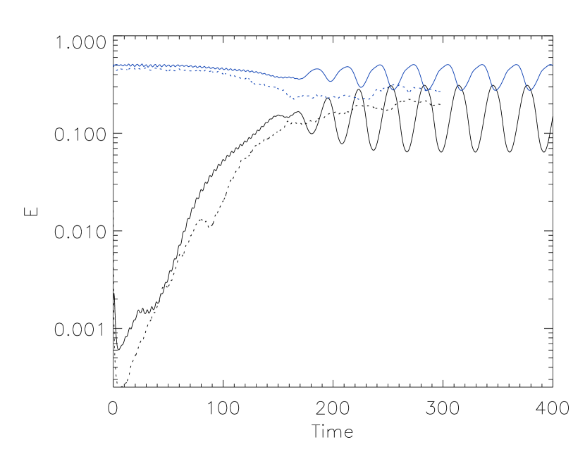
Figure 2: (color online) Time history of kinetic (upper blue curves) and magnetic energy (lower curves) for runs A at low Reynolds (solid lines) and B at high Reynolds (dotted lines) both 6% above threshold.

It is clear that saturation is achieved unsystematically for the high $R_{V}$ run B, with the resulting magnetic energy smaller than the kinetic energy and both in a statistically steady state. The solid lines associated with the lower Reynolds number run A, however, show a systematic, sharp oscillation in both energies, with the maxima of one coinciding with the minima of the other. This is clearly a significantly different behavior from the high $R_{V}$ case, and is only partially understood. Such out-of-phase oscillations have already been observed in the nonlinear regime in constrained geometries, for example using a quasi-geostrophic model for strongly rotating flows (Schaeffer, 2004), or a 2.5D formulation for the Ekman layer instability (Ponty, Gilbert, & Soward, 2001).

In the two simulations presented in Fig. 2 $R_{M}$ is 6% larger than $R_{M}^{c}$, and the growth rates during the kinematic regime are similar. While $\eta$ is one order of magnitude smaller in run B than in run A, the nonlinear saturation in both runs takes place at approximately the same time. In both runs the integral turnover time is approximately the same. This contrasts with dynamos in flows with net helicity, where the nonlinear saturation was shown to occur in a magnetic diffusion time (Brandenburg, 2001) (this diffusion time is of the order of $50$ for run A, and $560$ for run B). Note that although the flow generated by the Taylor-Green force is locally helical, the net helicity of the flow in the entire domain is zero.

The forcing term generating the flow from Eqs. (2) and (3) is initially entirely in the horizontal ($x,y$) directions. It is essentially a vortical flow whose phase oscillates with increasing $z$. The velocity field in Eq. (2) is not, however, a steady state, and vertical ($z$) components develop quickly, leading to an approximately meridional flow to be added to the toroidal one in each cell. A total streamline will resemble the shape of a wire wrapped around the outside of a doughnut, diagonally, which enters the hole of the doughnut at the bottom and emerges at the top.

The amplification process for the magnetic field is difficult to visualize in this geometry. Field lines seem to be sucked into the hole of the doughnut and stretched and twisted in the process. The resulting amplified magnetic flux is then deposited and piled up in the horizontal planes between the cells. This flux, in turn, is the source of the field lines which are further sucked into the holes in the doughnut and amplified. In the kinematic regime, but in a different geometry (including boundary conditions), the amplification of a magnetic field by a similar flow was also discussed in Marié, Burguete, Daviaud, & Léorat (2003); Bourgoin, Odier, Pinton, & Ricard (2004).

Throughout the process, the rate of doing work by the magnetic field on the velocity field originates in the Lorentz force contribution, $-(\mathbf{j}\times\mathbf{B})\cdot\mathbf{v}$. This energy input into the magnetic field is Ohmically dissipated by the $\eta j^{2}$ integral. As the magnetic field grows, the fluid must work harder mechanically, because $\mathbf{j}$ and $\mathbf{B}$ are increasing. Since $F$ is constant, eventually a limit is reached where $\mathbf{v}$ can no longer transfer energy to $\mathbf{B}$ at its previous rate and slows down. At that point, the magnetic energy begins to be transferred in the reverse sense so that $\mathbf{v}$ grows again as $\mathbf{j}$ and $\mathbf{B}$ become weaker. The cyclic nature of the process ensues.

It is revealing to decompose $(\mathbf{j}\times\mathbf{B})\cdot\mathbf{v}$ spectrally and plot the Fourier transform $-\widehat{[(\mathbf{j}\times\mathbf{B})\cdot\mathbf{v}]}_{\mathbf{k}}$ as a function of $k$, as shown in Fig. 3 for run A. The peak near $k=3$ shows that this is the region where the mechanical work is being done to create the magnetic energy. The curve is plotted at four times during a complete oscillation, including $t=344$, where the magnetic energy is at its maximum during the cycle, and $t=360$, where the magnetic energy is at its minimum.

Figure 3: Fourier spectrum of $-(\mathbf{j}\times\mathbf{B})\cdot\mathbf{v}$ for different times for run A for one oscillation.

There is considerable structure to the flow for these low Reynolds number cases, anchored by the driving term in Eq. (2). Figs. 4 show instantaneous plots of the velocity field components along a vertical cut at $x=3\pi/8$ and $y=\pi/4$, as functions of $z$ for run A. This cut corresponds to a line in the $z$ direction displaced (in the $xy$ plane) out of the center line of the vortices imposed by the external Taylor-Green force (corresponding to $x=y=\pi/4$). Plotted in Fig. 4.a is $(v_{y}^{2}+v_{z}^{2})^{1/2}$ vs. $z$, and in Fig. 4.b, $v_{x}$ vs. $z$. In both curves, four different times are shown. In this cut, $v_{x}$ corresponds to the amplitude of the toroidal flow associated with the vortices imposed by the forcing, while $(v_{y}^{2}+v_{z}^{2})^{1/2}$ can be associated with the meridional flow previously defined. Note the mirror symmetries satisfied by the flow. As the oscillations evolve, not only the amplitude of the flow changes, but also the position of the maxima are slightly displaced. The flow geometry will be clarified in more detail in Figs. 5.

Figure 4: (a) $(v_{y}^{2}+v_{z}^{2})^{1/2}$, and (b) $v_{x}$ as a function of $z$ at $x=3\pi/8$ and $y=\pi/4$, and at different times for run A, for one oscillation.

In Figs. 5.a,b are exhibited cross-sectional plots of the velocity field in the plane $z=0$ at two different times for run A. The arrows show the directions of $v_{x}$, $v_{y}$ and the colors indicate the values of $v_{z}$, positive (light) or negative (dark), at the same locations. Note the sixteen vortices imposed by the external Taylor-Green forcing with $k_{0}=2$. The amplitude of these vortices is modulated in $z$, and at $\pi/2$ the same structure is obtained in the flow but with the vortices rotating in the opposite direction. Most of the stretching of magnetic field takes place in these cells. Between these structures, at $z=\pi/4$, stagnation points are present where the magnetic field piles up, as will be shown.

Figs. 5.c,d display similar plots at the plane $y=\pi/4$, with this time $v_{x}$, $v_{z}$ indicated by the arrows, and $v_{y}$ by the color. The regions of alternating color correspond to the cross-section of the vortices imposed by the Taylor-Green forcing. Also the meridional flow can be identified in these cross-sections. However, note that this flow during the cycle is modified by the magnetic field in a more dramatic way than the toroidal flow. As previously shown in Figs. 3 and 4, the Lorentz force mostly opposes the velocity field at large scales. The final effect of the magnetic field on the flow seems to be to suppress small-scale fluctuations, leaving a well-ordered pattern. This effect will be more dramatic at large $R_{V}$, as will be shown in the next subsection.

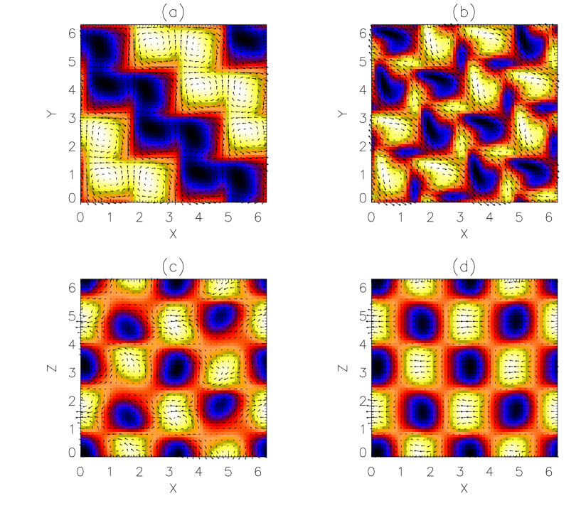
Figure 5: (color online) Upper panels: cross-sectional plots of the velocity field in the plane $z=0$ at (a) $t=352$, and (b) $t=368$, for run A. The arrows show the directions of $v_{x}$, $v_{y}$ and the colors indicate the values of $v_{z}$, positive (light) or negative (dark). Lower panels: cross-sectional plots of the velocity field in the plane $y=\pi/4$ at (c) $t=352$, and (d) $t=368$ ($v_{x}$, $v_{z}$ indicated by the arrows, and $v_{y}$ by the color).

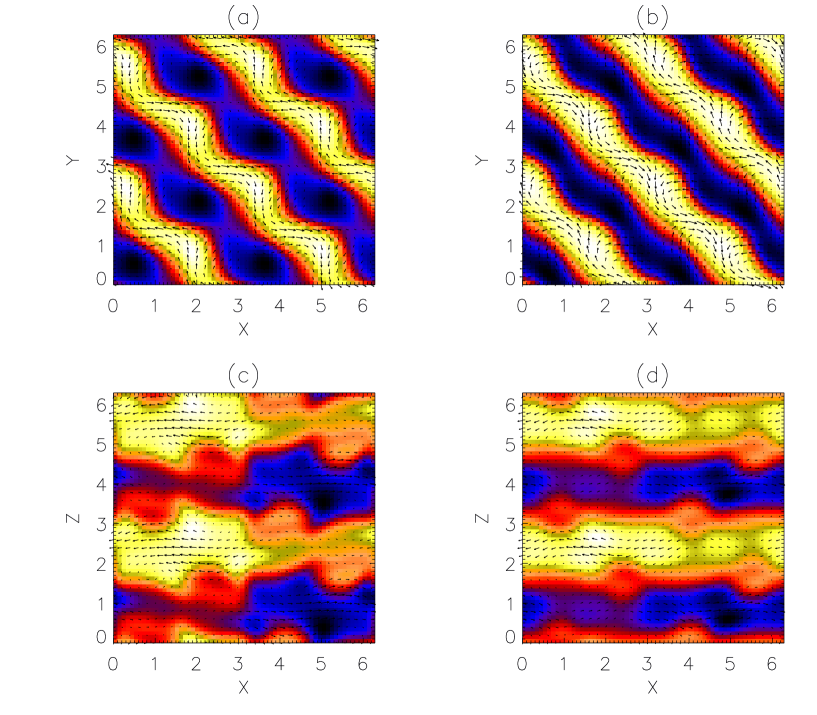
Figure 6: (color online) Upper panels: cross-sectional plots of the magnetic field in the plane $z=0$ at (a) $t=352$, and (b) $t=368$, for run A. Lower panels: cross-sectional plots of the magnetic field in the plane $y=\pi/4$ at (c) $t=352$, and (d) $t=368$. Same conventions than in Fig. 5.

Figs. 6.a,b show the magnetic field in the plane $z=0$ at the same times with the same conventions ($B_{x}$, $B_{y}$ are arrows, $B_{z}$ is indicated by color), again for run A. The stretching of magnetic field lines by the toroidal flow can be observed in these sections. Figs. 6c.d show the magnetic field in the plane $y=\pi/4$ at the same times, and with the same plotting conventions. Note in dark and light colors the horizontal bars where most of the magnetic energy is concentrated. These regions correspond to stagnation planes of the external Taylor-Green forcing.

Fig. 7, finally, shows the magnetic field in the plane $z=0$ at different times for run A. This is a plane between rows of basic cells and is a candidate where the amplified flux “piles up” as previously indicated. It is apparent that the dynamical variation is much less in this plane during the cycle. Also, in Fig. 7 note the presence of locally “dipolar” structures (light and dark regions), centered in each of the Taylor-Green cells. These structures correspond to the almost uniform (and mostly concentrated in the $x$,$y$ plane) magnetic field being sucked into the hole of the doughnut given by the Taylor-Green force.

Figure 7: (color online) cross-sectional plots of the magnetic field in the plane $z=\pi/4$ at (a) $t=352$, and (b) $t=368$, for run A. Same conventions than in Fig. 5.

A more detailed picture of the dynamics of the forced Taylor-Green dynamo at low Reynolds numbers has eluded us, but it is imaginable that in less complex flows a more comprehensive understanding of the low $R_{V}$ non-helical dynamo may be possible.

3.2 High Reynolds numbers and further from threshold

Runs B, B^′ involve higher Reynolds numbers and behave rather differently from runs A, A^′. Fig. 8 contrasts the time histories of the kinetic energies and magnetic energies for run A^′ (solid curves) and run B^′ (dashed), both 20% above threshold. The upper curves are kinetic energies and the lower curves are magnetic energies. It is clear that the B^′ runs saturate at a level of near-equipartition and do not exhibit the oscillatory behavior seen in the lower Reynolds number runs. Run A^′ retains a vestige of the periodic behavior, seen most clearly in the magnetic energy curve which is quasi-periodic or close to “chaotic”. Note the overshooting of the magnetic energy for run B^′ near $t\sim 150$, linked to the large drop in kinetic energy. Note also the similar growth rates (as for runs A and B) although the magnetic diffusivities differ again by almost an order of magnitude.

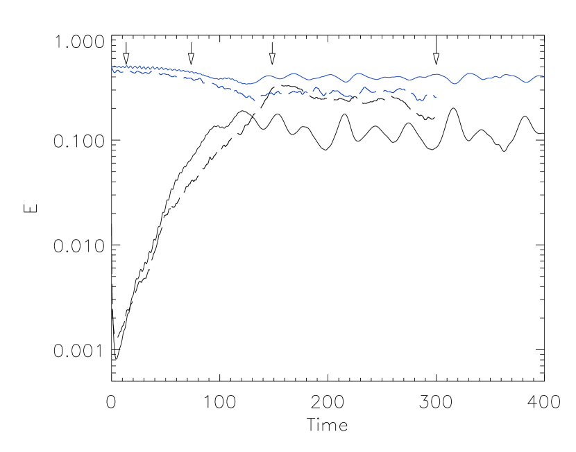
Figure 8: (color online) Time history of kinetic (upper blue curves) and magnetic energy (lower curves) for runs A^′ at low Reynolds (solid lines) and B^′ at high Reynolds (dotted lines), both 20% above threshold. The arrows on the top of the figure represent the times at which the transfer terms displayed in Fig. 11 are evaluated.

During the exponential period of the magnetic energy growth, it is of interest to note that the various Fourier modes all appear to be growing at the same rate in run B^′ (the same effect is observed in run B). This can be seen by separating the Fourier space into “shells” of modes of the same width $\Delta k$. The time histories of these shells are plotted in Fig. 9. In the inset, all the shells have been normalized to have the same amplitudes per $k$-mode at $t=4$, to show that the exponentiation rates up to about $t=30$ are the same or nearly so. This behavior is characteristic of small scale dynamos (Kazantsev, 1967; Brandenburg, 2001). Note that after $t=30$ the shell with $k=2$ seems to start growing faster than the small scale modes. Shortly after this time, the small scales saturate and the large scale magnetic field keeps growing exponentially up to $t=150$.

Figure 9: $B^{2}$ integrated over different shells in Fourier space as a function of time, for run B^′ and $k=1$ (dotted line), $k=2$ (solid) and $k=9,10,11,12$ (dashed lines). The inset shows the evolution at early times, with all the shells normalized to have the same amplitude. The arrows are at the same times as in Fig. 8.

The total kinetic energy spectra (thick lines) and magnetic energy spectra (thin lines) for run B^′ are shown in Fig. 10. Only two kinetic spectra are shown, at times $t=11.4$ and $t=181.8$. At early times, the magnetic energy spectrum peaks at small scales ($k\approx 9$), and the spectrum at large scales seems to satisfy a $k^{3/2}$ power law as already observed for the Taylor-Green flow (Ponty, Mininni, Montgomery, Pinton, Politano, & Pouquet, 2004), and for other flows as well (Haugen, Brandenburg, & Dobler, 2004). The magnetic energy increases from $t=11.4$ to $t=181.8$ and eventually dominates the kinetic energy at the longest wavelength.

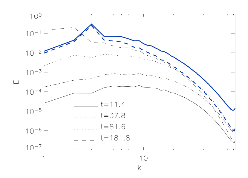
Figure 10: (color online) Kinetic (thick blue lines) and magnetic energy spectra (thin lines) as a function of time for run B^′. Kinetic spectra are only shown at $t=11.4$ and $t=181.8$; note in the latter case, the strong diminution at small scales of the velocity toward magnetic scales.

The appearance of these quasi-dc components of the magnetic field seems to have a profound effect on the short-wavelength kinetic spectral components, depressing them by an order of magnitude, as is also visible from the thick broken line in Fig. 10. The most straightforward interpretation is in terms of what is sometimes called the “Alfvén effect”. The idea is that in incompressible MHD, any nearly spatially uniform, slowly varying, magnetic field forces the small scale excitations to behave like Alfvén waves. In an Alfvén wave, the energy is generally equipartitioned between magnetic field and velocity field, and any mechanism which damps one will damp the other. Since $\eta\gg\nu$ when $P_{M}\ll 1$, the Kolmogorov “inner scale” can be defined entirely in terms of energy dissipation rate and $\eta$, regardless of how much smaller the viscosity is. This was already observed in closure computations of MHD turbulence of low $P_{M}$ Léorat, Pouquet, & Frisch (1981).

One could jump to the conclusion that for $\nu/\eta\ll 1$, the dynamo process will behave as if $P_{M}$ were of $\mathcal{O}(1)$ (see Yousef, Brandenburg, & Rüdiger (2003) for different simulations supporting this conclusion). This is certainly inappropriate in the formation, or “kinematic,” phase, when the magnetic field is small but amplifying and there is no quasi-dc magnetic field to enforce the necessary approximate equipartition at small scales. This conclusion can also apply in more complex systems, such as during the reversals of the Earth’s dynamo.

The central role played by the $-\mathbf{v}\cdot(\mathbf{j}\times\mathbf{B})$ term by which energy is injected into the magnetic field can be clarified by plotting the transfer functions $T(k)$ for the magnetic field and velocity field as functions of $k$ at different times.

The energy transfer function

$$T(k)=T_{V}(k)+T_{M}(k),$$ (9)

represents the transfer of energy in $k$-space, and is obtained by dotting the Fourier transform of the nonlinear terms in the momentum equation (2) and in the induction equation (3), by the Fourier transform of $\mathbf{v}$ and $\mathbf{B}$ respectively. It also satisfies

$$0=\int_{0}^{\infty}{T(k^{\prime})\,\textrm{d}k^{\prime}},$$ (10)

because of energy conservation by the non-linear terms; one can also define

$$\Pi(k)=\int_{0}^{k}{T(k^{\prime})\,\textrm{d}k^{\prime}},$$ (11)

where $\Pi(k)$ is the energy flux in Fourier space. In equation (9), $T_{V}(k)$ is the transfer of kinetic energy

$$T_{V}(k)=\int{\hat{\mathbf{v}}_{\mathbf{k}}\cdot\left[-\widehat{\left(\mbox{\boldmath$\omega$}\times\mathbf{v}\right)}_{\mathbf{k}}+\widehat{\left(\mathbf{j}\times\mathbf{B}\right)}_{\mathbf{k}}\right]^{*}\,\textrm{d}\Omega_{\mathbf{k}}},$$ (12)

where the hat denotes Fourier transform, the asterisk complex conjugate, and $d\Omega_{\mathbf{k}}$ denotes integration over angle in Fourier space. In this equation and the following, it is assumed that the complex conjugate part of the integral is added to obtain a real transfer function.

The transfer of magnetic energy is given by

$$T_{M}(k)=\int{\hat{\mathbf{B}}_{\mathbf{k}}\cdot\nabla\times\widehat{\left(\mathbf{v}\times\mathbf{B}\right)}_{\mathbf{k}}^{*}\,\textrm{d}\Omega_{\mathbf{k}}},$$ (13)

and we can also define the transfer of energy due to the Lorentz force

$$T_{L}(k)=\int{\hat{\mathbf{v}}_{\mathbf{k}}\cdot\widehat{\left(\mathbf{j}\times\mathbf{B}\right)}_{\mathbf{k}}^{*}\,\textrm{d}\Omega_{\mathbf{k}}}.$$ (14)

Note that this latter term is part of $T_{V}(k)$; it gives an estimation of the alignment between the velocity field and the Lorentz force at each Fourier shell (as shown previously in Fig. 3). Also, this term represents energy that is transfered from the kinetic reservoir to the magnetic reservoir [in the steady state, the integral over all $k$ of $T_{L}(k)$ is equal to the magnetic energy dissipation rate, as follows from eq. (3)].

Fig. 11 shows the transfer functions: $T(k;t=0)$ (which corresponds to the total energy transfer in the hydrodynamic simulation, since the magnetic seed has just been introduced); $T(k)$ (which is the total energy transfer); $T_{V}(k)$; $T_{M}(k)$; and $-T_{L}(k)$, as functions of $k$ for four different times for run B^′. A gap in one of the spectra indicates (since the plotting is logarithmic) that it has changed sign. It is apparent that the dominant transfer is always in the vicinity of the forcing band, although it is quite spread over all wavenumbers in the inertial range at all times. It is also apparent that at the later times, most of the transfer is magnetic transfer, in which, of course, the velocity field must participate (see eq. 13).

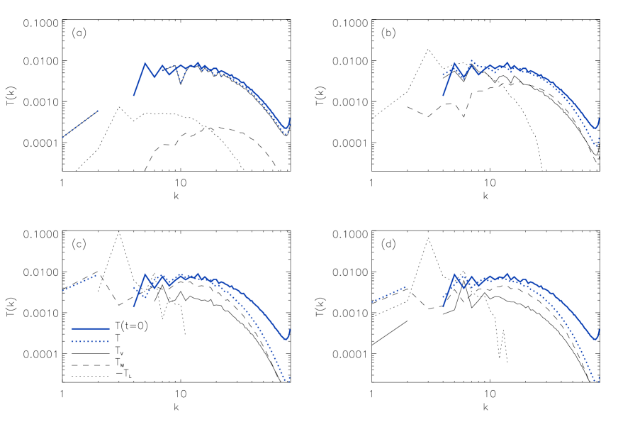
Figure 11: (color online) Transfer of energy in Fourier space in run B^′, at (a) $t=13.5$ in the kinematic regime (see Fig. 9), (b) $t=73.5$ at the end of the kinematic regime, (c) $t=148.5$ at the time of rapid growth of the $k=2$ shell, and (d) $t=300$. In all the figures, the total transfer at $t=0$ (thick blue solid line) is shown as a reference (which corresponds to the $\mathbf{B}=0$ case); dotted, dashed, and solid lines represent transfer as indicated in (c). Since $T_{L}$ is negative at most $k$, $-T_{L}$ is shown.

During the kinematic regime (Fig. 11.a), the kinetic energy transfer $T_{V}(k)$ is almost equal to the total transfer. Note that the Lorentz force opposes the velocity field at almost all scales, and $-T_{L}(k)$ is approximately constant between $k\approx 3$ and $k\approx 12$; all these modes in the magnetic energy grow with the same growth rate (see Fig. 9). The statistically anti-parallel alignment between the Lorentz force and the velocity field follows from Lenz’s law: the electromagnetic force associated with the current induced by the motion of the fluid has to oppose the change in the field in order to ensure the conservation of energy. Of course, the amplified magnetic field is getting its energy from the velocity field. Note that then $-T_{L}(k)$ can be used as a signature of the scale at which the magnetic field extracts energy from the velocity field (compare this result with the low $R_{V}$ case, where $-T_{L}(k)$ peaks at $k=3$ both in the kinematic regime and in the nonlinear stage). As its counterpart, the transfer of magnetic energy $T_{M}(k)$ represents both the scales where magnetic field is being created by stretching, and the nonlinear transfer of energy to smaller scales. $T_{L}(k)$ is peaked at wavenumbers larger than $T_{M}(k)$; the magnetic field extracts energy from the flow at all scales between $k\approx 3$ and $k\approx 12$, and this energy turns into magnetic energy at smaller scales through a cascade process.

As time evolves and the magnetic small scales saturate, a peak in $-T_{L}(k)$ grows at $k=3$ (Fig. 11.b). At the same time, the transfer of kinetic energy $T_{V}(k)$ at small scales is quenched (compared with Fig. 11.a, it has diminished in amplitude by almost one order of magnitude). This time corresponds to the time where a large scale ($k=2$) magnetic field starts to grow (see Figs. 9 and 10). In the saturated regime (Figs. 11.c,d) $T_{L}(k)$ is negative at large scales and peaks strongly at $k=3$ at late times. As previously mentioned, this term represents also energy transfered from the kinetic reservoir to the magnetic reservoir. As a result, a substantial fraction of the injected energy is seen to be transfered to the magnetic field in the injection band ($k=3$), and then most of that energy is carried to small scales by the magnetic field ($T_{M}(k)>T_{V}(k)$ up to the magnetic dissipation scale in the steady state, Figs. 11.c,d). A counterpart of this dynamic was observed in Haugen, Brandenburg, & Dobler (2004), where it was noted by examination of global quantities that most of the energy injected in the saturated regime of the dynamo is dissipated by the magnetic field. Similarly in run B we find that $\left<\nu\omega^{2}\right>/\left<\eta j^{2}\right>\approx 0.4$ at $t=300$. This explains the drop in the kinetic energy spectrum at late times (Fig. 10). Note also that the transfer functions $T_{V}(k)$ and $T_{M}(k)$ drop together at small scales.

In summary, during the kinematic regime the magnetic field is amplified in a broad region of $k$-space, while in the nonlinear phase most of the amplification takes place at large scales. This contrasts with the low $R_{V}$, $P_{M}\approx 1$ case, where the magnetic energy grows at large scales ($k=2$) from the beginning of the kinematic dynamo phase, the small scales being undeveloped.

Finally, we may ask if anything remains visible of any pattern enforced by the forcing function $F\mathbf{v}_{TG}$ in the higher Reynolds number runs. Fig. 12 suggests that the answer is yes. It is a plot for run B^′ of a cross section ($y=\pi/4$) in which the magnetic field strength is exhibited: arrows denote components in the plane and colors denote components normal to the plane. The left panel is at $t=70$, and the right panel is at $t=300$. The two horizontal bands are associated with the stagnation planes of the Taylor-Green forcing.

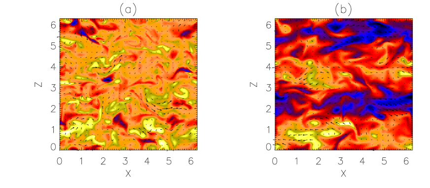
Figure 12: (color online) Cross-sectional plots of the magnetic field in the plane $y=\pi/4$ at (a) $t=70$, and (b) $t=300$ ($B_{x}$, $B_{z}$ indicated by the arrows, and $B_{y}$ by the color) for run B^′.

While at $t=70$ the magnetic field is mostly at small scale, at $t=300$ a pattern reminiscent of the low $R_{V}$ case (Fig. 6.d) can be clearly seen, albeit more turbulent. This is the result of the suppression of small scales by the magnetic field. While in the kinematic regime the magnetic field grows under a broad kinetic energy spectrum, when the large scale magnetic field starts to grow the small scale velocity field fluctuations are quenched (Figs. 10 and 11), and the large scale pattern reappears. This “clean up” effect was also observed in Brandenburg, Bigazzi, & Subramanian (2001), but there both the large scale pattern in the flow and the turbulent fluctuations at small scale were imposed, while here the turbulent fluctuations are the result of the large scale external force and high values of $R_{V}$.

4 DISCUSSION AND SUMMARY

The oscillatory behavior exemplified in Fig. 2 is not without precedent. It is common for a pulsation to occur in a faucet when the pressure drop is such as to cause the flow of the water to be close to a speed near the threshold of the transition to turbulence. The developing turbulence acts as an eddy viscosity to reduce the Reynolds number back into the laminar regime. As the turbulence then subsides, the flow accelerates until the flow speed is again in the unstable regime and the cycle repeats.

A few years ago (Shan and Montgomery, 1993a, b), a similarly quasi-periodic behavior was observed in an MHD problem which might be considered an opposite limit of the dynamo problem. A quiescent, periodic circular cylinder of magnetofluid was supported by an external axial magnetic field and carried an axial current driven by an applied axial voltage. By increasing the axial current, it was possible to cross a stability boundary for the onset of mechanical motion. The unstable modes were helical, as regards the behavior of $\mathbf{v}$ and $\mathbf{B}$. The resulting $-\mathbf{v}\times\mathbf{B}$ axial electromotive force opposed the sense of the applied electric field and constituted an effective increase in the resistance of the column. When the disturbances grew large enough, the total axial current was reduced back below the stability threshold, causing the magnetofluid to re-laminarize itself. A cyclic oscillation in magnetic and kinetic energy resulted, with the larger energy being magnetic, which in many ways resembles qualitatively the oscillations exhibited in Fig. 2, except that the magnetic energy remained larger: a sort of “inverse dynamo” problem.

In the high Reynolds case, part of this dynamic persists. In the steady state of the dynamo, the large scale magnetic field forces small scale excitations to be equipartitioned between magnetic field and velocity field, and both fields are damped at almost the same scale. As a result, velocity fluctuations are strongly suppressed and at late times similar structures can be recognized in the magnetic field in both the low and high Reynolds simulations.

In all cases, a statistically anti-parallel alignment between the Lorentz force and the velocity field was observed by examination of nonlinear transfer in Fourier space, stressing the different dynamics at different scales. This alignment is more significant at scales where the magnetic field is being amplified, and follows from Lenz’s law applied to a conducting fluid and the conservation of the total energy.

It is clear that there are many distinct dynamo behaviors, depending upon the parameters and the nature and scale of the mechanical forcing. It should not be inferred that the oscillatory behavior shown in Fig. 2 is more generic than it is. Different kinds of oscillations can appear as the forcing amplitude is varied, for example, or as the timing of the seed magnetic field’s introduction is varied. The oscillations can acquire different qualitative features as these features are changed. It may be expected that, once turbulent computations in geometries other than rectangular periodic ones are undertaken, still further variety may occur.

References

- Archontis, Dorch, & Nordlund (2003) Archontis, V., Dorch, S.B.F., & Nordlund, Å. 2003, Astron. & Astrophys., 410, 759
- Brandenburg (2001) Brandenburg, A. 2001, ApJ, 550, 824
- Brandenburg, Bigazzi, & Subramanian (2001) Brandenburg, A., Bigazzi, A., & Subramanian, K. 2001, MNRAS, 325, 685
- Bourgoin, Odier, Pinton, & Ricard (2004) Bourgoin, M., Odier, P., Pinton, J.-F., & Ricard, Y. 2004, Phys. Fluids, 16, 2529
- Haugen, Brandenburg, & Dobler (2004) Haugen, N.E., Brandenburg, A., & Dobler, W. 2004, Phys. Rev. E, 70, 016308
- Kazantsev (1967) Kazanstev, A.P. 1967, Sov. Phys. JETP, 26, 1031
- Léorat, Pouquet, & Frisch (1981) Léorat, J., Pouquet, A., & Frisch, U. 1981, J. Fluid. Mech., 104, 419
- Marié, Burguete, Daviaud, & Léorat (2003) Marié, L., Burguete, J., Daviaud, F., & Léorat, J. 2003, Eur. Phys. J., B33, 469
- Moffatt (1978) Moffatt, H.K. 1978, Magnetic field generation in electrically conducting fluids (Cambridge: Cambridge University Press)
- Morf, Orszag, & Frisch (1980) Morf, R.H., Orszag, S.A., & Frisch, U. 1980, Phys. Rev. E, 44, 572
- Nore, Brachet, Politano, & Pouquet (1997) Nore, C., Brachet, M.E., Politano, H., & Pouquet, A. 1997, Phys. Plasmas, 4, 1
- Pelz, Yakhot, Orszag, Shtilman, & Levich (1985) Pelz, R.B., Yakhot, V., Orszag, S.A., Shtilman, L., & Levich, E. 1985, Phys. Rev. E, 54, 2505
- Ponty, Gilbert, & Soward (2001) Ponty, Y., Gilbert, A.D., & Soward, A.M. 2001, in Dynamo and Dynamics, a Mathematical Challenge, eds. P. Chossat, D. Armbruster, & I. Oprea, (Boston: Kluwer Acad. Pub.), 261
- Ponty, Mininni, Montgomery, Pinton, Politano, & Pouquet (2004) Ponty, Y., Mininni, P.D., Montgomery, D.C., Pinton, J.-F., Politano, H., & Pouquet, A. 2004, Phys. Rev. E(submitted); arXiv:physics/0410046
- Taylor & Green (1937) Taylor, G.I. & Green, A.E. 1937, Proc. Roy. Soc. Lond., A158, 499
- Schaeffer (2004) Schaeffer, N. 2004, “Instabilités, turbulence et dynamo dans une couche de fluide cisaillée en rotation rapide: importance de l’aspect ondulatoire”, Thèse, Université Joseph Fourier (Grenoble)
- Yousef, Brandenburg, & Rüdiger (2003) Yousef, T.A., Brandenburg, A., & Rüdiger, G. 2003, Astron. & Astrophys., 411, 321
- Shan and Montgomery (1993a) Shan, X. & Montgomery, D. 1993a, Plasma Phys. and Contr. Fusion, 35, 619
- Shan and Montgomery (1993b) Shan, X. & Montgomery, D. 1993b, Plasma Phys. and Contr. Fusion, 35, 1019