Particle-In-Cell simulations of circularly polarised Alfvén wave phase mixing: a new mechanism for electron acceleration in collisionless plasmas

In this work we used Particle-In-Cell simulations to study the interaction of circularly polarised Alfvén waves with one dimensional plasma density inhomogeneities transverse to the uniform magnetic field (phase mixing) in collisionless plasmas. In our preliminary work we reported discovery of a new electron acceleration mechanism, in which progressive distortion of the Alfvén wave front, due to the differences in local Alfvén speed, generates an oblique (nearly parallel to the magnetic field) electrostatic field. The latter accelerates electrons through the Landau resonance. Here we report a detailed study of this novel mechanism, including: (i) analysis of broadening of the ion distribution function due to the presence of Alfvén waves and (ii) the generation of compressive perturbations due to both weak non-linearity and plasma density inhomogeneity. The amplitude decay law in the inhomogeneous regions, in the kinetic regime, is demonstrated to be the same as in the MHD approximation described by Heyvaerts and Priest (1983).

1 Introduction

The study of the interaction of Alfvén waves (AWs) with plasma inhomogeneities is important for both astrophysical and laboratory plasmas. This is because both AWs and inhomogeneities often coexist in these physical systems. AWs are believed to be good candidates for plasma heating, energy and momentum transport. On the one hand, in many physical situations AWs are easily excitable (e.g. through convective motion of the solar interior) and thus they are present in a number of astrophysical systems. On the other hand, these waves dissipate due to the shear viscosity as opposed to compressive fast and slow magnetosonic waves which dissipate due to the bulk viscosity. In astrophysical plasmas shear viscosity is extremely small as compared to bulk viscosity. Hence, AWs are notoriously difficult to dissipate. One of the possibilities to improve AW dissipation is to introduce progressively decreasing spatial scales, $\delta l\to 0$, into the system (recall that the classical dissipation is $\propto\delta l^{-2}$). Heyvaerts and Priest have proposed (in the astrophysical context) one such mechanism, called AW phase mixing (Heyvaerts & Priest 1983). It occurs when a linearly polarised AW propagates in the plasma with a one dimensional density inhomogeneity transverse to the uniform magnetic field. In such a situation the initially plane AW front is progressively distorted because of different Alfvén speeds across the field. This creates progressively stronger gradients across the field (in the inhomogeneous regions the transverse scale collapses to zero), and thus in the case of finite resistivity, dissipation is greatly enhanced. Hence, it is believed that phase mixing can provide significant plasma heating. Phase mixing could be also important for laboratory plasmas. Hasegawa & Chen (1974) proposed the heating of collisionless plasma by utilising spatial phase mixing by shear Alfvén wave resonance and discussed potential applications to toroidal plasma. A significant amount of work has been done in the context of heating open magnetic structures in the solar corona (Heyvaerts & Priest 1983; Nocera et al. 1986; Parker 1991; Nakariakov et al. 1997; DeMoortel et al. 2000; Botha et al. 2000; Tsiklauri et al. 2001; Hood et al. 2002; Tsiklauri & Nakariakov 2002; Tsiklauri et al. 2002, 2003). All phase mixing studies so far have been performed in the MHD approximation, however, since the transverse scales in the AW collapse progressively to zero, the MHD approximation is inevitably violated. This happens when the transverse scale approaches the ion gyro-radius $r_{i}$ and then electron gyro-radius $r_{e}$. Thus, we proposed to study the phase mixing effect in the kinetic regime, i.e. we go beyond a MHD approximation. Preliminary results were reported in Tsiklauri et al. (2005), where we discovered a new mechanism for the acceleration of electrons due to wave-particle interactions. This has important implications for various space and laboratory plasmas, e.g. the coronal heating problem and acceleration of the solar wind. In this paper we present a full analysis of the discovered effect including an analysis of the broadening of the ion distribution function due to the presence of Alfvén waves and the generation of compressive perturbations due to both weak non-linearity and plasma density inhomogeneity.

2 The model

We used 2D3V, the fully relativistic, electromagnetic, particle-in-cell (PIC) code with MPI parallelisation, modified from the 3D3V TRISTAN code (Buneman 1993, p.67). The system size is $L_{x}=5000\Delta$ and $L_{y}=200\Delta$, where $\Delta(=1.0)$ is the grid size. The periodic boundary conditions for $x$- and $y$-directions are imposed on particles and fields. There are about 478 million electrons and ions in the simulation. The average number of particles per cell is 100 in low density regions (see below). The thermal velocity of electrons is $v_{th,e}=0.1c$ and for ions is $v_{th,i}=0.025c$. The ion to electron mass ratio is $m_{i}/m_{e}=16$. The time step is $\omega_{pe}\Delta t=0.05$. Here $\omega_{pe}$ is the electron plasma frequency. The Debye length is $v_{th,e}/\omega_{pe}=1.0$. The electron skin depth is $c/\omega_{pe}=10\Delta$, while the ion skin depth is $c/\omega_{pi}=40\Delta$. Here $\omega_{pi}$ is the ion plasma frequency. The electron Larmor radius is $v_{th,e}/\omega_{ce}=1.0\Delta$, while the same for ions is $v_{th,i}/\omega_{ci}=4.0\Delta$. The external uniform magnetic field, $B_{0}(=1.25)$, is in the $x$-direction and the initial electric field is zero. The ratio of electron cyclotron frequency to the electron plasma frequency is $\omega_{ce}/\omega_{pe}=1.0$, while the same for ions is $\omega_{ci}/\omega_{pi}=0.25$. The latter ratio is essentially $V_{A}/c$ – the Alfvén speed normalised to the speed of light. Plasma $\beta=2(\omega_{pe}/\omega_{ce})^{2}(v_{th,e}/c)^{2}=0.02$. Here all plasma parameters are quoted far away from the density inhomogeneity region. The dimensionless (normalised to some reference constant value of $n_{0}=100$ particles per cell) ion and electron density inhomogeneity is described by

$${n_{i}(y)}={n_{e}(y)}=1+3\exp\left[-\left(\frac{y-100\Delta}{50\Delta}\right)^{6}\right]\equiv F(y).$$ (1)

This means that in the central region (across the $y$-direction), the density is smoothly enhanced by a factor of 4, and there are the strongest density gradients having a width of about ${50\Delta}$ around the points $y=51.5\Delta$ and $y=148.5\Delta$. The background temperature of ions and electrons, and their thermal velocities are varied accordingly

$${T_{i}(y)}/{T_{0}}={T_{e}(y)}/{T_{0}}=F(y)^{-1},$$ (2)

$${v_{th,i}}/{v_{i0}}={v_{th,e}}/{v_{e0}}=F(y)^{-1/2},$$ (3)

such that the thermal pressure remains constant. Since the background magnetic field along the $x$-coordinate is also constant, the total pressure remains constant too. Then we impose a current of the following form

$${\partial_{t}E_{y}}=-J_{0}\sin(\omega_{d}t)\left(1-\exp\left[-(t/t_{0})^{2}\right]\right),$$ (4)

$${\partial_{t}E_{z}}=-J_{0}\cos(\omega_{d}t)\left(1-\exp\left[-(t/t_{0})^{2}\right]\right).$$ (5)

Here $\omega_{d}$ is the driving frequency which was fixed at $\omega_{d}=0.3\omega_{ci}$. This ensures that no significant ion-cyclotron damping is present. Also, $\partial_{t}$ denotes the time derivative. $t_{0}$ is the onset time of the driver, which was fixed at $50/\omega_{pe}$ i.e. $3.125/\omega_{ci}$. This means that the driver onset time is about 3 ion-cyclotron periods. Imposing such a current on the system results in the generation of left circularly polarised AW, which is driven at the left boundary of simulation box and has spatial width of $1\Delta$. The initial amplitude of the current is such that the relative AW amplitude is about 5 % of the background (in the low density homogeneous regions), thus the simulation is weakly non-linear.

3 Main results

Because no initial (perpendicular to the external magnetic field) velocity excitation was imposed in addition to the above specified currents (cf. Tsiklauri & Nakariakov (2002); DelZanna et al. (2001); Turkmani & Torkelsson (2003, 2004)), the circularly polarised AW excited (driven) at the left boundary is split into two circularly polarised AWs which travel in opposite directions. The dynamics of these waves as well as other physical quantities is shown in Fig. 1. (cf. Fig. 1 from Tsiklauri et al. (2005) where $B_{z}$ and $E_{y}$, the circularly polarised Alfvén wave components, were shown for three different times). A typical simulation, untill $t=875/\omega_{ce}=54.69/\omega_{ci}$ takes about 8 days on the parallel 32 dual 2.4 GHz Xeon processors. It can be seen from the figure that because of the periodic boundary conditions, a circularly polarised AW that was travelling to the left, reappeared on the right side of the simulation box. The dynamics of the AW ($B_{z},E_{y}$) progresses in a similar manner as in the MHD, i.e. it phase mixes (Heyvaerts & Priest 1983). In other words, the middle region (in $y$-coordinate), i.e. $50\Delta\leq y\leq 150\Delta$, travels slower because of the density enhancement (note that $V_{A}(y)\propto 1/\sqrt{n_{i}(y)}$). This obviously causes a distortion of initially plain wave front and the creation of strong gradients in the regions around $y\approx 50$ and $150$. In the MHD approximation when resistivity, $\eta$, is finite, the AW is strongly dissipated in these regions. This effectively means that the outer and inner parts of the travelling AW are detached from each other and propagate independently. This is why the effect is called phase mixing – after a long time (in the case of developed phase mixing), phases in the wave front become effectively uncorrelated. Before Tsiklauri et al. (2005), it was not clear what to expect from our PIC simulation. The code is collisionless and there are no sources of dissipation in it (apart from the possibility of wave-particle interactions). It is evident from Fig. 1 that in the developed stage of phase mixing ($t=54.69/\omega_{ci}$), the AW front is substantially damped in the strongest density gradient regions. Contrary to the AW ($B_{z}$ and $E_{y}$) dynamics we do not see any phase mixing for $B_{y}$ and $E_{z}$. The latter two behave similarly. It should be noted that $E_{z}$ contains both driven (see Eq.(4) above) and non-linearly generated fast magnetosonic wave components, with the former being dominant over the latter. Since $B_{x}$ is not driven, and initially its perturbations are absent, we see only non-linearly generated slow magnetosonic perturbations confined to the regions of strongest density gradients (around $y\approx 50$ and $150$). Note that these also have rapidly decaying amplitude. Also, we gather from Fig. 1 that the density perturbation ($\approx 10$%) which is also generated through the weak non-linearity is present too. These are propagating density oscillations with variation both in overall magnitude (perpendicular to the figure plane) and across the $y$-coordinate, and they are mainly confined to the strongest density gradients regions (around $y\approx 50$ and $150$). Note that dynamics of $B_{x},B_{y}$ and $B_{z}$ with appropriate geometrical switching (because in our geometry the uniform magnetic field lies along the $x$-coordinate) is in qualitative agreement with Botha et al. (2000) (cf their Fig. 9). The dynamics of remaining $E_{x}$ component is treated separately in the next figure. It is the inhomogeneity of the medium $n_{i}(y)$, $V_{A}(y)$, i.e. $\partial/\partial y\not=0$, is the cause of weakly non-linear coupling of the AWs to the compressive modes (see Nakariakov et al. (1997); Tsiklauri et al. (2001) for further details).

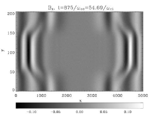
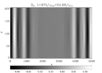
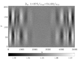
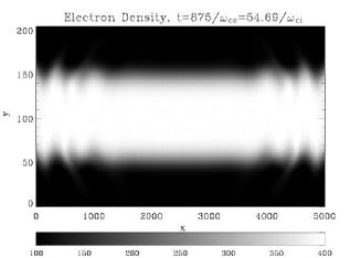
Figure 1: Contour (intensity) plots of electromagnetic field components and electron density at time $t=54.69/\omega_{ci}$ (developed stage of phase mixing). The phase mixed Alfvén wave components are $B_{z}$ and $E_{y}$. The excitation source is at the left boundary. Because of periodic boundary conditions, the left-propagating AW re-appears from the right side of the simulation box. Note how the (initially plain) AW is stretched because of differences in local Alfvén speed across the $y$-coordinate. Significant ($\approx 10$%) density fluctuations can be seen.

In Fig. 2 we try to address the question of where the AW energy went? (as we saw strong decay of AWs in the regions of strong density gradients). Thus in Fig. 2 we plot $E_{x}$, the longitudinal electrostatic field, and electron phase space ($V_{x}/c$ vs. $x$ and $V_{x}/c$ vs. $y$) for different times. In the regions around $y\approx 50$ and $150$, for later times, a significant electrostatic field is generated. This is the consequence of stretching of the AW front in those regions because of the difference in local Alfvén speed. In the middle column of this figure we see that exactly in those regions where $E_{x}$ is generated, many electrons are accelerated along $x$-axis. We also gather from the right column that for later times ($t=54.69/\omega_{ci}$), the number of high velocity electrons is increased around the strongest density gradient regions (around $y\approx 50$ and $150$). Thus, the generated $E_{x}$ field is somewhat oblique (not exactly parallel to the external magnetic field). Hence, we conclude that the energy of the phase-mixed AW goes into acceleration of electrons. Line plots of $E_{x}$ show that this electrostatic field is strongly damped, i.e. the energy is channelled to electrons via Landau damping.

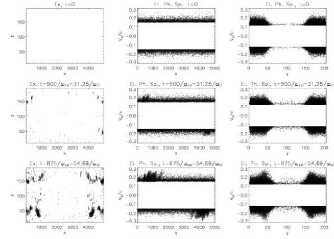
Figure 2: Left column: contour plots of the generated electrostatic field $E_{x}$ nearly parallel to the external magnetic field at instances: $t=(0,31.25,54.69)/\omega_{ci}$. Central column: $V_{x}/c$ versus $x$ of electron phase space at the same times. To reduce figure size, only electrons with $V_{x}>0.15c$ were plotted. Right column: $V_{x}/c$ versus $y$ of electron phase space at the same times. Only electrons with $V_{x}>0.12c$ were plotted (note the dip in the middle due to the density inhomogeneity across $y$-coordinate).

In Fig. 3 we investigate ion phase space ($V_{z}/c$ vs. $x$ and $V_{z}/c$ vs. $y$) for the different times. The reason for choice of $V_{z}$ will become clear below. We gather from this plot that in $V_{z}/c$ vs. $x$ phase space, clear propagating oscillations are present (left column). These oscillations are of the incompressible, Alfvénic ”kink” type, i.e. for those $x$s where there is an increase of greater positive velocity ions, there is also a corresponding decrease of lower negative velocity ions. In the $V_{z}/c$ vs. $y$ plot we also see no clear acceleration of ions.

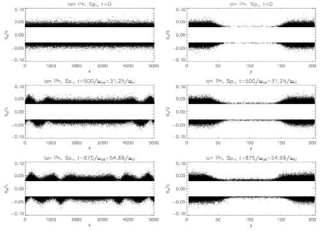
Figure 3: Left column: $V_{z}/c$ versus $x$ of ion phase space at instances: $t=(0,31.25,54.69)/\omega_{ci}$. Right column: $V_{z}/c$ versus $y$ of ion phase space at the same times. Only ions with $V_{z}>0.03c$ are plotted (note the dip in the middle due to the density inhomogeneity across the $y$-coordinate).

We next look at the distribution functions of electrons and ions before and after the phase mixing took place. In Fig. 4 we plot distribution functions of electrons and ions at $t=0$ and $t=54.69/\omega_{ci}$. Note that at $t=0$ the distribution functions do not look as purely Maxwellian because of the fact that the temperature varies across the $y$-coordinate (to keep total pressure constant) and the graphs are produced for the entire simulation domain. Also, note that for electrons in $f(V_{x})$ there is a substantial difference at $t=54.69/\omega_{ci}$ to its original form because of the aforementioned electron acceleration. We see that the number of electrons having velocities $V_{x}=\pm(0.1-0.3)c$ is increased. Note that the acceleration of electrons takes place mostly along the external magnetic field (along the $x$-coordinate). Thus, very little electron acceleration occurs for $V_{y}$ or $V_{z}$ (solid and dotted curves practically overlap each other). For the ions the situation is different: we see broadening of the ion velocity distribution functions in $V_{z}$ and $V_{y}$ (that is why we have chosen to present the $V_{z}$ component of ion phase space in Fig. 3).

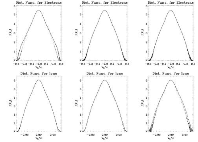
Figure 4: All three components of the distribution functions of electrons (top row) and ions (bottom row) at $t=0$ (dotted curves) and $t=54.69/\omega_{ci}$ (solid curves), i.e. for the developed stage of phase mixing.

The reason for this broadening of the ion distribution function becomes clear in Fig. 5 where we plot kinetic energy $x,y,z$ components ($\propto V_{x,y,z}^{2}$) and total kinetic energies for electrons (top row) and ions (bottom row). For ions we gather that $y$ and $z$ components of the kinetic energy (bottom left figure) oscillate in anti-phase and their oscillatory part perfectly cancels out in the total energy (bottom right figure). Thus, the broadening of the $y$ and $z$ components of the ion velocity distribution functions is due to the presence of AWs (usual wave broadening, which is actually observed e.g. in the solar corona and solar wind, Belcher & Davis (1971); Smith et al. (1995); Bavassano et al. (2000)), and hence there is no ion acceleration present. Note that $y$ and $z$ components and hence total kinetic energy of ions is monotonously increasing due to continuous AW driving. Note that no significant motion of ions along the field is present. For electrons, on the other hand, we see a significant increase of the $x$ component (along the magnetic field) of kinetic energy which is due to the new electron acceleration mechanism discovered by us (cf. Fig.10). Note that for ions the $y$ component reaches lower values (than the $z$ component) because of lower AW velocity in the middle part of the simulation domain.

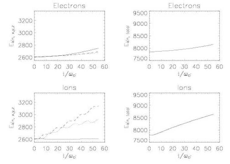
Figure 5: Top row: kinetic energies (calculated by $x$ (solid), $y$ (dotted), $z$ (dashed) velocity (squared) components) of electrons (left), and total kinetic energy for electrons (right) as a function of time. Bottom row: As above but for ions. The units on $y$-axis are arbitrary.

The next step is to check whether the increase in electron velocities really comes from the resonant wave particle interactions. For this purpose in Fig. 6, left panel, we plot two snapshots of the Alfvén wave $B_{z}(x,y=148)$ component at instances $t=54.69/\omega_{ci}$ (solid line) and $t=46.87/\omega_{ci}$ (dotted line). The distance between the two upper leftmost peaks (which is the distance travelled by the wave in the time span between the snapshots) is about $\delta L=150\Delta=15(c/\omega_{pe})$. The time difference between the snapshots is $\delta t=7.82/\omega_{ci}$. Thus, the measured AW speed at the point of the strongest density gradient ($y=148$) is $V_{A}^{M}=\delta L/\delta t=0.12c$. We can also work out the Alfvén speed from theory. In the homogeneous low density region the Alfvén speed was set to be $V_{A}(\infty)=0.25c$. From Eq.(1) it follows that for $y=148$ the density is increased by a factor of $2.37$ which means that the Alfvén wave speed at this position is $V_{A}(148)=0.25/\sqrt{2.37}c=0.16c$. The measured ($0.12c$) and calculated ($0.16c$) Alfvén speeds in the inhomogeneous regions do not coincide. This is probably because the AW front is decelerated (due to momentum conservation) as it passes on energy and momentum to the electrons in the inhomogeneous regions (where electron acceleration takes place). However, this possibly is not the case if wave-particle interactions play the same role as dissipation in MHD (Sagdeev & Galeev 1969): Then wave-particle interactions would result only in the decrease of the AW amplitude (dissipation) and not in its deceleration. If we compare these values to Fig. 4 (top left panel for $f(V_{x})$), we deduce that these are the velocities $>0.12c$ above which electron numbers with higher velocities are greatly increased. This deviation peaks at about $0.25c$ which, in fact, corresponds to the Alfvén speed in the lower density regions. This can be explained by the fact the electron acceleration takes place in wide regions (cf. Fig. 2) along and around $y\approx 148$ (and $y\approx 51$) – hence the spread in the accelerated velocities. In Fig. 6 we also plot a visual fit curve (dashed line) to quantify the amplitude decay law for the AW (at $t=54.69/\omega_{ci}$) in the strongest density inhomogeneity region. The fitted (dashed) cure is represented by $0.056\exp\left[-\left({x}/{1250}\right)^{3}\right]$. There is a surprising similarity of this fit with the MHD approximation results. Heyvaerts & Priest (1983) found that for large times (developed phase mixing), in the case of a harmonic driver, the amplitude decay law is given by $\propto\exp\left[-\left(\frac{\eta\omega^{2}V_{A}^{\prime 2}}{6V_{A}^{5}}\right)x^{3}\right]$ which is much faster than the usual resistivity dissipation $\propto\exp(-\eta x)$. Here $V_{A}^{\prime}$ is the derivative of the Alfvén speed with respect to the $y$-coordinate. The most interesting fact is that even in the kinetic approximation the same $\propto\exp(-Ax^{3})$ law holds as in MHD.

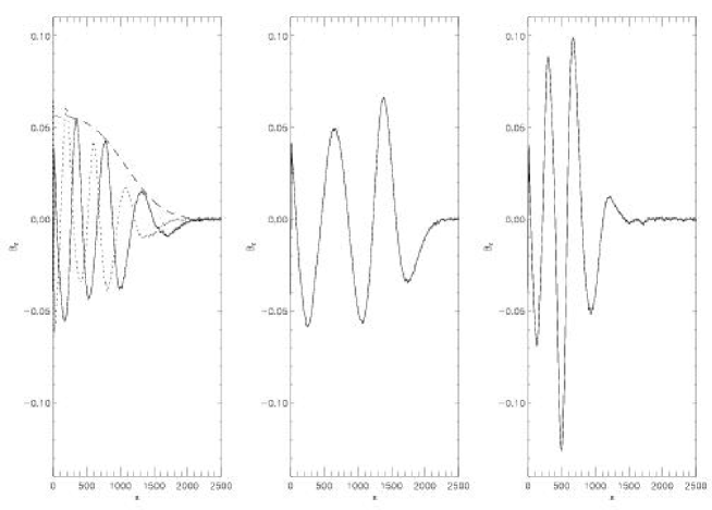
Figure 6: Left: two snapshots of the Alfvén wave $B_{z}(x,y=148)$ component at instances $t=54.69/\omega_{ci}$ (solid line) and $t=46.87/\omega_{ci}$ (dotted line). The dashed line represents fit $0.056\exp\left[-\left({x}/{1250}\right)^{3}\right]$. Center: $B_{z}(x,y=10)$ (low density homogeneous region), $B_{z}(x,y=100)$ (high density homogeneous region). Note the differences in amplitudes and propagation speeds, which are consistent with the equilibrium density and thus Alfvén speed dependence on $y$-coordinate.

In MHD, finite resistivity and Alfvén speed non-uniformity are responsible for the enhanced dissipation via phase mixing. In our PIC simulations (kinetic phase mixing), however, we do not have dissipation and collisions (dissipation). Thus, in our case, wave-particle interactions play the same role as resistivity $\eta$ in the MHD phase mixing (Sagdeev & Galeev 1969). No significant AW dissipation was found away from the density inhomogeneity regions (Fig. 6 middle and right panels, note also the differences in amplitudes and propagation speeds, which are consistent with the imposed density and hence Alfvén speed variation across the $y$-coordinate). This has the same explanation as in the case of MHD – it is in the regions of density of inhomogeneities ($V_{A}^{\prime}\not=0$) that the dissipation is greatly enhanced, while in the regions where $V_{A}^{\prime}=0$ there is no substantial dissipation (apart from the classical $\propto\exp(-\eta x)$ one). In the MHD approximation, the aforementioned amplitude decay law is derived from the diffusion equation, to which MHD equations reduce for large times (developed phase mixing (Tsiklauri et al. 2003)). It seems that the kinetic description leads to the same type of diffusion equation. It is unclear at this stage, however, what physical quantity would play the role of resistivity $\eta$ (from the MHD approximation) in the kinetic regime.

3.1 Homogeneous plasma case

In order to clarify the broadening of the ion velocity distribution function and also for a consistency check we performed an additional simulation in the case of homogeneous plasma. Now the density was fixed at 100 ions/electrons per cell in the entire simulation domain and hence plasma temperature and thermal velocities were fixed too. In such a set up no phase mixing should take place as the AW speed is uniform.

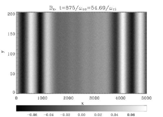
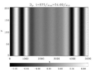
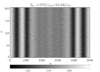
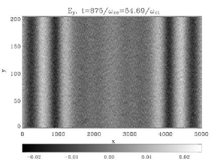
Figure 7: As in Fig. 1 but for the case of homogeneous plasma density (no phase mixing). Note only non-zero (above noise level) components are plotted. There are no $B_{x},E_{x}$ or density fluctuations present in this case.

In Fig. 7 we plot the only non-zero (above noise level) components at $t=54.69/\omega_{ci}$, which are left circularly polarised AW fields: $B_{z},B_{y},E_{z},E_{y}$. Note there are no $B_{x},E_{x}$ or density fluctuations present in this case (cf. Fig. 1) as it is the plasma inhomogeneity that facilitates the coupling between AW and the compressive modes.

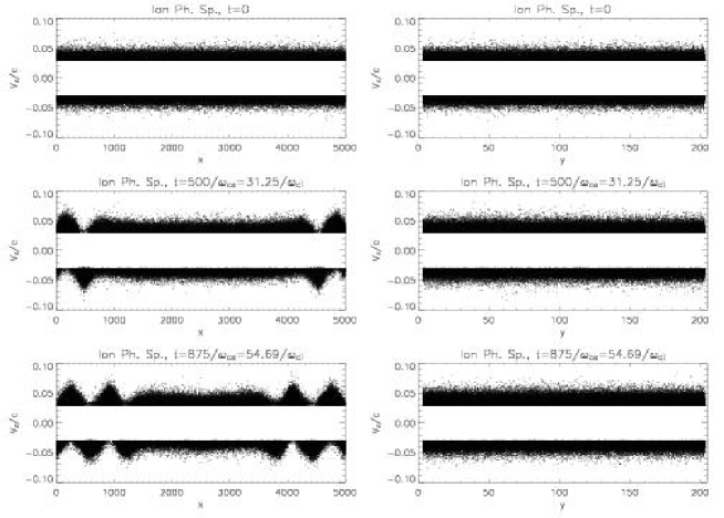
Figure 8: As in Fig. 3 but for the case of homogeneous plasma density (no phase mixing).

In Fig. 8 we plot ion phase space ($V_{z}/c$ vs. $x$ and $V_{z}/c$ vs. $y$) in the homogeneous plasma case for different times (cf. Fig. 3). We gather from the graph that propagating, incompressible, Alfvénic ”kink” type oscillations are still present (left column), while no significant ion acceleration takes place (right column). This is better understood from Fig. 9 where we plot electron and ion distribution functions for $t=0$ and $t=54.69/\omega_{ci}$ (as in Fig. 4) for the homogeneous plasma case. There are three noteworthy points: (i) no electron acceleration takes place because of the absence of phase mixing; (ii) there is (as in the inhomogeneous case) broadening of the ion velocity distribution functions (in $V_{y}$ and $V_{z}$) due to the present AW (wave broadening); (iii) The distribution now looks Maxwellian (cf. Fig. 4) because the distribution function holds for the entire homogeneous region.

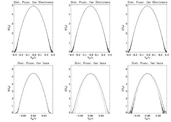
Figure 9: As in Fig. 4 but for the case of homogeneous plasma density (no phase mixing).

In Fig. 10 we plot the kinetic energy $x,y,z$ components ($\propto V_{x,y,z}^{2}$) and total kinetic energy for electrons (top row) and ions (bottom row). For ions we see (as in the inhomogeneous case) that $y$ and $z$ components of the kinetic energy (bottom left figure) oscillate in anti-phase and their oscillatory part perfectly cancels out in the total energy (bottom right figure). Thus, the broadening of the $y$ and $z$ components of the ion velocity distribution functions is due to the presence of AWs, and, in turn, there is no ion acceleration. Again the $y$ and $z$ components and hence the total kinetic energy of the ions is monotonously increasing due to continuous AW driving. No significant motion of ions along the field is present. For electrons we do not observe any acceleration due to the absence of phase mixing (cf. Fig.5). Note that the $y$ component now attains the same values as the $z$ component (bottom left figure) because of the same AW velocity in the entire simulation domain.

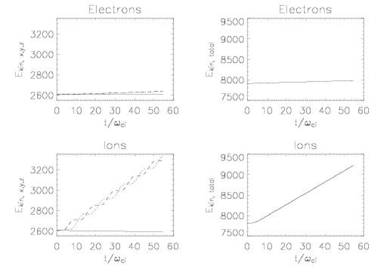
Figure 10: As in Fig. 5 but for the case of homogeneous plasma density (no phase mixing).

4 Discussion

In our preliminary work (Tsiklauri et al. 2005) we outlined the main results of our newly-discovered mechanism of electron acceleration. Here we presented a more detailed analysis of the phenomenon. We have established the following:

• Progressive distortion of the Alfvén wave front, due to the differences in local Alfvén speed, generates oblique (nearly parallel to the magnetic field) electrostatic fields, which accelerate electrons.

• The amplitude decay law in the inhomogeneous regions, in the kinetic regime, is shown to be the same as in the MHD approximation described by Heyvaerts & Priest (1983).

• The density perturbations ($\approx 10$% of background) are generated due to both the weak non-linearity and plasma inhomogeneity. These are propagating density oscillations with variations both in overall magnitude and across the $y$-coordinate. They are mainly confined to the strongest density gradients regions (around $y\approx 50$ and $150$) i.e. edges of the density structure (e.g. boundary of a solar coronal loop). Longitudinal to the external magnetic field, $B_{x}$, perturbations are also generated in the same manner, but with smaller ($\approx 3$%) amplitudes.

• Both in the homogeneous and inhomogeneous cases the presence of AWs causes broadening of the perpendicular (to the external magnetic field) ion velocity distribution functions, while no ion acceleration is observed.

In the MHD approximation Hood et al. (2002) and Tsiklauri et al. (2003) showed that in the case of localised Alfvén pulses, Heyvaerts and Priest’s amplitude decay formula $\propto\exp(-Ax^{3})$ (which is true for harmonic AWs) is replaced by the power law $B_{z}\propto x^{-3/2}$. A natural next step forward would be to check whether in the case of localised Alfvén pulses the same power law holds in the kinetic regime.

After this study was complete we became aware of a study by Vasquez & Hollweg (2004), who used a hybrid code (electrons treated as a neutralising fluid, with ion kinetics retained) as opposed to our (fully kinetic) PIC code, to simulate resonant absorption. They found that a planar (body) Alfvén wave propagating at less than $90^{\circ}$ to a background gradient has field lines which lose wave energy to another set of field lines by cross-field transport. Further, Vasquez (2004) found that when perpendicular scales of the order of 10 proton inertial lengths ($10c/\omega_{pi}$) develop from wave refraction in the vicinity of the resonant field lines, a non-propagating density fluctuation begins to grow to large amplitudes. This saturates by exciting highly oblique, compressive and low-frequency waves which dissipate and heat protons. These processes lead to a faster development of small scales across the magnetic field, i.e. the phase mixing mechanism, studied here.