Adaptive Filters Revisited - RFI Mitigation in Pulsar Observations

Abstract

Pulsar detection and timing experiments are applications where adaptive filters seem eminently suitable tools for radio-frequency-interference (RFI) mitigation. We describe a novel variant which works well in field trials of pulsar observations centred on an observing frequency of 675 MHz, a bandwidth of 64 MHz and with 2-bit sampling. Adaptive filters have generally received bad press for RFI mitigation in radio astronomical observations with their most serious drawback being a spectral echo of the RFI embedded in the filtered signals. Pulsar observations are intrinsically less sensitive to this as they operate in the (pulsar period) time domain. The field trials have allowed us to identify those issues which limit the effectiveness of the adaptive filter. We conclude that adaptive filters can significantly improve pulsar observations in the presence of RFI.

KESTEVEN ET AL. M.KESTEVEN, AUSTRALIA TELSECOPE NATIONAL FACILITY, CSIRO, AUSTRALIA, (michael.kesteven@csiro.au) ADAPTIVE FILTERS FOR PULSAR OBSERVATION

1 Introduction

The days of interference-free observations in radio astronomy are now long gone. Increasingly, observations such as the search for red-shifted HI will need to be made outside the bands allocated to radio astronomy. There are also substantial pressures from commercial, defence and other interests for greater access to the radio-frequency spectrum. This means that the radio astronomers can no longer rely on the regulatory authorities for an interference-free environment; we need to explore the possibilities for co-existence.

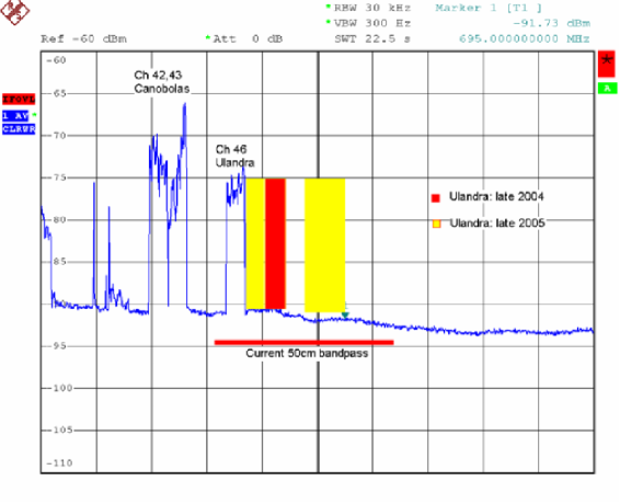
Figure 1: The RFI environment at Parkes in the 50cm band. The frequency span in the image is 200 MHz.

The work described in this paper was prompted by the commissioning of a new digital TV transmitter located on Mt. Ulandra, about 200 km south of the Parkes observatory. This transmitter operates at a frequency of 645 MHz which is within the bandpass of one of the receivers used for pulsar observations. Figure 1 shows the current RFI environment at Parkes at these frequencies and the location of three further transmitters scheduled for commissioning in the near future. While repositioning the receiver bandpass might avoid this particular source of radio-frequency-interference (RFI), it is clear that the observatory needs to continue to develop its expertise in RFI mitigation.

The adaptive filter is one of the promising areas of interference mitigation: the filter detects the presence of interference in the astronomery data, and derives a suitable correction function to remove (or at least reduce) the interference. Several groups at the Australia Telescope National Facility have been engaged in RFI mitigation experiments for a number of years, concentrating in particular on the post-correlation class of adaptive filters (Briggs et al. 2000; Kesteven 2004). This work has been successful in demonstrating useful RFI mitigation in spectroscopy experiments. While the post-correlation adaptive filter may be applicable to pulsar observations, it will be expensive in computational resources.

In this paper, we show that the original form of the adaptive filter is an effective and cost-efficient solution to the requirements of pulsar observations.

2 The Adaptive Filter

Figure 2 summarises the RFI problem to be solved and the nature of the solution. The astronomical antenna collects signals from some target region on the sky. The receiver responds to the astronomical signals primarily from the antenna’s main beam. The antenna also receives interference through one of the many antenna sidelobes. Astronomers will find their data corrupted by this interference – at times to such an extent that the data are useless.

An adaptive filter is a device that can remove much of the interference from the astronomy signal without affecting the astronomical information. The hardware consists of a reference antenna, organised to be very responsive to the interference, and to have little or no response to the astronomy signal. The heart of the device is a filter which acts on the reference antenna signal to modify it into a close copy of the interference in the astronomy channel. A subtraction will then yield a cleaned astronomy signal that is free of interference. The third component of the adaptive filter is a mechanism to control the filter in order to meet some optimising criterion. Such a device, based on a convolutional filter, was described in detail by Barnbaum & Bradley (1998). It is an elegant scheme which operates directly on the intermediate frequency band (IF) that the astronomer would direct to final processing stage – the pulsar de-dispersing, folding and timing computer in our case.

Assume, for the moment, that the system is operating in a narrow radio frequency band. In this case, we would require the filter to adjust the gain and phase of the reference IF until the interference is a good match to the interference in the astronomical channel. A subtraction will yield an interference-free IF. Unfortunately the reference IF also contains noise from its receiver. Increasing the gain in order to balance the RFI will allow an increasing amount of receiver noise into the output IF. Decreasing the gain degrades the interference cancellation. Since the astronomer generally does not distinguish noise power from interference power in his spectrum, the optimum filter gain (from the astronomer’s perspective) is the setting with the minimum additional power in the output IF.

More formally, let:

$$P_{out}=N_{ast}+P_{rfi}\times(c_{ast}-g*c_{ref})^{2}+g^{2}N_{ref}$$

where $N$ is the receiver noise power in the astronomy ($ast$) or reference ($ref$) channels, $P_{rfi}$ is the interference power at the site, $c$ describes the complex voltage coupling of the interference into the two channels and $g$ is the complex voltage gain of the filter.

Minimising $P_{out}$ with respect to g leads to :

$$g=\frac{c^{*}_{ast}c_{ref}P_{rfi}}{N_{ref}+c^{2}_{ref}P_{rfi}}$$

The power at this optimal gain setting is:

$$P_{out}=N_{ast}+\frac{c^{2}_{ast}P_{rfi}}{(1+{\rm INR})}$$

where INR is the ratio of the interference power in the reference IF to the noise power,

$${\rm INR}=\frac{c^{2}_{ref}P_{rfi}}{N_{ref}}$$

In other words, the astronomer will see the “interference” in his spectrum reduced from P (= $c^{2}_{ref}P_{rfi}$) to P/(1 + INR). With no filtering the spectrum is corrupted by interference; with the filter in operation the corruption is due to a small residue of interference along with a small fraction of noise from the receiver in the reference channel.

The adaptive filter in practice operates over a wide frequency range. The scheme outlined above is readily modified to suit that need by recognising that the gain is frequency dependent and implementing the filter as a convolutional filter. The cross-spectrum output from the correlator is then the Fourier transform of the correction to the filter weights. The filter weights are optimised when the cross-spectrum is zero.

The correlator output will of course be subject to noise fluctuations which can be smoothed by averaging. The appropriate averaging time is set by the time scale on which the noise-free filter settings would change, i.e. by the time scale on which the coupling terms change. This is set by propagation considerations such as the relative delay between the reference and astronomy antennas, or the changing proportions of the multi-path propagation. As these are relatively slow effects, we used in the pulsar experiments a time scale of 3 ms.

The FIR weights are computed as follows. Let $\{w^{n}_{i}\}$ be the set of weights in use during the n-th integration, R(t) is the voltage in the reference channel, A(t) the voltage in the astronomical channel and F(t) is the voltage output from the FIR filter,

$$F_{j}=\sum_{i}R_{(j-i)}w^{n}_{i}$$

The cross-correlation terms can be written as

$$C_{i}=\frac{1}{N}\sum_{k}(A_{k}-F_{k})R_{(k-i)}$$

and the updated weights are

$$w^{n+1}_{i}=w^{n}_{i}+\epsilon C_{i}$$

where $\epsilon$ controls the convergence of the filter to the optimum setting. The loop is critically damped when $\epsilon=1/Tsys_{ref}$.

This filter has a number of desirable qualities:

1. It adapts automatically to changes in the coupling coefficients. This is important as different sidelobes could be involved as the antenna follows a source. The relative delay between the reference and astronomical antennas may change if the interference source is moving (e.g., a satellite). It will accomodate to changes in the receiver gains.

2. The filter is robust to multi-path propagation.

3. The filter action ceases when the interference ceases. There is no noise penalty at low to zero interference.

4. It can handle multiple independent sources of interference provided that there is no overlap in frequency.

5. Filters can be cascaded which would allow the system to accommodate sources which overlap in frequency. This strategy is also relevant if the interference is so spread out in direction that multiple reference antennas are required.

To the astronomer’s eye, the filter reduces the interference-related noise power by an attenuation factor equal to 1/(1+INR). The filter starts to become ineffective when INR $\sim$ 1.

3 The Field Trials

The Parkes observatory has an on-line pulsar processor (known as CPSR2) that was constructed by the Caltech and Swinburne University groups (Bailes, 2003). This unit streams two baseband IFs (two polarisations, each IF sampled at 128 MSamples/sec), each 64 MHz wide to a disk farm, for real-time processing by a bank of 32 PCs. Each PC is assigned a 1-GByte file for dedispersing, folding at the pulsar period and timing. Our long-term aim is to build a hardware adaptive filter and install it ahead of the processor and other data acquistion systems.

For the current experiments we exploit the CPSR2 architecture to develop the interference rejection algorithm and explore the practical difficulties in RFI mitigation with the use of a software filter. The schemes are shown in figure 3. The software filter cannot support real-time operation, but in every other respect it provides a comprehensive trial. We take two disk files, one with dual-polarisation pulsar data, the second with the IF from the reference antenna and we adaptively filter the pulsar data to create a fresh file with filtered data. This file is inserted back into the system for standard processing.

The reference antenna is mounted on the tallest tower at the observatory and has been oriented to maximise the signal received from Mt. Ulandra. The original experiments used a yagi antenna; this has since been replaced by a 3.5m diameter antenna. The astronomical targets are a variety of pulsars that are detectable in a 16-sec observation. Most of the results shown below are based on the millisecond pulsar PSR J0437$-$4715 which has a period of 5.7 ms. The observing band centre is set to 675 MHz, the bandwidth to 64 MHz and we use 2-bit sampling.

The observations can address the following questions:

1. Does our filter implementation behave as predicted?

2. Does our filter introduce pulsar specific side-effects?

3. Are there other factors which limit the effectiveness of the filter in mitigating the RFI?

4. Are there specific sampling issues that need to be addressed?

3.1 Filter Performance

We have implemented in software the filter shown in figure 2. Although the data is 2-bit sampled, all the operations within the filter are 32-bit floating. The output is normalised and resampled to 8-bits to provide data in a format suitable for the down-stream processing.

The FIR filter has 128 taps (the number of delay steps in the filter), as does the cross-correlator. The spectral resolution is a sin(x)/x window of width 1 MHz, set by the sampling rate (128 MS/s) and the number of taps. The FIR weights are revised every 3 ms. The weights will need to be updated if there are changes in the way the interference appears in the reference and astronomy IFs. For example, while the main antenna is following a sidereal target its sidelobes will track over the source of interference. The interference may also suffer multipath propagation to the reference antenna leading to episodes of fading. Our experiments suggest that at our site the characteristic timescale for these effects (see figure 5) is measured in seconds.

Figure 4 provides an overall picture of the filter’s performance. It shows the IF power spectra before and after filtering. The INR is large and the residual noise (the difference between the filtered spectrum and the RFI-free receiver bandpass) is low, consistent with the large INR in the reference channel.

Figure 5 presents a different perspective. The filter is analysed at 3 ms integrations during the processing. This example was selected to highlight a problem: during the 16 second observation the RFI amplitude changed in both the reference and astronomy channels independently. We believe that this is due to multipath propagation acting independently on the astronomy and reference channels. The 3 ms update interval is adequate to follow these changes, and the attenuation tracks the INR as predicted.

Our observations all indicate that the filter behaves as predicted, with a clear message that maintaining a large INR is vital.

3.2 Are there Side-Effects?

Our brief is to ensure that the filter does not affect the spectral, polarisation or timing characteristics of the pulsar. Our approach has been to do detailed comparisons of the processed data – with and without filtering.

Figures 6 and 7 show the typical raw material, the output from the pulsar processor with data folded at the pulsar period. There are 2048 channels along the pulsar phase axis and 128 along the frequency axis. The data has been de-dispersed, so the pulsar’s “pulse” is visible as the vertical trace near pulsar phase 0.5. The basic question is whether the pulse in the RFI spectral channels has the same characteristics as the pulse in the RFI-free channels.

Figure 8 provides an analysis of the data in figures 6 and 7. These figures show the detected power, after folding and de-dispersing, as a function of pulsar phase and observing frequency ($P(\phi,f)$). Each column in figure 8 has four plots. The first plot shows the power spectra ($\int P(\phi,f)d\phi$) and the second plot shows the pulsar amplitude ($\int P(\phi,f)df$). The effect of the RFI in the unfiltered is evident in increased noise throughout the pulsar phase. The third plot shows the pulse peak amplitude as a function of frequency to show the RFI effect in more detail ($\int^{0.55}_{0.45}P(\phi,f)d\phi$). The full impact of the RFI is shown in the fourth plot, the signal-to-noise ratio in the peak amplitude.

Outside the RFI range the filtered and unfiltered data are identical (to within the re-sampling error). In the RFI range the filtered data are consistent with interpolations from the adjacent channels. For these observations the reference signal was obtained from the 3.5m antenna.

3.3 Additional RFI Mitigation Problems

At this stage in our investigations we conclude that the adaptive filter could provide a solution to the RFI mitigation question provided that we can master the apparently random and uncorrelated power variations in the RFI that are shown in figure 5.

We suggest that the underlying mechanism is multipath propagation which leads to destructive interference. We are exploring a number of counter-measures:

• Installing a larger antenna which could raise the signal power and reduce the number of multi-path rays.

• Installing a second reference antenna displaced from the first to provide some spatial diversity. We would need to add an intelligent IF switch to select the better of the two filtered IFs.

• Exploiting the known coding algorithm of the digital TV to reconstruct a better reference signal with higher (and stable) INR. A variant of this strategy has been demonstrated as way to mitigate GLONASS RFI by Ellingson et al. (2001).

3.4 Sampling Issues

Two-bit sampling has not been a limitation to these experiments. Even though the RFI is substantially larger than the receiver noise, it is confined to about 10% of the receiver bandpass and does not dominate the noise presented to the sampler. We suffer a further penalty in the resampling stage at the filter output. However, the present experiment suggests that such loss is modest. Care is also required in the resampling stage since the filtered data may retain echoes of the original two-bit sampling; a poor setting of the thresholds can negate much of the filter’s action.

As pulsar observers lock the sampler thresholds during an observation, non-stationarity might seem to be an additional potential source of trouble. However, the adaptive filter should be neutral to this provided that the relation between measured and true correlation coefficients remains linear. See Jenet and Andersen (1998) for a detailed discussion of this issue.

4 Conclusion

The results of this program are encouraging - we believe that the adaptive filter will be able to provide a satisfactory level of RFI mitigation. We will shortly move to a hardware implementation of the filter.

It is clear that the mitigation can only succeed if we have a high quality copy of the interference; we will need to devote more time and effort into this side of the problem in the coming months.

Figure 2: The pre-detection filter. We require a reference antenna which captures a copy of the interference while remaining insensitive to the astronomical signal. The filter modifies the reference antenna’s signal into a close copy of the interference in the astronomy signal.

Figure 3: The pulsar processing models. The top figure shows the current implementation. The middle figure shows our long term aim: a real-time hardware filter which cleans the IF ahead of the CPSR2 processor. The lower figure shows our development mode: a software filter operates on a file of data, replacing it with a filtered version for subsequent processing. In this mode the operation is not real time.

Figure 4: The filter in action. The top panel shows the raw astronomy IF, the middle panel shows the reference IF (INR $\sim$ 50:1) and the lower panel shows the filtered IF.

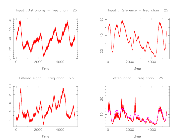
Figure 5: The filter in action. Each plot shows the filter performance in one selected frequency channel (number 25), computed every 3 ms. The plot at the lower right shows the attenuation (filtered excess noise power divided by the excess noise in the raw astronomy IF, where “excess noise power” is the amplitude above the RFI-free level). The attenuation computed from the INR of the reference IF is also shown - it is the trace which is essentially free of noise.

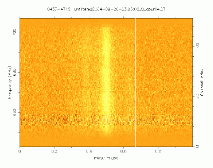
Figure 6: The output from the pulsar processor after de-dispersion and folding at the pulsar period of a 16.7-sec segment of unfiltered data.

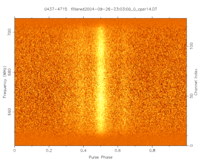
Figure 7: The output from the pulsar processor after de-dispersion and folding at the pulsar period of filtered data.

Figure 8: A statistical summary of figures 6 and 7. The top panel shows the mean power in each frequency channel. The second panel shows the pulse profile. The third panel shows the amplitude of the pulsar pulse, at each frequency; it is the power summed over a narrow window in pulsar phase centred on the pulse peak. The fourth panel shows the Signal-to-Noise ratio of the pulse amplitude.

- [1] Bailes, M Radio Pulsars ASP Conference series CS-302, 57, 2003.
- [2] Barnbaum, C. and Bradley, R.F. A.J. 115, 2598, 1998.
- [3] Briggs, F., Bell, J. and Kesteven, M. A.J. 120, 3351, 2000.
- [4] Ellingson, S.W., Bunton, J.D. and Bell, J.F. Ap.J.Suppl. 135, 87, 2001
- [5] Jenet, F.A., Andersen, S.R. PASP, 110, 1467, 1998.
- [6] Kesteven, M New Technologies in VLBI, nov. 2002, Gyeong-Yu, Korea. ASP Conference series CS-307, 93, 2003.