8000

2001

The mass-metallicity relation at $z\sim 0.7$

Abstract

The ISM metallicity and the stellar mass are examined in a sample of 66 galaxies at $0.4<z<1$, selected from the Gemini Deep Deep Survey (GDDS) and the Canada-France Redshift Survey (CFRS). We observe a mass-metallicity relation similar to that seen in $z\sim 0.1$ SDSS galaxies, but displaced towards higher masses and/or lower metallicities. Using this sample, and a small sample of $z\sim 2.3$ LBGs, a redshift dependent mass-metallicity relation is proposed which describes the observed results.

0.1 Introduction

The mass and the metallicity of galaxies are important physical parameters which are exhaustedly studied in the local Universe. At low redshift ($z\sim 0.1$) a convincing correlation between the stellar mass and the metallicity in the ISM was found in a sample of 53,000 SDSS star-forming galaxies (Tremonti et al. 2004). At higher redshift, this test was never attempted, due to the difficulty to obtain mass (which requires NIR photometry) together with metallicity (which requires optical/NIR spectroscopy) for a large sample of faint objects. As an alternative parameter for mass, the galaxy optical luminosity can be used, although this is affected by dust extinction. At $0.3<z<1$, Kobulnicky & Kewley (2004) found a correlation between luminosity and mass, with an offset towards higher luminosities with respect to the SDSS sample, suggesting a time evolution of the luminosity-metallicity relation. Low metallicities (for the observed luminosities) are also detected in some LBGs at $z\sim 2.3$ (Shapley et al. 2004). In this work we present the first investigation of the mass-metallicity relation at high redshift.

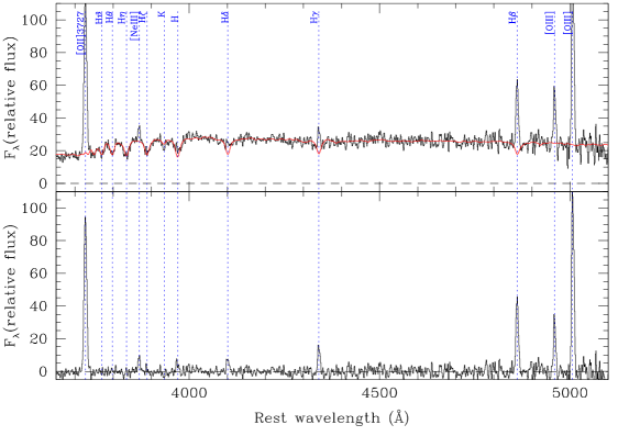
Figure 1: Composite spectrum of 26 GDDS galaxies in $0.47<z<0.96$ (upper panel), with overplotted the “best-fit” stellar population model (Bruzual & Charlot 2003). The lower panel shows the emission lines after the stellar continuum subtraction. The equivalent width Balmer absorption correction is of the order of 3 Å both for H$\beta$ and H$\gamma$, depending on the emission line FWHM.

0.2 The sample and the composite spectrum

The sample selection from the GDDS (Abraham et al. 2004) is based on the requirement that the spectra wavelength interval covers the [OII], [OIII] and H$\beta$ emission lines (30 galaxies in $0.4<z<1.00$). To measure emission line fluxes, the continuum was estimated from two small regions before and after the line. In those cases where the [OIII]$\lambda 4958$ emission line is barely detected, the flux is assumed to be 0.34 times lower than the [OIII]$\lambda 5007$ line flux (as set by atomic parameters).

The stellar Balmer absorption correction in the individual spectra is done by using the mean Balmer absorption in the composite spectrum. This is estimated by fitting the stellar continuum with Bruzual & Charlot (2003) stellar population synthesis models. The composite spectrum is also used to derive the dust extinction, via the Balmer decrement measurement, which gives an optical extinction $A_{V}=2.2\pm 0.3$ (for a gas temperature $T=10,000$ K, and a Milky Way extinction law). For 1/3 of the galaxies, the H$\gamma$ emission line is detected, and the Balmer decrement estimated directly.

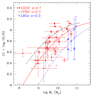
Figure 2: Left panel: Mass vs. metallicity for $z\sim 0.7$ galaxies in the GDDS (filled squares: $K<20.6$; filled triangles: $K>20.6$) and CFRS (open squares), and for $2.1<z<2.4$ LBGs (crosses). LBG metallicities are taken from Shapley et al. (2004) after a correction in mass and metallicity which takes into account the different IMF and metallicity calibrator used. The left long-dashed curve is the best fit polynomial fit to 53,000 SDSS $z\sim 0.1$ galaxies (Tremonti et al. 2004). The solid and short-dashed lines are the same curve shifted to the right to match the GDDS+CFRS and LBG distributions. Right panel: The shift in mass applied to the SDSS mass-metallicity relation to match the GDDS+CFRS and LBG distributions. Error bars indicate the $\sim 1\sigma$ mass dispersion around the mass-metallicity relation in the three samples.

0.3 The Mass-Metallicity Relation at $z\sim 0.7$

Dust extinction and Balmer absorption corrected emission line fluxes in the GDDS galaxies were used to estimate ISM metallicities via the $R_{23}$ parameter (Pagel et al. 1979). The particular metallicity:$R_{23}$ relation used is the one recently provided by Kobulnicky & Kewley (2004). Metallicities for the CFRS sample are those derived by Lilly et al. (2003), after a small correction of $+0.06\ dex$ to account for the different metallicity:$R_{23}$ relation used. Stellar masses of GDDS and CFRS galaxies are derived when the $K$ or $z^{\prime}$ band magnitudes are measured, using the method described in Glazebrook et al. (2004). The left panel of Figure 2 shows metallicities vs. mass for the total sample of 25+41 galaxies. The low redshift mass-metallicity relation of the SDSS galaxies is shown as a long-dashed line, and the same relation displaced to the right by $\Delta\log M_{\star}=0.54$ as a solid line. This displacement is interpreted as due to a redshift evolution of the mass-metallicity relation: galaxies at high redshift tend to have higher masses (or lower metallicities) with respect to galaxies with the same metallicities (or same masses) in the local Universe. This conclusion is not disproved by the results for 7 LBGs at $z\sim 2.3$ (Shapley et al. 2004), which have, for the measure metallicities, higher stellar masses (crosses in the left panel of Figure 2). Note that LBGs have been shifted to higher metallicities and lower masses, to correct for the different metallicity calibrator and IMF used. The right panel of Figure 2 shows the displacements in mass in the mass-metallicity relation as a function of the age of the Universe, for the three samples at redshifts $z\sim 0.1,0.7$ and 2.3.

Tremonti et al. (2004) provide a mass-metallicity polynomial fit of the form:

$$12+\log{\rm(O/H)}=-1.492+1.874y-0.08026y^{2}$$ (1)

where $y\equiv\log M_{\star}$. If we use the fit in the right panel of Figure 2, the parameter $y$ can be expressed by:

$$y=\log M_{\star}+2.003\log t_{H}-2.194$$ (2)

and Eqs. 1 and 2 give a general mass-metallicity relation that is also function of the Hubble time $t_{H}$ (expressed in Gyr). These two relations together are shown in Figure 3, where metallicity is displayed as a function of the stellar mass (for fixed redshifts, left panel) or as a function of the Hubble time (for fixed stellar masses, right panel).

This empirical model, which describes the joint redshift evolution of the stellar mass and metallicities, is a very exciting result that is certainly opening a new view towards the cosmic metal production, both from the theoretical and the observational point of view. A galaxy sample in a restricted mass interval, can only provide a partial understanding of this problem. In the near future we will adopt simple theoretical methods, which use different approaches for the IMF and SN feedback, to model mass and metallicity of galaxies from their birth to the present.

Figure 3: Metallicity as a function of stellar mass, for constant redshifts (left panel) or as a function of Hubble time for constant stellar masses (right panel). These relations are obtained by extrapolating at higher redshifts the Tremonti et al.’s relation (obtained for the SDSS galaxies).

References

- (1) Abraham et al. 2004, AJ, 127, 2455
- (2) Glazebrook, K., et al. 2004, Nature, 430, 181
- (3) Kobulnicky, H. A., & Kewley L. J. ApJ, 2004, in press
- (4) Lilly, S. J., Carollo, C. M., & Stockton, A. N. 2003, ApJ, 597, 730
- (5) Shapley, A. E., Erb, D. K., Pettini, M., Steidel, C. C., Adelberger K. L. 2004, ApJ, 612, 108
- (6) Tremonti, C. A., et al. 2004, ApJ, 613, 898