On detecting terrestrial planets with timing of giant planet transits

Abstract

The transits of a planet on a Keplerian orbit occur at time intervals exactly equal to the period of the orbit. If a second planet is introduced the orbit is not Keplerian and the transits are no longer exactly periodic. We compute the magnitude of these variations in the timing of the transits, $\delta t$. We investigate analytically several limiting cases: (i) interior perturbing planets with much smaller periods; (ii) exterior perturbing planets on eccentric orbits with much larger periods; (iii) both planets on circular orbits with arbitrary period ratio but not in resonance; and (iv) planets on initially circular orbits locked in resonance. Using subscript “out” and “in” for the exterior and interior planets, $\mu$ for planet to star mass ratio and the standard notation for orbital elements, our findings in these cases are as follows: (i) Planet-planet perturbations are negligible. The main effect is the wobble of the star due to the inner planet, therefore $\delta t\sim\mu_{in}(a_{in}/a_{out})P_{out}$. (ii) The exterior planet changes the period of the interior one by $\mu_{out}(a_{in}/r_{out})^{3}P_{in}$. As the distance of the exterior planet changes due to its eccentricity, the inner planet’s period changes. Deviations in its transit timing accumulates over the period of the outer planet, therefore $\delta t\sim\mu_{out}e_{out}(a_{out}/a_{in})^{3}P_{out}$. (iii) Half way between resonances the perturbations are small, of order $\mu_{out}a_{in}^{2}/(a_{in}-a_{out})^{2}P_{in}$ for the inner planet (switch “out” and “in” for the outer planet). This increases as one gets closer to a resonance. (iv) This is perhaps the most interesting case since some systems are known to be in resonances and the perturbations are the largest. As long as the perturber is more massive than the transiting planet, the timing variations would be of order of the period regardless of the perturber mass! For lighter perturbers, we show that the timing variations are smaller than the period by the perturber to transiting planet mass ratio. An earth mass planet in 2:1 resonance with a 3-day period transiting planet (e.g. HD 209458b) would cause timing variations of order 3 minutes, which would be accumulated over a year. These are easily detectable with current ground-based measurements.

For the case of both planets on eccentric orbits, we compute numerically the transit timing variations for several cases of known multiplanet systems assuming they were edge-on. Transit timing measurements may be used to constrain the masses and radii of the planetary system and, when combined with radial velocity measurements, to break the degeneracy between mass and radius of the host star.

1 Introduction

The recent discovery of planets orbiting other stars (“exoplanets”) has opened a new field of astronomy with the potential to address fundamental questions about our own solar system which we can now compare with other planetary systems. The primary mode for discovery of exoplanets has been the measurement of the stellar radial velocities via the Doppler effect. Currently the small reflex motion of the star due to the orbiting planet can only be detected for $m_{planet}\ga 10m_{\oplus}$ (Butler et al., 2004; McArthur et al., 2004; Santos et al., 2004). More recently, a large number of planetary transit searches are being carried out which are starting to yield an handful of giant planets (Charbonneau et al., 2000; Konacki et al., 2003; Pont et al., 2004; Konacki et al., 2004; Bouchy et al., 2004; Alonso et al., 2004), and many more planned searches should reap a large harvest of transiting planets in the near future (Horne, 2003). Despite these successes, the discovery of “terrestrial” exoplanets, similar in size to the earth, awaits the development of several other techniques such as astrometry, space-based transit searches, microlensing, or direct imaging (Perryman, 2000; Charbonneau, 2003; Ford & Tremaine, 2003; Borucki et al., 2003; Gould et al., 2004).

The first transiting planetary system, HD 209458b, was discovered with Doppler motions of the primary star (Charbonneau et al., 2000). Since the mass of the planet is degenerate with orbital inclination, the planetary status of the companion was confirmed since the transits imply it is edge-on. HST observations yielded precision measurements of the transit lightcurve (Brown et al., 2001), which made this the surest planetary candidate around a main sequence star (other than our own). The ratio of the planetary radius to the stellar radius can be measured with extreme precision (Mandel & Agol, 2002). However, the absolute radii are uncertain due to a degeneracy between radius and mass of star (Seager & Mallén-Ornelas, 2003): an increase in the mass and radius of the star can yield an identical lightcurve and period.

This mass-radius degeneracy may be broken if there is an additional planet in the system. About 10 per cent of the stars with known planetary companions have more than one planet, while possibly as much as 50 per cent of them show a trend in radial velocity indicative of additional planets (Fischer et al., 2001). If one or both of the planets is transiting, dynamical interactions between the planets will alter the timing of the transits (Dobrovolskis & Borucki, 1996; Charbonneau et al., 2000; Miralda-Escudé, 2002). A measurement of these timing variations, combined with radial velocity data, can break the mass-radius degeneracy.

Given the dual motivations of detecting terrestrial planets and breaking the mass-radius degeneracy, we derive analytic and numerical results for transit timing variations due to the presence of a second planet. We begin our discussion by introducing the three-body system in §2. The signal from non-interacting planets is calculated first (§3) and then we compute the effects of an eccentric exterior perturbing planet with a large period in §4. A derivation of the general transit timing differences for two planets with circular, co-planar orbits is presented in §5. The case of exact mean-motion resonance is analyzed in §6. The case of two eccentric planets is considered in §7, along with numerical simulations of several known multi-planet systems (these are not transiting). We show how measurements of the dispersion of transit timings can be used to detect a secondary planet in the system (§8.1), we compare to other planet-search techniques (§8.2), and we show how to determine the absolute size and mass of the objects in the system (§8.3). Finally, we discuss other effects we have ignored that an observer should be conscious of (§9).

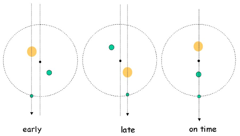
Figure 1: Cartoon showing changes in the timing of transit due to a perturbing planet interior to the orbit of a transiting planet.

Throughout the rest of the paper we characterize the strength of transit timing variations as follows. For a series of transit times, $t_{j}$, we fit the times assuming a constant period, $P$. We compute the standard deviation, $\sigma$, of the difference between the nominal and actual times. Mathematically,

$$\sigma={1\over N}\left[\sum_{j=0}^{N-1}(t_{j}-t_{0}+Pj)^{2}\right]^{1/2},$$ (1)

where $P$ and $t_{0}$ are chosen to minimize $\sigma$. If the variations are strictly periodic, then the amplitude of the timing deviation is simply $\sqrt{2}$ times larger than $\sigma$.

During the preparation of this paper a proceedings contribution has appeared by Jean Schneider which considers several of the effects discussed here (Schneider, 2003); however, we find that Schneider’s results are incorrect as he does not consider the differential force between the star and the transiting planet. In addition, calculations similar to those presented here are being carried out by Matt Holman and Norm Murray.

2 Equations of Motion

We are studying the 3-body system in which the three bodies have labels $0,1,2$ and positions ${\bf R}_{i},i=0,1,2$ (with an arbitrary origin). The exact Newtonian equations of motion are given by

$$\ddot{\bf R}_{i}=\sum_{j\neq i}Gm_{j}{{\bf R}_{j}-{\bf R}_{i}\over|{\bf R}_{j}-{\bf R}_{i}|^{3}}.$$ (2)

Multiplying the equations for each particle by its mass and adding together, one finds:

$$m_{0}\ddot{\bf R}_{0}+m_{1}\ddot{\bf R}_{1}+m_{2}\ddot{\bf R}_{2}=0.$$ (3)

This is simply a statement that the centre of mass of the system has no external forces. Since light travel time and parallax effects are negligible (§9.1), the transit problem is unaffected by the total velocity or position of the centre of mass, so we set

$${\bf R}_{cm}\equiv{\sum_{i=0}^{2}m_{i}{\bf R}_{i}\over\sum_{i=0}^{2}m_{i}}=0.$$ (4)

This reduces the differential equations of motion to two, which we take to be that of the two planets, $R_{1}$ and $R_{2}$ (for the two planetary masses). We use this system of equations for numerically solving the equations of motion. However, for analytic consideration it is more convenient to write the problem in Jacobian coordinates which we discuss next.

The Jacobian coordinate system is commonly used in perturbation theory for many bodies (see, e.g. Murray & Dermott, 1999; Malhotra, 1993a, b). For the three-body problem, the Jacobian coordinates amount to three new coordinates which describe (a) the centre of mass of the system; (b) the relative position of inner planet and the star (the “inner binary”); (c) the relative position of the outer planet and the barycentre of the inner binary (the “outer binary”). To distinguish from the body coordinates, we denote the Jacobian coordinates with a lower case ${\bf r}_{i}$. The Jacobian coordinates are

$${\bf r}_{0} = {\bf R}_{cm}=0,$$ (5)

$${\bf r}_{1} = {\bf R}_{1}-{\bf R}_{0},$$ (6)

$${\bf r}_{2} = {\bf R}_{2}-{1\over m_{0}+m_{1}}\left[m_{0}{\bf R}_{0}+m_{1}{\bf R}_{1}\right].$$ (7)

Using $\mu_{i}=m_{i}/M\sim m_{i}/m_{0}$, where $M=\sum_{i=0}^{2}m_{i}$, the equations of motion may be rewritten in Jacobian coordinates,

$$\ddot{{\bf r}}_{1} = -{Gm_{0}\over 1-\mu_{1}}{{\bf r}_{1}\over r_{1}^{3}}-GM\mu_{2}{{\bf r}_{1}-{\bf r}_{21}\over|{\bf r}_{1}-{\bf r}_{21}|^{3}}-GM\mu_{2}{{\bf r}_{21}\over r_{21}^{3}},$$ (8)

$$\ddot{{\bf r}}_{2} = -{Gm_{0}\over 1-\mu_{2}}{{\bf r}_{21}\over r_{21}^{3}}-GM\mu_{1}{{\bf r}_{21}-{\bf r}_{1}\over|{\bf r}_{21}-{\bf r}_{1}|^{3}},$$ (9)

where ${\bf r}_{21}=\mu_{1}{\bf r}_{1}+{\bf r}_{2}={\bf R}_{2}-{\bf R}_{0}$.

3 Non-interacting planets: Perturbations due to interior planet on a small orbit

Throughout the rest of the paper we make the approximations that (a) the orbits of both planets are aligned in the same plane; (b) the system is exactly edge-on, that is, the inclination angle is 90^∘. We also approximate the planet and star as spherical so that the transit is symmetric with a well-defined midpoint.

If we take the limit as $\mu_{1},\mu_{2}\rightarrow 0$ in equation (8), then the orbits of the planets follow Keplerian trajectories with the equations of motion

$$\ddot{{\bf r}}_{1} = -Gm_{0}{{\bf r}_{1}\over r_{1}^{3}},$$ (10)

$$\ddot{{\bf r}}_{2} = -Gm_{0}{{\bf r}_{2}\over r_{2}^{3}}.$$ (11)

This approximation requires that the periapse of the outer planet be much larger than the apoapse of the inner planet, $(1-e_{2})a_{2}\gg(1+e_{1})a_{1}$ where $a_{1},a_{2}$ are the semi-major axes of the inner and outer binary and $e_{1},e_{2}$ are the eccentricities. In this case, the inner binary orbits about its barycentre which in turn orbits about the barycentre of the outer binary but there is no perturbation to the relative motion of the inner binary due to gravitational interactions. Timing variations that arise are simply due to the reflex motion of the star (as shown in Figure 1).

The simplest case to consider is that in which both the inner and outer binary are on approximately circular orbits. The transit occurs when the outer planet is nearly aligned with the barycentre of the inner binary and its motion during the transit is essentially transverse to the line of sight. The inner planet displaces the star from the barycentre of the inner binary by an amount

$$x_{0}=-a_{1}\mu_{1}\sin{\left[2\pi(t-t_{0})/P_{1}\right]},$$ (12)

where the inner binary undergoes a transit at time $t_{0}$ and $P_{1}$ is the orbital period of the inner binary. Thus, the timing deviation of the $m$th transit of the outer planet is

$$\delta t_{2}\approx-{x_{0}\over v_{2}-v_{0}}\approx-{P_{2}a_{1}\mu_{1}\sin{\left[2\pi(mP_{2}-t_{0})/P_{1}\right]}\over 2\pi a_{2}},$$ (13)

where $v_{i}$ is the velocity of the $i$th body with respect to the line of sight. Typically $v_{0}\ll v_{2}$, so we have neglected $v_{0}$ in the second expression in the previous equation.

Computing the standard deviation of timing variations over many orbits gives

$$\sigma_{2}=\langle(\delta t_{2})^{2}\rangle^{1/2}={P_{2}a_{1}\mu_{1}\over 2^{3/2}\pi a_{2}}.$$ (14)

Note that if the periods have a ratio $P_{2}$:$P_{1}$ of the form $q$:$1$ for some integer $q$, then the perturbations disappear since the argument of the sine function is the same each orbit. Another observable is the duration of the transit, which scales as

$$t_{2}\approx{2R_{*}\over(v_{2}-v_{0})}.$$ (15)

This leads to significant variations only if $v_{0}\simeq v_{2}$, or $\mu_{1}^{2}>a_{1}/a_{2}$, which requires a very large axis ratio.

More interesting variations occur if either or both planets are on eccentric orbits. Because both planets are following approximately Keplerian orbits, the transit timing variations and duration variations can be computed by solving the Kepler problem for each Jacobian coordinate. Since we are assuming that the planets are coplanar and edge-on, 4 coordinates each suffice to determine the planetary positions: $e_{1,2}$, $a_{1,2}$, $\varpi_{1,2}$ (longitude of pericentre), and $f_{1,2}$ (true anomaly). As in the circular case, the change in the transit timing is approximately $\delta t_{2}\approx{x_{0}/v_{2}}$. The position of the star with respect to the barycentre of the inner binary is

$$x_{0}=-\mu_{1}r_{1}\sin{\left[f_{1}+\varpi_{1}\right]}.$$ (16)

If $a_{1}\ll a_{2}$, the outer planet is in nearly the same position at the time of each transit and its velocity perpendicular to the line of sight is

$$v_{2}={2\pi a_{2}\left(1+e_{2}\cos{\varpi_{2}}\right)\over P_{2}\sqrt{1-e_{2}^{2}}},$$ (17)

where we have used the fact that $f_{2}=-\varpi_{2}$ at the timing of the transit. Thus, to first order in $a_{1}/a_{2}$

$$\delta t_{2}=-{P_{2}\mu_{1}r_{1}\sin{[f_{1}+\varpi_{1}]}\sqrt{1-e_{2}^{2}}\over 2\pi a_{2}(1+e_{2}\cos{\varpi_{2}})}.$$ (18)

The standard deviation of $\delta t_{2}$ can be computed analytically as well. Over many transits by the outer planet, the inner binary’s position populates all of its orbit provided the planets do not have a period ratio that is the ratio of two integers. Consequently, we find the mean transit deviation by averaging over the probability that the inner binary is at any position in its orbit, $p(f_{1})=n_{1}/\dot{f}_{1}$ (where $n_{1}=2\pi/P_{1}$), times the transit deviation at that point. This gives

$$\langle\delta t_{2}\rangle = {1\over 2\pi}\int_{0}^{2\pi}df_{1}\delta t_{2}p(f_{1})$$ (19)

$$= -{3\over 2}\mu_{1}{a_{1}\over v_{2}}e_{1}\sin{\varpi_{1}}.$$ (20)

Since the star spends more time near apoapse, the mean timing grows as $e_{1}$. The symmetry of the orbit about $\varpi=0$ and $\pi$ explains the dependence on $\sin{\varpi_{1}}$. A similar calculation gives $\langle\delta t_{2}^{2}\rangle$ and the resulting standard deviation is

$$\sigma_{2} = \left(\langle\delta t_{2}^{2}\rangle-\langle\delta t_{2}\rangle^{2}\right)^{1/2}$$ (21)

$$= {P_{2}a_{1}\mu_{1}\sqrt{1-e_{2}^{2}}\over 2^{3/2}\pi a_{2}(1+e_{2}\cos{\varpi_{2}})}\left[1-{e_{1}^{2}\over 2}\left(1+\cos^{2}{\varpi_{1}}\right)\right]^{1/2}.$$ (22)

This agrees with equation (14) in the limit $e_{1}\rightarrow 0$. Averaging again over $\varpi_{1}$ and $\varpi_{2}$, gives

$$\langle\sigma_{2}\rangle_{\varpi_{1},\varpi_{2}}={P_{2}a_{1}\mu_{1}\left[1-{3\over 4}e_{1}^{2}\right]^{1/2}.\over 2^{3/2}\pi a_{2}(1-e_{2}^{2})^{1/4}}$$ (23)

Note that an eccentric inner orbit reduces $\sigma_{2}$ because the inner binary spends more time near apoapse as the eccentricity increases thus reducing the variation in position when averaged over time. As $e_{1}$ approaches unity for an orbit viewed along the major axis, $\sigma_{2}$ reduces to zero since the minor axis approaches zero leaving no variation in the $x_{0}$ position.

4 Perturbations due to exterior planet on a large eccentric orbit

In this section we include planet-planet interactions and compute the timing variations due to the presence of a perturbing planet on an eccentric orbit with a semi-major axis much larger than that of a transiting planet on a nearly circular orbit. In this limit, resonances are not important and the ratio of the semi-major axes can be used as a small parameter for a perturbation expansion. A general formula for this case has been derived by Borkovits et al. (2003). Here we present a shorter derivation which clarifies the primary physical effects for coplanar planets viewed edge-on.

The equations describing the inner binary can be divided into a Keplerian equation (10) and a perturbing force proportional to $m_{2}$. The perturbing acceleration $\delta\ddot{\bf r_{1}}$ on the inner binary due to the outer planet is given by

$$\delta\ddot{\bf r_{1}}=-GM\mu_{2}{{\bf r}_{1}-{\bf r}_{21}\over|{\bf r}_{1}-{\bf r}_{21}|^{3}}-GM\mu_{2}{{\bf r}_{21}\over r_{21}^{3}}.$$ (24)

We expand this in a Legendre series and keep terms up to first order in the ratio of the radii of the inner and outer orbit,

$$\delta\ddot{\bf r_{1}}=-{Gm_{2}\over r_{2}^{3}}\left[{\bf r}_{1}-3{{\bf r}_{1}\cdot{\bf r}_{2}\over r_{2}^{2}}{\bf r}_{2}\right]+{\cal O}(r_{1}/r_{2})^{2}.$$ (25)

To compute the perturbed orbital period we must find the change in the force on the inner binary due to the outer planet averaged over the orbital period of the inner binary. Since the inner binary is nearly circular, the angle of the inner binary is given by $\theta_{1}=f_{1}+\varpi_{1}\simeq n_{1}(t-\tau_{1})\varpi_{1}$, where we have approximated $e_{1}\simeq 0$. Differentiating this with respect to time gives

$$\dot{\theta}_{1}=\dot{n}_{1}(t-\tau_{1})+n_{1}-n_{1}\dot{\tau}_{1}.$$ (26)

Now, we write $\dot{n}_{1}=-3n_{1}/(2a_{1})\dot{a}_{1}$, and express $\dot{a}_{1}$, $\dot{\varpi}_{1}$, and $\dot{\tau}_{1}$ in terms of the radial, tangential, and normal components of the force (see section 2.9 of Murray & Dermott, 1999). Plugging these expressions into $\dot{\theta}_{1}$ gives a cancellation of most terms to lowest order in $e_{1}$, and after setting the normal force to zero leaves the remaining term

$$\dot{\theta}_{1}=n_{1}\left(1-{2a_{1}^{2}\over G(m_{0}+m_{1})}\bar{R}\right),$$ (27)

where $\bar{R}$ is the radial disturbing force per unit mass, $\bar{R}=(\delta\ddot{\bf r}_{1}\cdot\hat{\bf r}_{1})={1\over 2}Gm_{2}a_{1}/r_{2}^{3}$.

Thus, the presence of the second planet causes a change in the effective mass of the inner binary by an amount $-{1\over 2}m_{2}(a_{1}/r_{2})^{3}$, which results in a slight increase in the period of the orbit. The increase in period would be constant if the second planet were on a circular orbit. However, for an eccentric orbit, the time variation of $r_{2}$ induces a periodic change in the orbital frequency of the inner binary with period equal to $P_{2}$.

Now, the time of the $(N+1)$th transit occurs at

$$t_{ec}-t_{0} = \int_{f_{0}}^{f_{0}+2\pi N}df_{1}\dot{\theta}_{1}^{-1}$$ (28)

$$= \int_{f_{0}}^{f_{0}+2\pi N}df_{1}n_{1}^{-1}\left[1+{m_{2}\over m_{0}+m_{1}}\left({a_{1}\over r_{2}}\right)^{3}\right].$$ (29)

where $f_{0}$ is the true anomaly of the inner binary at the time of the first transit. Following Borkovits et al. (2003), we change the variable of integration from $f_{1}$ to $f_{2}$, the true anomaly of the outer planet,

$$df_{1}={P_{2}\over P_{1}}{r_{2}^{2}\over a_{2}^{2}(1-e_{2}^{2})^{1/2}}df_{2}.$$ (30)

Since we are assuming that the orbit of the outer planet is eccentric, $r_{2}=a_{2}(1-e_{2}^{2})/(1+e_{2}\cos{f_{2}})$, which gives the transit time

$$t_{ec}-t_{0}=NP_{1}+{m_{2}\left(1-e_{2}^{2}\right)^{-3/2}\over 2\pi(m_{0}+m_{1})}{P_{1}^{2}\over P_{2}}\left(f_{2}+e_{2}\sin{f_{2}}\right),$$ (31)

where $f_{2}$ is the true anomaly of the outer binary at the timing of the $(N-1)$ transit. The unperturbed $f_{2}$ includes the mean motion, $n_{2}(t-\tau_{2})$, which grows linearly with time. To find the deviation of the time of transits from a uniform period, we subtract off this mean motion as well as $NP_{1}$ which results in

$$\delta t_{1} = \beta\left(1-e_{2}^{2}\right)^{-3/2}\left[f_{2}-n_{2}(t-\tau_{2})+e_{2}\sin{f_{2}}\right]$$ (32)

$$\beta = {m_{2}\over 2\pi(m_{0}+m_{1})}{P_{1}^{2}\over P_{2}}.$$ (33)

This agrees with the expression of Borkovits et al. (2003) in the limit $I=1$ (i.e. coplanar orbits). Remarkably, the timing variations scale as $a_{2}^{-3/2}$, which is a much shallower scaling than estimated by Miralda-Escudé (2002), $a_{2}^{-3}$.

Figure 2: Contour plot of the logarithm of the dispersion of the normalized timing variations, $\log{(\sigma_{1}n_{1}\mu_{2}^{-1})}$, for an inner circular planet and an outer eccentric planet (for example, at the -2 contour an orbit lasting $2\pi$ years with a perturbing planet of mass $10^{-3}{\rm M_{\odot}}$ would have a transit timing standard deviation of $10^{-5}$ years, or 5 minutes). The dotted line is the approximation given in equation (35).

Numerical calculation of the 3-body problem show that this approximation works extremely well in the limit $r_{1}\ll r_{2}$ (see Figure 2). If $P_{1}\ll P_{2}$ and the period ratio is non-rational, then over a long time the transits of the inner planet sample the entire phase of the outer planet. Thus, we can compute the standard deviation of the transit timing variations as in equation (21)

$$\sigma_{1}=\langle\delta t_{1}^{2}\rangle^{1/2}={1\over 2\pi}\int_{0}^{2\pi}df_{2}\delta t_{1}^{2}p(f_{2}),$$ (34)

since $\langle\delta t_{1}\rangle=0$, where $p(f_{2})=n_{2}/\dot{f}_{2}$. This integral turns out to be intractable analytically, but an expansion in $e_{2}$ yields

$$\sigma_{1}={3\beta e_{2}\over\sqrt{2}\left(1-e_{2}^{2}\right)^{3\over 2}}\left[1-{3\over 16}e_{2}^{2}-{47\over 1296}e_{2}^{4}-{413\over 27648}e_{2}^{6}\right]^{1/2},$$ (35)

which is accurate to better than 2 per cent for all $e_{2}$. Figure 2 shows a comparison of this approximation with the exact numerical results averaged over $\varpi_{2}$ (since there is a slight dependence on the value of $\varpi_{2}$). This approximation breaks down for $a_{2}(1-e_{2})\la 5a_{1}$ since resonances and higher order terms contribute strongly when the planets have a close approach. It also breaks down for $e_{2}\la 0.05$ since the perturbations to the semi-major axes caused by interactions of the planets contribute more strongly than the tidal terms which become weaker with smaller eccentricity.

5 Perturbations for two non resonant planets on initially circular orbits

In this section we estimate the amplitude of timing variations for two planets on nearly circular orbits. The resonant forcing terms are most important in determining the amplitude, even for non-resonant planets. The planets interact most strongly at conjunction, so the perturbing planet causes a radial kick to the transiting planet giving it eccentricity. Since the planets are not exactly on resonance, the longitude of conjunction will drift with time, causing the kicks to cancel after the longitude drifts by $\simeq\pi$ in the inertial frame. Thus, the total amplitude of the eccentricity grows over a time equal to half of the period of circulation of the longitude of conjunction. The closer the planets are to a resonance, the longer the period of circulation and thus the larger the eccentricity grows. The change in eccentricity causes a change in the semi-major axis and mean motion.

For two planets that are on circular orbits near a $j$:$j+1$ resonance, conjunctions occur every $P_{conj}=2\pi/(n_{1}-n_{2})\simeq jP$ (we take the limit of large $j$ and we ignore factors of order unity). We define the fractional distance from resonance, $\epsilon=|1-(1+j^{-1})P_{1}/P_{2}|<1$, where $\epsilon=0$ indicates exact resonance. Then, because the planets are not exactly on resonance, the longitude of conjunction changes with successive conjunctions and the longitude of conjunction returns to its initial value over a period $P_{cyc}=Pj^{-1}\epsilon^{-1}$. The number of conjunctions per cycle is $N_{c}=P_{cyc}/P_{conj}\simeq j^{-2}\epsilon^{-1}$. Each conjunction changes the eccentricity of the planets by $\Delta e\sim\mu_{pert}(a/\Delta a)^{2}$ (using the perturbation equations for eccentricity and the impulse approximation, where $\mu_{pert}$ is the planet-star mass ratio of the perturbing planet). Over half a cycle the eccentricities grow to about $N_{c}\Delta e\sim\mu_{pert}(1-P_{1}/P_{2})^{-1}(j\epsilon)^{-1}\simeq\mu_{pert}\epsilon^{-1}$.

To find the change in the transit timing, we use the orbital elements to compute the variation in the instantaneous orbital frequency, $\dot{\theta}$. To first order in $e$

$$\dot{\theta}={n\left(1+e\cos{f}\right)^{2}\over\left(1-e^{2}\right)^{3/2}}\approx n_{0}+\delta n+2en_{0}\cos{\left[\lambda-\varpi\right]},$$ (36)

where $n_{0}$ is the unperturbed mean motion. There are two terms which contribute to timing variations: fluctuations in the mean-motion and fluctuations due to a non-zero eccentricity. In the first case, $\delta n$ may be found by applying the Tisserand relation to the lighter planet (we now use subscripts “light” and “heavy”), resulting in $\delta n_{light}/n_{light}\simeq j(\Delta e_{light})^{2}\simeq j\mu^{2}\epsilon^{-2}$ (where $\mu$ is $\mu_{heavy}$). These changes to the period accumulate over an entire cycle, giving

$$\delta t_{light}\simeq\mu^{2}\epsilon^{-3}P.$$ (37)

By conservation of energy, the fractional change in semi-major axis (or period) of the heavy planet is reduced by a factor of $m_{light}/m_{heavy}$, so that

$$\delta t_{heavy}\simeq(m_{light}/m_{heavy})\mu^{2}\epsilon^{-3}P.$$ (38)

The eccentricity dominated term gives a timing variation of

$$\delta t\simeq\mu_{pert}\epsilon^{-1}P.$$ (39)

So, for $\epsilon>\mu^{1/2}$ the perturbed eccentricity dominates, but closer to resonance for $j^{1/3}\mu^{2/3}<\epsilon<\mu^{1/2}$ the perturbed mean motion dominates (this range is the same for both the light and heavy planets, except for factors of order unity). For smaller values of $\epsilon$, the planets are trapped in mean-motion resonance, which is discussed in the next section. Half way between resonances, $\epsilon\simeq j^{-2}$, so the timing deviation become

$$\delta t\sim 0.7\mu_{pert}(a/(a_{2}-a_{1}))^{2}P.$$ (40)

A more precise derivation in the eccentricity-dominated case using perturbation theory is given in Appendix A.

So far we have discussed the timing variations for planets nearby a first order resonance. For larger period ratios, the eccentricity of the inner planet grows to $e_{in}\simeq\mu_{out}(P_{in}/P_{out})^{2}$, so $\delta t_{in}\sim\mu_{out}(P_{in}/P_{out})^{2}P_{in}$. For an outer transiting planet the motion of the star dominates over the perturbation due to the inner planet for $P_{out}>(2\pi)^{3/4}P_{in}$.

Figure 3 shows a numerical calculation of the standard deviation of the transit timing variations. We have used small masses to avoid chaotic behavior since resonant overlap occurs for $j\ga\mu^{-2/7}$ (Wisdom, 1980). Figure 4 zooms in on the 2:1 resonance. As predicted, the amplitude scales as $\epsilon^{-1}$ (equation 39), and then steepens to $\epsilon^{-3}$ (equations 38 and 37) closer to resonance. Since the strength of the perturbation is independent of whether the perturbing planet is interior or exterior, the strength of the resonances are similar and the shape of the standard deviation of the transit timing variations is symmetric about $P_{in}=P_{out}$. The dashed curve in Figure 3 shows the analytic approximation from equation (14), which agrees well for $P_{pert}<(2\pi)^{-3/4}P_{trans}$. The numerical results match the perturbation calculation, equations (74) and (78), except for near resonance where the change in mean-motion dominates (we have not bothered to overplot the perturbation calculation since it is indistinguishable from the numerical results).

There is a dip in $\sigma_{2}$ near $P_{out}=2.5P_{in}$ which occurs because the amplitude of the timing differences due to the orbit of the star about the barycentre (eqn. 14) are opposite in sign and comparable in amplitude to the differences due to the perturbation of the outer planet by the inner planet (eqn. 78).

Figure 3: Transit timing standard deviation for two planets of mass $m_{trans}=10^{-5}m_{0}$ and $m_{pert}=10^{-6}m_{0}$ on initially circular orbits in units of the period of the transiting planet. The solid (dotted) line is the numerical calculation for the inner (outer) planet averaged over 100 orbits of the outer planet with the planets initially aligned with the observer. The dashed line is equation (14). The large dots are equations (41) on resonance and equation (40) halfway between resonances.

The analysis in this section breaks down near each resonance because we have not considered changes to the orbital elements of the perturbing planet. In the next section we consider what happens to planets trapped in resonance.

6 Perturbations for two planets in mean-motion resonance

The analysis in the previous section assumes that the perturbation to the orbit of each planet is small, so that the interaction can be calculated using the unperturbed orbits (linear perturbation theory). This is clearly not the case near a mean-motion resonance. We investigate the case of low, initially zero, eccentricity where we found the standard analyses of this case (e.g. Murray & Dermott, 1999) to be incorrect. Here we provide a physically motivated, order of magnitude, derivation of the perturbations and the transit timing variations for two planets in a first-order mean-motion resonance. A rigorous derivation is left for elsewhere, but we verify our findings with numerical simulations.

Consider a first order, $j$:$j$+$1$, resonance where the lighter planet is a test particle. Qualitatively, the physics of low eccentricity resonance is as follows: on the nominal resonance, the two planets have successive conjunctions at exactly the same longitude in inertial space. The strong interactions that occur at conjunctions build up the eccentricity of the test particle and cause a change in semimajor axis and period. The change in period of the test particle causes the longitude of conjunction to drift. Once the longitude of conjunction shifts by about $\pi$ relative to the original direction, the eccentricity begins to decrease making a libration cycle. The libration of the semi-major axes causes the timing of the transits to change.

This qualitative discussion leads directly to an estimate of the drifts in transit times. Within each libration cycle the longitude of conjunction shifts by about half an orbit, mostly due to the period change of the lighter planet. Since conjunctions occur only once every $j$ orbits the largest transit time deviation of the lighter planet during the period of libration is $P/j$ (in this order of magnitude derivation we ignore factors of order unity, and take the limit of large $j$ so that $j\simeq j+1$ and $P_{2}\simeq P_{1}$). The observationally more interesting case is probably that in which the heavier planet is the transiting one. Then, conservation of energy for the orbiting planets implies that the change in periods is inversely proportional to the masses, therefore the timing variations are given by $(m_{light}/m_{heavy})P/j$. We find an excellent fit to the data for

$$\delta t_{max}\sim{P\over 4.5j}{m_{pert}\over m_{pert}+m_{trans}}.$$ (41)

The calculations shown in Figure 3 verify this analytic scaling with $j$.

Calculating the libration period is a little more complicated, but still straightforward. Suppose the period of the test particle deviates from the nominal resonance by a small fraction $\epsilon$. Then, consecutive conjunctions drift in longitude by about $2\pi j^{2}\epsilon$. The number of conjunctions, $N_{c}$, before a drift of order $\pi$ in the longitude of conjunctions accumulates is $N_{c}\sim j^{-2}\epsilon^{-1}$. We now estimate $\epsilon$ indirectly. The test particle gains an eccentricity of order $j^{2}\mu$ in each conjunction due to the radial force from the massive planet (this can be computed from the impulse approximation and the perturbation equation for eccentricity). The eccentricity given in $N_{c}$ conjunctions is then of order $\Delta e\sim\mu\epsilon^{-1}$. Using the Tisserand relation, the fractional change in semimajor axis associated with this change in eccentricity is $j\mu^{2}\epsilon^{-2}$. Since this is also the fractional change in the period we have $\epsilon\sim j^{1/3}\mu^{2/3}$ and a libration period of

$$P_{lib}\sim 0.5j^{-1}\epsilon^{-1}P\sim 0.5j^{-4/3}\mu^{-2/3}P.$$ (42)

We numerically computed the amplitude and period of the transit timing variations at the 2:1 resonance. Figure 4 shows a plot of the amplitude of the timing variations versus the mass ratio of the perturbing planet to the transiting planet. As predicted, the amplitude is of order the period of the transiting planet when the transiting planet is lighter, and varies as the mass ratio when the transiting planet is heavier. The libration period measured from the numerical simulations shows the predicted behavior, scaling precisely as $\mu^{-2/3}$ for the more massive planet (with a coefficient of $\sim 0.7$ for $j=1$ and $0.5$ for $j>1$ in equation 42). We have compared the numerical values of the amplitude and period of libration on resonance as a function of $j$. Despite the fact that the above scalings were derived in the large-$j$ limit, the agreement is better than 10 per cent for $j\geq 2$, and accurate to about 40 per cent for $j=1$.

Figure 4 shows the more detailed behavior of the amplitude near the 2:1 resonance. The amplitude is maximum slightly below resonance at the location of the cusp. This may be understood as follows: since the simulations are started with $e_{1}=e_{2}=0$, after conjunction the eccentricity grows and the outer planet moves outwards, while the inner planet moves inward. This causes the planets to move closer to resonance, causing a longer time between conjunctions, leading to a larger change in eccentricity and semi-major axis. The cusp is the location where the planets reach exact resonance at the turning point of libration, at which point $\delta t$ is maximum. To the right of the cusp, the libration causes the planets to overshoot the resonance, so the change in eccentricity and semi-major axis is somewhat smaller, and hence the amplitude is smaller. Figure 4 shows that the width of the resonance scales as $\mu^{2/3}$ (the horizontal axis has been scaled with $\mu^{-2/3}$ so that the curves overlap), so for larger mass planets the resonant variations have a wider range of influence than the non-resonant variations discussed in the previous section. The curves in Figure 4 demonstrate that on-resonance the amplitude scales as $min(1,\mu_{pert}/\mu_{trans})/j$, while off-resonance the amplitude scales as $\mu_{pert}$.

Figure 4: Amplitude near the 2:1 resonance versus the difference in period from exact resonance for two systems: one with $m_{1}=10^{-5}m_{0}$ (top solid) and $m_{2}=10^{-3}$ (lower solid), and the other with $m_{1}=10^{-6}m_{0}$ (top dotted) and $m_{2}=10^{-5}$ (lower dotted). The large dots are equation (41). The dashed line is equation (39), while the dash-dot line is equation (38).

7 Non-zero eccentricities

When either eccentricity is large enough, higher order resonances become important. In particular, the resonances that are 1:$m$ begin to dominate as the ratio of the semi-major axes becomes large; as the eccentricity of the outer planet approaches unity these resonances become as strong as first order resonances (Pan & Sari, 2004). Figure 5 shows the results of a numerical calculation where the transiting planet HD 209458b, with a mass of approximately 0.67 Jupiter masses, is perturbed by a $1{\rm M_{\oplus}}$ planet with various eccentricities (we have taken HD 209458b to have a circular orbit). Near the mean-motion resonances the signal is large enough that an earth-mass planet would be detectable with current technology. The amplitude increases everywhere with eccentricity. This graph can be applied to systems with other masses and periods as the timing variation scales as $\delta t\propto P_{trans}m_{pert}$ (except for planets trapped in resonance).

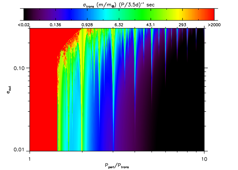
Figure 5: Dispersion, $\sigma_{trans}$, of timing variations of HD 209458b due to perturbations induced by an exterior earth-mass planet with various eccentricities and periods. The color bar has $\sigma_{trans}$ for a planet of mass $m_{\oplus}$ and for a transiting period of 3.5 days. Near the period ratio of 4:3 the system becomes chaotic. The increase in the number of resonance peaks, particularly those beyond the 2:1 resonance, are from higher order terms in the expansion of the Hamiltonian which were truncated for the near-circular case.

When both planets have non-zero eccentricity, the parameter space becomes quite large: the 4 phase space coordinates for each planet, assuming both are edge-on and 2 mass-ratios give 10 free parameters. On resonance, the analysis remains similar to the circular case. The libration amplitude will still be of order $\sim Pj^{-1}$ for the lighter planet and $\sim Pj^{-1}(\mu_{light}/\mu_{heavy})$ for the heavier planet. However, the period of libration will decrease significantly as the eccentricity increases since $P_{lib}\simeq e^{-1/2}\mu^{-1/2}$.

On the secular time-scale, the precession of the orbits will lead to a significant variation in the transit timing (Miralda-Escudé, 2002). The period of precession, $P_{\nu}$, may be driven by other planets, by general relativistic effects, or by a non-spherical stellar potential, but leads to a magnitude of transit timing deviation which just depends on the eccentricity for $P_{\nu}\gg P$. Miralda-Escudé (2002) showed that the maximum deviation for $e\ll 1$ is given by

$$\delta t=\frac{eP}{\pi}$$ (43)

and the timing variations vary with a period that is equal to the period of precession. For arbitrary eccentricity, the maximum deviation is

$$\delta t={P\over 2\pi}\left[\sin^{-1}{y}+\sin^{-1}{z}+\sqrt{2x-x^{2}-x^{4}}\right],$$ (44)

where $x=(1-e^{2})^{1/4}$, $y=(1-x)/e$, and $z=(1-x^{3})/e$ (this is derived from the Keplerian solution with a slowly varying $\varpi$). This approaches $P/2$ as $e\rightarrow 1$. Typically the eccentricity will vary on the secular time-scale, so these expressions only hold as long as the variation in $e$ is much smaller than its mean value.

Rather than systematically studying the entire parameter space, we now investigate several specific cases of known extrasolar planets to demonstrate that detection of this effect should be possible once a transiting multi-planet system is found. Most of these systems have non-zero eccentricities and several are in resonance, causing a significant signal. We summarize the amplitude of the signals of most known multi-planet systems, if they were seen edge-on, in Table 1 (in some cases other planets are present which would cause additional perturbations).

Table 1: Timing variations for known multi-planet systems

System	$P_{in}$ (d)	$P_{out}/P_{in}$	$\sigma_{1}$	$\sigma_{2}$
55 Cnc e, b	2.81	5.21	10.5 s	2.68 s
55 Cnc b, c	14.7	3.02	1.61 h	14.7 h
Ups And b, c	4.62	52.3	1.30 s	1.61 min
Gliese 876	30.1	2.027	1.87 d	14.6 h
HD 74156	51.6	39.2	4.98 min	42.4 min
HD 168443	58.1	29.9	12.9 min	2.62 h
HD 37124	152	9.81	3.43 d	11.2 d
HD 82943	222	2.00	34.9 d	30.7 d
PSR 1257+12 b, c	66.5	1.48	15.2 min	22.3 min
Earth/Jupiter	365	11.9	1.42 min	24.1 s

The extrasolar planetary system Gliese 876 contains two Jupiter-mass planets on modestly eccentric orbits which are near the 2:1 mean-motion resonance, $P_{1}=30.1$d and $P_{2}=61.0$d (Marcy et al., 2001). Due to the small size of the M4 host star, the inner planet has a 1.5 per cent probability of transiting for an observer at arbitrary inclination. The orbital motion involves both mean-motion resonance as well as a secular resonance in which the planets librate about their apsidal alignment. The apsidal alignment is in turn precessing at a rate of $-41^{\circ}$ per year (Laughlin et al., 2004; Nauenberg, 2002; Rivera & Lissauer, 2001; Laughlin & Chambers, 2001). Figure 6 shows the predicted timing variations if this system were seen edge-on and if the planets are coplanar using the orbital elements from Laughlin et al. (2004).

The two most prominent periodicities in Figure 6 are those associated with the 2:1 libration, with a period of roughly 600 days (20 orbits of the inner planet, Laughlin & Chambers, 2001), and the long term precession of the apsidal angle with a period of about 3200 days (110 orbits of the inner planet, corresponding to $-41^{\circ}$ yr^-1). Evaluating equation (43) gives a peak amplitude of 1.4 days for the inner planet and 18 hours for the outer planet which both compare well with the numerical results given that the eccentricities are not constant.

Figure 6: (a) Transit timing variations for Gliese 876 B and (b) Gliese 876 C. The vertical axis is in units of hours, while the horizontal axis is in units of the period of the transiting planet (given in parentheses for reference).

The extrasolar planetary system 55 Cancri contains a set of planets, $b$ and $c$, near the $3$:$1$ resonance having 15 and 45 day periods. There is some evidence for another planet, $d$, in an extremely long orbit, and recently a fourth low mass planet, $e$, was found with a 2.8 day period (McArthur et al., 2004). The planets $e$, $b$, and $c$ have transit probabilities of 12, 4, and 2 per cent, respectively, for an observer at arbitrary inclination. The orbit of planet $b$ is approximately circular while planet $c$ is somewhat eccentric (Marcy et al., 2002). Table 1 gives the amplitude of the variations for the planets. We have ignored planet $e$; however, it is at a large enough semi-major axis to produce a $\sim$ 22 second variation due to light-travel time as the barycenter of the inner binary orbits the barycenter of the triple system were the inner planets transiting.

The double planet system Upsilon Andromedae has a semi-major axis ratio of 14 which is not in a mean-motion resonance (Butler et al., 1999; Marcy et al., 2001). The inner planet has a short period of 4.6 days, and thus a significant probability of transiting of about 12 per cent, but has variations which are too small to currently be detected from the ground or space. The outer planet has much larger transit timing variations due to its smaller velocity, but a much smaller probability of transiting.

The planetary system HD 37124 has two planets with a period ratio of $\sim 10$ and a period of the inner planet of 241 days (Vogt et al., 2000). The outer planet is highly eccentric, $e_{2}=0.69$, and so its periapse passage produces a large and rapid change in the transit timing of the inner planet. If this system were transiting, the variations would be large enough to be detected from the ground. HD 82943 is in a 2:1 resonance giving variations of order the periods of the planets. The pulsar planets are near a 3:2 resonance, which would cause large transit timing variations were they seen to transit the pulsar progenitor star. Finally, alien civilizations observing transits of the Sun by Jupiter would have to have $\sim$ 10 second accuracy to detect the effect of the Earth.

8 Applications

8.1 Detection of terrestrial planets

The possibility of detecting terrestrial planets using the transit timing technique clearly depends strongly on (1) the period of the transiting planet; (2) the nearness to resonance of the two planets; (3) the eccentricities of the planets. The detectability of such planets also depends on the measurement error, the intrinsic noise due to stellar variability, and the number of transit timing measurements. One requirement for the case of an external perturbing planet is that observations should be made over a time longer than the period of the timing variations, which can be longer than the period of the perturbing planet. Ignoring these complications, a rough estimate of detectability can be obtained from comparing the standard deviation of the transit timing with the measurement error.

It is worthwhile to provide a numerical example for the case of a hot Jupiter with a 3 day period that is perturbed by a lighter, exterior planet on a circular orbit in exact 2:1 resonance. The timing deviation amplitude is of order the period (3 days) times the mass ratio (300) or about 3 minutes (equation 41):

$$\delta t=3\left({m_{pert}\over m_{\oplus}}\right){\rm min}.$$ (45)

These variations accumulate over a time-scale of order the period (3 days) times the planet to star mass ratio to the power of $2/3$, which for a transiting planet of order a Jupiter mass is about 5 months (equation 42):

$$t_{cycle}=150\left(m_{trans}\over m_{J}\right)^{-2/3}{\rm days}.$$ (46)

Such a large signal should easily be detectable from the ground. With relative photometric precision of $10^{-5}$ from space or from future ground-based experiments, less massive objects or objects further away from resonance could be detected. The observations could be scheduled in advance and require a modest amount of observing time with the possible payoff of being able to detect a terrestrial-sized planet.

8.2 Comparison to other terrestrial planet search techniques

To attempt a comparison with other transit timing techniques, we have estimated the mass of a planet which may be detected at an amplitude of 10 times the noise for a given technique. We compare three techniques for measuring the mass of planets: (1) radial velocity variations of the star; (2) astrometric measurements; (3) transit timing variations (TTV). We assume that radial velocity measurements have a limit of 0.5 m/s, which is about the highest accuracy that has been achieved from the ground, and may be at the limit imposed by stellar variability (Butler et al., 2004). We assume that astrometric measurements have an accuracy of 1 $\mu$arcsecond which is the accuracy which is projected to be achieved by the Space Interferometry Mission (Ford & Tremaine, 2003; Sozzetti et al., 2003). Finally, we assume that the transit timing can be measured to an accuracy of 10 seconds, which is the highest accuracy of transit timing measurements of HD 209458 (Brown et al., 2001).

We concentrate on HD 209458 since it is the best studied transiting planet. This system is at a distance of 46 pc and has a period of 3.5 days. Figure 7 shows a comparison of the 10-$\sigma$ sensitivity of these three techniques. The solid curve is computed for $m_{trans}=6.7\times 10^{-4}{\rm M_{\odot}}$ and $m_{pert}=10^{-7}{\rm M_{\odot}}$ and both planets on circular orbits. When not trapped in resonance, the amplitude of the timing variations scales as $m_{pert}/m_{0}$, so we scale the results to the mass of the perturber to compute where the timing variations are 100 seconds – this determines the sensitivity. For exact resonance we plot equation (41). The TTV technique is more sensitive than the astrometric technique at semi-major axis ratios smaller than about 2. Off resonance, radial velocity measurements are the technique of choice for this system, while on resonance the TTV is sensitive to much smaller planet masses. Note that in Figure 7 the TTV and astrometric techniques have the same slope at small $P_{pert}/P_{trans}$. This is because the transit timing technique is measuring the reflex motion of the host star due to the inner planet, which is also being measured by astrometry. The solid curve is an upper limit to the minimum mass detectable in HD 209458 since a non-zero eccentricity will lead to larger timing variations (Figure 5) and thus a smaller detectable mass.

Figure 7: Mass sensitivity of various planet detection techniques to secondary planets in HD 209458. The vertical axis is the perturbing planet’s mass in units of ${\rm M_{\odot}}$. The horizontal axis is the period ratio of the planets. The solid line is for the transit timing technique, the dashed line is astrometric, and the dotted line is the radial velocity technique. The large dots are equation (41).

8.3 Breaking the mass-radius degeneracy

In the case that two planets are discovered to transit their host star, measurement of the transit timing variations can break the degeneracy between mass and radius needed to derive the physical parameters of the planetary system. This has been discussed by Seager & Mallén-Ornelas (2003) who use a theoretical stellar mass-radius relation to break this degeneracy. We provide a simplified treatment here to illustrate the nature of the degeneracy and how it can be broken with observations of transit timing variations.

Consider a planetary system with two transiting planets on circular orbits which are coplanar, exactly edge-on, and have measured radial velocity amplitudes. We’ll assume that the star is uniform in surface brightness and that $m_{1},m_{2}\ll m_{0}$. We’ll also assume that the unperturbed periods $P_{1},P_{2}$ can be measured from the duration between transits. Then there are eight physical parameters of interest which describe the system: $m_{0},m_{1},m_{2},R_{0},R_{1},R_{2},a_{1},$ and $a_{2}$ where $R_{i}$ are the radii of the star and planets. Without measuring the transit timing variations, there are a total of ten parameters which can be measured: $K_{1},K_{2},t_{T1},t_{T2},t_{g1},t_{g2},\Delta F_{1},\Delta F_{2},P_{1},$ and $P_{2}$, where $t_{Tj}$ labels the duration of transit from mid-ingress to mid-egress, $t_{gj}$ labels the duration of ingress or egress for planet $j$, $K_{j}$ are the velocity amplitudes of the two planets, and $\Delta F_{j}$ are the relative depths of the transits in units of the uneclipsed brightness of the star (for planet $j$). Although there are more constraining parameters than model parameters, there is a degeneracy since some of the observables are redundant. All of the system parameters can be expressed in terms of observables and the ratio of the mass to radius of the star, $m_{0}/R_{0}$,

$${R_{j}\over R_{0}} = \Delta F_{j}^{1/2}$$ (47)

$${m_{j}\over m_{0}} = K_{j}\left({P_{j}\over\pi t_{Tj}G}\right)^{1/2}\left({m_{0}\over R_{0}}\right)^{-1/2}$$ (48)

$$a_{j} = {P_{j}\over 2\pi}\left({G\pi t_{Tj}\over P_{j}}\right)^{1/2}\left({m_{0}\over R_{0}}\right)^{1/2}$$ (49)

$${R_{0}\over a_{j}} = {\pi t_{Tj}\over P_{j}}$$ (50)

$${R_{j}\over a_{j}} = {\pi t_{gj}\over P_{j}},$$ (51)

where $j=1,2$ labels each planet. From this information alone one can constrain the density of the star (Seager & Mallén-Ornelas, 2003). For the simplified case discussed here,

$$\rho_{*}={3P\over\pi^{2}Gt_{T}^{2}}$$ (52)

for either planet (this differs sligthly from the expression in Seager & Mallén-Ornelas, 2003, since we define the transit duration from mid in/egress). If, in addition, one can measure the amplitude of the transit timing variations of the outer planet, $\sigma_{2}$, then this determines the mass ratio. For the case that the star’s motion dominates the transit timing,

$${m_{1}\over m_{0}}={2\sqrt{2}\pi\sigma_{2}\over P_{2}^{1/3}P_{1}^{2/3}}.$$ (53)

For other cases, the transit timing amplitude can be computed numerically. Then, from the above expression for $m_{i}/m_{0}$ one can find the ratio of the mass to the radius of the star

$${m_{0}\over R_{0}}={1\over 8\pi^{3}G}{P_{1}^{7/3}P_{2}^{2/3}K_{1}^{2}\over t_{T1}\sigma_{2}^{2}}.$$ (54)

Combined with the measurement of the density, this gives the absolute mass and radius of the star. This procedure requires no assumptions about the mass-radius relation for the host star, and in principle could be used to measure this relation. If one can also measure transit timing variations for the inner planet, then an extra constraint can be obtained

$$\sigma_{1}={P_{1}m_{2}\over m_{0}}f(\alpha),$$ (55)

where $f(\alpha)$ is a function derived from averaging equation 74. (Note that the phase of the orbits is needed for this equation, which can be found from the velocity amplitude curve). This provides an extra constraint on the system, and thus will be a check that this procedure is robust.

Clearly we have made some drastically simplifying assumptions which are not true for any physical transit. The inclination of the orbits must be solved for, which can be done from the ratio of the durations of the ingress and transit and the change in flux, as demonstrated by Seager & Mallén-Ornelas (2003). In addition, limb-darkening must be included, and can be solved for with high signal-to-noise data as demonstrated by Brown et al. (2001). Finally, the orbits are not generally circular, so the parameters $e_{j},\varpi_{j},\Omega_{j},\sigma_{j}$, which can be derived from the velocity amplitude measurements, should be accounted for. The general solution is rather complicated and would best be accomplished numerically, but the degeneracy has a similar nature to the circular case and can in principle be broken by the transit timing variations.

9 Effects we have ignored

We now discuss several physical effects that we have ignored, which ought to be kept in mind by observers measuring transit timing variations.

9.1 Light travel time

Deeg et al. (2000) carried out a search for perturbing planets in the eclipsing binary stellar system, CM Draconis, using the changes in the times of the eclipse due to the light travel time to measure a tentative signal consistent with a Jupiter-mass planet at $\sim 1$ AU (their technique would in principle be sensitive to a planet on an eccentric orbit as well, c.f equation 31). The “Römer Effect” due to the change in light travel time caused by the reflex motion of the inner binary is much smaller in planetary systems than in binary stars since their masses and semi-major axes are small, having an amplitude

$$t_{star}={a\over c}{m_{p}\over m_{*}}\approx 0.5{\rm sec}\left({m_{p}\over M_{J}}\right)\left({a_{2}\over 1{\rm AU}}\right)$$ (56)

where $M_{J}$ is the mass of Jupiter and $a_{2}$ is the semi-major axis of the perturbing planet. This effect is present in the absence of deviations from a Keplerian orbit because the inner binary orbits about about the center of mass.

There can also be changes in the timing of the transit as the distance of the transiting planet from the star varies. In this case, the time of transit is delayed by the light travel time between the different locations where the planet intercepts the beam of light from the star. The amplitude of these variations is smaller than the $\sigma$ we have calculated by a factor of $\sim v_{trans}/c$, where $v_{trans}$ is the velocity of the transiting planet. So, only very precise measurements will require taking into account light travel time effects, which should be borne in mind in future experiments (of course the light-travel time due to the motion of the observer in our solar system must be taken into account with current experiments).

9.2 Inclination

We have assumed that the planets are strictly coplanar and exactly edge-on. The first assumption is based on the fact that the solar system is nearly coplanar and the theoretical prejudice that planets forming out of disks should be nearly coplanar. Small non-coplanar effects will change our results slightly (Miralda-Escudé, 2002), while large inclination effects would require a reworking of the theory. Since some extrasolar planetary systems have been found with rather large eccentricities, it is entirely possible that non-coplanar systems will be found as well, a possibility we leave for future studies.

The assumption that the systems are edge-on is based on the fact that a transit can occur only for systems that are nearly edge-on. For small inclinations our formulae will only change slightly, but may result in interesting effects such as a change in the duration of a transit, or even the disappearance of transits due to the motion of the star about the barycenter of the system. On a much longer time-scale (centuries), the precession of an eccentric orbit might cause the disappearance of transits since the projected shape of the orbit on the sky can change. This possibility was mentioned by Laughlin et al. (2004) for GJ 876.

9.3 Other sources of timing “noise”

Aside from the long term effects that have been ignored there are several sources of timing noise that must be included in the analysis of observations of transiting systems. These sources of noise could come from the planet or the host star. If the planet has a moon or is a binary planet then there is some wobble in its position causing a change in both the timing and duration of a transit (Sartoretti & Schneider, 1999; Brown et al., 2001). A moon or ring system may transit before the planet causing a shallower transit to appear earlier or later than it would without the moon (Brown et al., 2001; Schneider, 2003; Barnes & Fortney, 2004). A large scale asymmetry of the planet’s shape with respect to its center of mass might cause a slightly earlier or later start to the ingress or end of egress.

Stellar variability could also make a significant contribution to the noise. Variations in the brightness of the star might affect the accuracy of the measurement of the start of ingress and the end of egress, which are the times that are critical to timing of a transit. Stellar oscillations can cause variations in the surface of the Sun of $\sim 100$ km in regions of size $10^{3-4}$ km, which corresponds to a one second variation for a planet moving at 100 km/s.

9.4 Coverage Gaps

Radial velocities and prior transit lightcurves predict the epoch of future transits and to schedule photometric monitoring for the system of interest. Observational limitations (e.g. bad weather, equipment failure, scheduling requirements) will lead to transits being missed, which in turn will cause inaccuracies in $\sigma$. Since the signal is periodic, $\delta t(t)$ may be straightforward to extract with a few missed transits; however, if the outer planet is highly eccentric, then most of the change in transit timing may occur for a few transits (e.g. HD37124; a similar selection effect occurs in radial velocity searches as discussed by Cumming, 2004). In principle this effect will average out over long observational intervals; however as in this context “long” may mean several decades or more, it will be important to evaluate the effect of coverage gaps on detections over a time-scale of months-years. We will return to this in detail in future work.

We note in passing that the advent of the new astrometric all-sky surveys such as Gaia (Perryman et al., 2001) will provide photometry for $\sim 10^{7}$ stars $>$ 15 mag, with fewer coverage gaps than ground-based observations; we thus expect the detection method by transits alone (section 8.1) to really come into its own over the next two decades. Assuming $\sim$ 0.4 detections (three transits) per 10⁴ stars (c.f. Brown, 2003), we may expect transit lightcurves of perhaps $\sim 1000$ exoplanetary systems over the mission lifetime, greatly aiding the determination of $\sigma$ for these systems. The NASA Kepler mission will also provide uniform monitoring of about $10^{2-3}$ transiting gas giants (Borucki et al., 2003), and if flown, the Microlensing Planet Finder (formerly GEST) will discover $10^{4-5}$ transiting gas giants with uniform coverage (Bennett & et al., 2003).

10 Conclusions

For an exoplanetary system where one or more planets transit the host star the timing and duration of the transits can be used to derive several physical characteristics of the system. This technique breaks the degeneracy between the mass and radius of the objects in the system. The inclination, absolute mass, and absolute radii of the star and planets can be found; in principle this could be used to measure the mass-radius relation for stars that are not in eclipsing binaries.

In addition, TTV can be used to infer the existence of previously undetected planets. We have found that for variations which occur over several orbital periods the strongest signals occur when the perturbing planet is either in a mean-motion resonance with the transiting planet or if the transiting planet has a long period (which, unfortunately, makes a transit less probable). The resonant case is more interesting since the probability of a planet transiting decreases significantly as the semi-major axis becomes large. Using the TTV scheme it is possible to detect earth-mass planets using current observational technologies for both ground based and space based observatories. Data for several transits of HD 209458 could be gathered and studied over a relatively short time due to its small period. Once the existence of a second planet is established one can predict the times at which it would likely transit the host star. Follow-up observations with HST or high-precision ground-based telescopes at those times would increase the likelihood of detecting a transit of the second planet.

If the second planet is terrestrial in nature, this transit timing method may be the only way currently to determine the mass of such planets in other star systems. Astrometry is another possible technique but it may take a decade of technological development before the necessary sensitivity is achieved. In addition, complementary techniques are necessary to probe different parts of parameter space and to provide extra confidence that the detected planets are real, given the likely low signal-to-noise (Gould et al., 2004). For the near future the TTV technique may be the most promising method of detecting earth-mass planets around main sequence stars besides the Sun.

We exhort observers to (1) discover longer period transiting planets (Seagroves et al., 2003) since the signal increases with transiting planet’s period; (2) increase the signal-to-noise of ground based differential photometry (Howell et al., 2003) for more precise measurement of the transit times; and (3) examine their transit data for the presence of perturbing planets (Brown et al., 2001).

The treatment of this problem has ignored many effects which we plan to take into account in a future paper in which we will simulate realistic lightcurves including noise and to fit the simulated data to derive the parameters of the perturbing planet, exploring degeneracies in the period ratio. We will also derive the probability of detecting such systems taking into account various assumptions about the formation, evolution, and stability of extrasolar planets.

11 Acknowledgements

We acknowledge discussions with Peter Goldreich, Man-Hoi Lee, Jean Schneider.

Appendix A Perturbation theory treatment of nearly circular orbits

In this appendix we consider the case of two planets whose orbits are nearly circular and whose timing variations are dominated by changes in eccentricity (see §5). The timing variations can be computed from a Hamiltonian as described in Malhotra (1993a). We keep terms which are first order in the eccentricity because mutual perturbations between the planets induces an eccentricity of order $m_{2}/m_{0}$. To first order in the eccentricities, the Taylor-expanded Hamiltonian is

$$H_{int}= -{Gm_{1}m_{2}\over 2a_{2}}\left[2P-2\alpha\cos{\psi}-e_{1}c^{+}_{0}\cos{\left(\lambda_{1}-\varpi_{1}\right)}\right.$$ (57)

$$+ e_{2}d^{+}_{0}\cos{\left(\lambda_{2}-\varpi_{2}\right)}$$ (58)

$$- e_{1}\sum_{j=1}^{\infty}\left(c^{-}_{j}+\alpha\delta_{j,1}\right)\cos\left((j+1)\lambda_{1}-j\lambda_{2}-\varpi_{1}\right)$$ (59)

$$- e_{1}\sum_{j=1}^{\infty}\left(c^{+}_{j}-3\alpha\delta_{j,1}\right)\cos\left((j-1)\lambda_{1}-j\lambda_{2}+\varpi_{1}\right)$$ (60)

$$+ e_{2}\sum_{j=1}^{\infty}d^{-}_{j}\cos\left(j\lambda_{1}-(j-1)\lambda_{2}-\varpi_{2}\right)$$ (61)

$$+ \left.e_{2}\sum_{j=1}^{\infty}\left(d^{+}_{j}-4\alpha\delta_{j,1}\right)\cos\left(j\lambda_{1}-(j+1)\lambda_{2}+\varpi_{2}\right)\right],$$ (62)

where $\delta_{i,j}$ is the Kronecker delta, $c^{\pm}_{j}=\partial_{\alpha}b^{(j)}_{1/2}\pm 2jb^{(j)}_{1/2}$, $d^{\pm}_{j}=c^{\pm}_{j}+b^{(j)}_{1/2}(\alpha)$, $\alpha=a_{1}/a_{2}$, $b^{(j)}_{1/2}(\alpha)$ is the Laplace coefficient,

$$b^{(j)}_{1/2}(\alpha)={1\over\pi}\int_{0}^{2\pi}d\theta{\cos{j\theta}\over\sqrt{1-2\alpha\cos{\theta}+\alpha^{2}}},$$ (63)

where $\psi=\lambda_{1}-\lambda_{2}$,

$$P=P(\psi,\alpha)=\left(1-2\alpha\cos{\psi}+\alpha^{2}\right)^{-1/2},$$ (64)

and

$$\partial_{\alpha}b^{(j)}_{1/2}(\alpha)\equiv\alpha{\partial\over\partial\alpha}b^{(j)}_{1/2}(\alpha).$$ (65)

This equation includes no secular terms since these are higher order in the eccentricity. Note that since we have only included the first order terms in the eccentricity, the resonant arguments which appear have ratios $j+1$:$j$ and $j$:$j+1$ for the mean longitudes.

The perturbed semi-major axis is given in Malhotra (1993b), and we compute the perturbed eccentricity and longitude of periastron using $h_{1}=e_{1}\sin{\varpi_{1}}$ and $k_{1}=e_{1}\cos{\varpi_{1}}$. Keeping all the resonance terms that exist to first order in the eccentricities gives the equations of motion for $h_{1},k_{1}$,

$$\dot{h}_{1} = -{1\over 2}n_{1}\alpha{m_{2}\over m_{0}}\left[c^{+}_{0}\cos{\lambda_{1}}\right.$$ (66)

$$+ \left.\sum_{j=1}^{\infty}\left\{\left(c^{+}_{j}-3\alpha\delta_{j,1}\right)\cos{[(j-1)\lambda_{1}-j\lambda_{2}]}\right.\right.$$ (67)

$$+ \left.\left.\left(c^{-}_{j}+\alpha\delta_{j,1}\right)\cos{[(j+1)\lambda_{1}-j\lambda_{2}]}\right\}\right],$$ (68)

$$\dot{k}_{1} = {1\over 2}n_{1}\alpha{m_{2}\over m_{0}}\left[c^{+}_{0}\sin{\lambda_{1}}\right.$$ (69)

$$- \sum_{j=1}^{\infty}\left\{\left(c^{+}_{j}-3\alpha\delta_{j,1}\right)\sin{[(j-1)\lambda_{1}-j\lambda_{2}]}\right.$$ (70)

$$- \left.\left.\left(c^{-}_{j}+\alpha\delta_{j,1}\right)\sin{[(j+1)\lambda_{1}-j\lambda_{2}]}\right\}\right].$$ (71)

To find the change in the transit timing we use the orbital elements to compute the variation in $\dot{\theta}_{1}$. To first order in $e_{1}$

$${\dot{\theta}_{1}\over n_{10}}\approx 1+{\delta n_{1}\over n_{10}}+2k_{1}\cos{\left[n_{10}t+\lambda_{10}\right]}+2h_{1}\sin{\left[n_{10}t+\lambda_{10}\right]}.$$ (73)

Since we begin with zero eccentricity, we ignore perturbations to $\lambda$ in the $\sin$ and $\cos$ terms in this equation. As in equation (28) where $\delta\dot{\theta}_{1}=\dot{\theta}_{1}-n_{10}$, we integrate this equation to find

$$\delta t_{1}= 3{m_{2}\over m_{0}}\alpha{n_{1}\over\left(n_{1}-n_{2}\right)^{2}}\left(Q(\psi)-{2\psi K(k)\over\pi(1+\alpha)}-\alpha\sin{\psi}\right)$$ (74)

$$- n_{1}{m_{2}\over m_{0}}\alpha\left[{c^{+}_{0}\over n_{1}^{2}}\sin{(\lambda_{1}-\lambda_{10})}\right.$$ (75)

$$+ \sum_{j=1}^{\infty}{c_{j}^{+}-3\alpha\delta_{j,1}\over(j-1)n_{1}-jn_{2}}\left({\sin{[j\psi]}\over j(n_{1}-n_{2})}-{\sin{[n_{1}t+j\psi_{0}]}\over n_{1}}\right)$$ (76)

$$- \left.\sum_{j=1}^{\infty}{c_{j}^{-}+\alpha\delta_{j,1}\over(j+1)n_{1}-jn_{2}}\left({\sin{[j\psi]}\over j(n_{1}-n_{2})}-{\sin{[n_{1}t-j\psi_{0}]}\over n_{1}}\right)\right],$$ (77)

where $n_{1}$ and $n_{2}$ are taken at their initial values, $\lambda_{10}=\lambda_{1}(t=0)$, $\lambda_{20}=\lambda_{2}(t=0)$, $k=2\sqrt{\alpha}/(1+\alpha)$, $K(k)$ is the complete elliptic integral, $Q(\psi)$ is defined in the appendix of Malhotra (1993b), and we have dropped any terms which vary linearly with time.

A similar calculation can be carried out for perturbations by a planet interior to the transiting planet,

$$\delta t_{2}= -3\frac{m_{1}}{m_{0}}\frac{n_{2}}{(n_{1}-n_{2})^{2}}\left(Q(\psi)-\frac{2\psi K(k)}{\pi(1+\alpha)}-\alpha\sin(\psi)\right)$$ (78)

$$+ n_{2}\frac{m_{1}}{m_{0}}\left[\frac{d_{0}^{+}}{n_{2}^{2}}\sin[\lambda_{2}-\lambda_{20}]\right.$$ (79)

$$+ \sum_{j=1}^{\infty}\frac{d_{j}^{+}-4\alpha\delta_{j,1}}{(jn_{1}-(j+1)n_{2})}\left(\frac{\sin[j\psi]}{j(n_{1}-n_{2})}-\frac{\sin[n_{2}t+j\psi_{0}]}{n_{2}}\right)$$ (80)

$$- \left.\sum_{j=1}^{\infty}\frac{d_{j}^{-}}{(jn_{1}-(j-1)n_{2})}\left(\frac{\sin[j\psi]}{j(n_{1}-n_{2})}-\frac{\sin[n_{2}t-j\psi_{0}]}{n_{2}}\right)\right]$$ (81)

A comparison of these equations to numerical calculations is shown in Figure 8. The planets are on initially circular orbits with a semi-major axis ratio of 1.8, or period ratio of 2.4. The masses are equal and the planets start aligned along the line of sight at the first transit.

Figure 8: Deviations from uniform times between transits for a transiting outer planet with semi-major axis ratio 1.8. Crosses represent the analytic result, equation (78), while the diamonds are from a numerical integration of the equations of motion. The horizontal axis is the number of the transit, while the vertical axis shows the timing differences in units of $P_{1}$, the period of the inner perturbing planet, multiplied by $m_{0}/m_{pert}$.

In the case that the semi-major axis dominates the timing variations, one can take perturbed value of the eccentricity ($h$ and $k$) and compute the change in semi-major axis due to these eccentricities. The result is a double-series over resonant terms, so we do not reproduce it here.

References

- Alonso et al. (2004) Alonso R., Brown T. M., Torres G., Latham D. W., Sozzetti A., Mandushev G., Belmonte J. A., Charbonneau D., Deeg H. J., Dunham E. W., O’Donovan F. T., Stefanik R. P., 2004, astro-ph/0408421
- Barnes & Fortney (2004) Barnes J. W., Fortney J. J., 2004, astro-ph/0409506
- Bennett & et al. (2003) Bennett D. P., et al. 2003, in Future EUV/UV and Visible Space Astrophysics Missions and Instrumentation. Edited by J. Chris Blades, Oswald H. W. Siegmund. Proceedings of the SPIE, Volume 4854, pp. 141-157 (2003). The Galactic Exoplanet Survey Telescope (GEST). pp 141–157
- Borkovits et al. (2003) Borkovits T., Érdi B., Forgacs-Dajka E., Kovacs T., 2003, A&A, 398, 1091
- Borucki et al. (2003) Borucki W. J., Koch D. G., Lissauer J. J., Basri G. B., Caldwell J. F., Cochran W. D., Dunham E. W., Geary J. C., Latham D. W., Gilliland R. L., Caldwell D. A., Jenkins J. M., Kondo Y., 2003, in Future EUV/UV and Visible Space Astrophysics Missions and Instrumentation. Edited by J. Chris Blades, Oswald H. W. Siegmund. Proceedings of the SPIE, Volume 4854, pp. 129-140 (2003). The Kepler mission: a wide-field-of-view photometer designed to determine the frequency of Earth-size planets around solar-like stars. pp 129–140
- Bouchy et al. (2004) Bouchy F., Pont F., Santos N. C., Melo C., Mayor M., Queloz D., Udry S., 2004, astro-ph/0404264
- Brown et al. (2001) Brown T., Charbonneau D., Gilliland R. L., Noyes R. W., A. B., 2001, ApJ, 552, 699
- Brown (2003) Brown T. M., 2003, ApJL, 593, L125
- Butler et al. (2004) Butler P., Vogt S. S., Marcy G. W., Fischer D. A., Wright J. T., Henry G. W., Laughlin G., Lissauer J., 2004, astro-ph/0408587
- Butler et al. (1999) Butler R. P., Marcy G. W., Fischer D. A., Brown T. M., Contos A. R., Korzennik S. G., Nisenson P., Noyes R. W., 1999, ApJ, 526, 916
- Charbonneau (2003) Charbonneau D., 2003, astro-ph/0312252
- Charbonneau et al. (2000) Charbonneau D., Brown T., Latham D., Mayor M., 2000, ApJ, 529, L45
- Cumming (2004) Cumming A., 2004, astro-ph/0408470
- Deeg et al. (2000) Deeg H. J., Doyle L. R., Kozhevnikov V. P., Blue J. E., Martin E. L., Schneider J., 2000, A&A, 358, L5
- Dobrovolskis & Borucki (1996) Dobrovolskis A. R., Borucki W. J., 1996, American Astronomical Society Division of Planetary Science Meeting, 28, 1208
- Fischer et al. (2001) Fischer D. A., Marcy G. W., Butler R. P., Vogt S. S., Frink S., Apps K., 2001, ApJ, 551, 1107
- Ford & Tremaine (2003) Ford E. B., Tremaine S., 2003, PASP, 115
- Gould et al. (2004) Gould A., Gaudi B. S., Han C., 2004, ArXiv Astrophysics e-prints
- Horne (2003) Horne K., 2003, in ASP Conf. Ser. 294: Scientific Frontiers in Research on Extrasolar Planets Status aand Prospects of Planetary Transit Searches: Hot Jupiters Galore
- Howell et al. (2003) Howell S. B., Everett M. E., Tonry J. L., Pickles A., Dain C., 2003, PASP, 115, 1340
- Konacki et al. (2003) Konacki M., Torres G., Jha S., Sasselov D. D., 2003, Nature, 421, 507
- Konacki et al. (2004) Konacki M., Torres G., Sasselov D. D., Pietrzynski G., Udalski A., Jha S., Ruiz M. T., Gieren W., Minniti D., 2004, astro-ph/0404541
- Laughlin et al. (2004) Laughlin G., Butler R. P., Fischer D. A., Marcy G. W., Vogt S. S., Wolf A. S., 2004, astro-ph/0407441
- Laughlin & Chambers (2001) Laughlin G., Chambers J. E., 2001, ApJ, 551, L109
- Malhotra (1993a) Malhotra R., 1993a, in Planets Around Pulsars, ASP Conference Proceedings, J. A. Phillips, J. E. Thorsett, and S. R. Kulkarni, eds., p. 89
- Malhotra (1993b) Malhotra R., 1993b, ApJ, 407, 266
- Mandel & Agol (2002) Mandel K., Agol E., 2002, ApJ, 529, L45
- Marcy et al. (2001) Marcy G. W., Butler R. P., Fischer D., Vogt S. S., Lissauer J. J., Rivera E. J., 2001, ApJ, 556, 296
- Marcy et al. (2002) Marcy G. W., Butler R. P., Fischer D. A., Laughlin G., Vogt S. S., Henry G. W., Pourbaix D., 2002, ApJ, 581, 1375
- McArthur et al. (2004) McArthur B. E., Endl M., Cochran W. D., Benedict G. F., Fischer D. A., Marcy G. W., Butler R. P., Naef D., Mayor M., Queloz D., Udry S., Harrison T. E., 2004, astro-ph/0408585
- Miralda-Escudé (2002) Miralda-Escudé J., 2002, ApJ, 564, 1019
- Murray & Dermott (1999) Murray C. D., Dermott S. F., 1999, Solar System Dynamics. (Cambridge: Cambridge Univ. Press)
- Nauenberg (2002) Nauenberg M., 2002, ApJ, 568, 369
- Pan & Sari (2004) Pan M., Sari R., 2004, AJ, 128, 1418
- Perryman (2000) Perryman M. A. C., 2000, Rep. Prog. Phys., 63, 1209
- Perryman et al. (2001) Perryman M. A. C., de Boer K. S., Gilmore G., Høg E., Lattanzi M. G., Lindegren L., Luri X., Mignard F., Pace O., de Zeeuw P. T., 2001, A&A, 369, 339
- Pont et al. (2004) Pont F., Bouchy F., Queloz D., Santos N., Melo C., Mayor M., Udry S., 2004, astro-ph/0408499
- Rivera & Lissauer (2001) Rivera E. J., Lissauer J. J., 2001, ApJ, 558, 392
- Santos et al. (2004) Santos N. C., Bouchy F., Mayor M., Pepe F., Queloz D., Udry S., Lovis C., Bazot M., Benz W., Bertaux J. ., Curto G. L., Delfosse X., Mordasini C., Naef D., Sivan J. ., Vauclair S., 2004, astro-ph/0408471
- Sartoretti & Schneider (1999) Sartoretti P., Schneider J., 1999, A&AS, 134, 553
- Schneider (2003) Schneider J., 2003, SF2A-2003: Semaine de l’Astrophysique Frangaise, meeting held in Bordeaux, France, June 16-20, 2003. Eds.: F. Combes, D. Barret and T. Contini. EdP-Sciences, Conference Series, p. 75
- Seager & Mallén-Ornelas (2003) Seager S., Mallén-Ornelas G., 2003, ApJ, 585
- Seagroves et al. (2003) Seagroves S., Harker J., Laughlin G., Lacy J., Castellano T., 2003, PASP, 115, 1355
- Sozzetti et al. (2003) Sozzetti A., Casertano S., Brown R. A., Lattanzi M. G., 2003, PASP, 115
- Vogt et al. (2000) Vogt S. S., Marcy G. W., Butler R. P., Apps K., 2000, ApJ, 536, 902
- Wisdom (1980) Wisdom J., 1980, AJ, 85, 1122