Leninskii prosp., 53, Moscow, 119991, Russia
11email: beskin@lpi.ru 22institutetext: Moscow Institute of Physics and Technology,
Institutskii per., 9, Dolgoprudny, 141700, Russia
22email: chekhovs@lpi.ru
Two-dimensional structure of thin transonic discs: theory and observational manifestations
We study the two-dimensional structure of thin transonic accretion discs in the vicinity of black holes. We use the hydrodynamical version of the Grad-Shafranov equation and focus on the region inside the marginally stable orbit (MSO), . We show that all components of the dynamical force in the disc become significant near the sonic surface and especially important in the supersonic region. Under certain conditions, the disc structure is shown to be far from radial, and we review the affected disc properties, in particular the role of the critical condition at the sonic surface: it determines neither the accretion rate nor the angular momentum in the accretion disc. Finally, we present a simple model explaining quasi-periodical oscillations that have been observed in the infrared and X-ray radiation of the Galactic Centre.
Key Words.:
hydrodynamics – accretion, accretion disks – black hole physics1 Introduction
The investigation of accretion flows near black holes (BHs) is undoubtedly of great astrophysical interest. Substantial energy is released near BHs, and general relativity effects, attributable to strong gravitational fields, show up there. Depending on external conditions, both quasi-spherical and disc accretion flows can be realized.
The studies of thin disc accretion span more than three decades. Many results were included in textbooks (Shapiro & Teukolsky 1983; Lipunov 1992). Lynden-Bell (1969) was the first to point out that supermassive BHs surrounded by accretion discs could exist in galactic nuclei. Subsequently, a theory for such discs was developed that is now called standard model, or the model of the disc (Shakura 1972; Shakura & Sunyaev 1973; Novikov & Thorne 1973).
According to standard model, if the accreting gas temperature is low enough for the speed of sound to be much lower than the Keplerian rotation velocity matter forms a thin equilibrium disc and moves in nearly circular orbits with the Keplerian velocity where is the black hole mass and is the gravitational constant. The disc thickness within this model is determined by the balance of gravitational and accreting matter pressure forces,
| (1) |
Minor friction between rotating gas layers leads to the loss of angular momentum, so that the accreting matter gradually approaches the compact object; this motion only slightly disturbs the vertical balance111Let the vertical, or transversal, direction be a -direction in the spherical system of coordinates with the half-line being aligned with the angular momentum vector of the infalling matter. Then, the longitudinal direction is a radial one. and is commonly considered a small perturbation. To account for this phenomenon, standard model introduces a phenomenological proportionality coefficient between the viscous stress tensor and the pressure , As a result, the radial velocity can be evaluated as
| (2) |
so that for the radial velocity is much lower than both the Keplerian velocity and the speed of sound.
The foregoing is valid far from the compact object where the relativistic effects are unimportant. As for the inner regions of the accretion disc, the general relativity effects lead to at least two new qualitative phenomena. First, there are no stable circular orbits at small radii, for a non-rotating BH; is the radius of the marginally stable orbit (MSO) and is the BH gravitational radius. This means that the accreting matter, that falls into the region rapidly approaches the BH horizon,222In the dynamic time . no matter if the viscosity is present. Second, thin disc accretion on to BHs is always transonic. This results from the fact that, according to (2), the flow is subsonic outside the MSO, , while at the horizon the flow is to be supersonic (Beskin 1997). Therefore, the study of inner accretion disc regions requires consistent analysis of transonic flows.
Transonic accretion on to BHs has been the subject of many research publications. Of crucial importance was the paper by Paczyński & Bisnovatyi-Kogan (1981) who formulated equations of motion in terms of radial derivatives only: they used quantities averaged over the disc thickness. Subsequently, many authors considered only such one-dimensional models. In most cases, the model potential of Paczyński & Wiita (1980), which simulates the properties of the strong gravitational field of a centrally symmetric BH, was used (Abramowicz et al. 1988; Papaloizou & Szuszkiewicz 1994; Chen et al. 1997; Narayan et al. 1997; Artemova et al. 2001). The Schwarzschild and Kerr metrics, that describe the gravitational field of axisymmetric BHs, were far more rare (Riffert & Herold 1995; Peitz & Appl 1997; Beloborodov 1998; Gammie & Popham 1998a, b). As for the two-dimensional structure, it was investigated mostly only numerically and only for thick discs (Papaloizou & Szuszkiewicz 1994; Igumenshchev & Beloborodov 1997; Balbus & Hawley 1998; Krolik & Hawley 2002).
Therefore, for thin accretion discs basic results were obtained in terms of the one-dimensional approach. However, the procedure for averaging over the disc thickness, which is likely to be valid in the region of stable orbits, in fact requires a more serious analysis. In our view, it is the assumption that the transverse velocity may always be neglected in thin accretion discs, i.e. that the disc thickness is always determined by (1), that is the most debatable. This assumption is widely used, explicitly or implicitly, virtually in all papers devoted to thin accretion discs (see the papers cited above and Abramowicz & Zurek 1981; Chakrabarti 1996).
Abramowicz et al. (1997) pointed out the importance of allowing for the transverse velocity in the inner accretion disc regions. They argued that the transverse component of the dynamical force has the same asymptotic near the equatorial plane as the transversal components of the gravitational and pressure forces (under the natural assumption in the limit ). Therefore, the fact that the transversal velocity vanishes on the equator by no means implies that may be ignored. However, in the end the authors concluded that for thin discs the dynamical term may still be disregarded so that the accretion disc thickness can be determined from the balance of the gravitational force and the pressure gradient up to the BH horizon. We show that this conclusion is inapplicable for the class of problems we consider below.
To refine the issue, it may be fruitful to recall the simplest case of transonic accretion, namely ideal spherically symmetric accretion (Bondi 1952). Far outside the sonic surface in such a flow the dynamical term is negligible in comparison with the pressure gradient and the gravitational force. However, all the terms become of the same order of magnitude near the sonic surface. Moreover, after passing the sonic surface, the motion of matter differs little from free-fall, therefore the pressure gradient no longer affects the dynamics of accreting matter. This makes it seem unreasonable to determine the disc thickness from (1), at least in the supersonic region.
However, equation (1) can be easily modified to account for dynamical forces. Indeed, we have at the border of the disc
| (3) |
where . Now assuming linear dependence of on for we obtain
| (4) |
With this in hand the dynamical term can be written as
| (5) |
Now, assuming and using (5), the -component of the Euler equation, divided by can be written as
| (6) |
where the two terms in the l.h.s. correspond to the dynamical force components and respectively. The r.h.s. of (6) corresponds to the discrepancy between the centrifugal force and the pressure force whose absolute value is evaluated as This discrepancy was postulated to vanish in (1).
Accounting for the dynamical forces, equation (6) is a simple qualitative analogue of second-order Grad-Shafranov equation (14) and allows significant disc thickness deviations from the value given by conventional prescription (1). For instance, nondimensionalizing equation (6) yields the characteristic radial scale of change of near the sonic surface , Consistently, by (3) it follows that which indeed indicates a rapid change of the disc thickness. Naturally, in the region of stable orbits in a similar way we get and which justifies the usage of conventional prescription (1) outside the MSO.
The existence of the small longitudinal scale is one of the key results of this paper. Note also that since (6) is a second-order differential equation for there in fact exist two additional degrees of freedom, frequently overlooked before, and only one of the two is fixed by the critical condition at the sonic surface. This hints that the critical condition determines neither the accretion rate nor the angular momentum in the disc but only imposes a restriction on the function i.e. on the form of the flow, near the sonic surface.
In this paper we purposefully consider extreme boundary conditions with radial inflow velocity at the MSO being far smaller than the speed of sound. This allows us to perform the study of the problem analytically. Moreover, the results turn out to be almost independent of the radial inflow velocity, and in the end the observational predictions of our model depend only on the the black hole mass and its angular momentum and are totally independent of the inflow velocity and the speed of sound.
Although our model might not be realized in Nature as is, it – as any other analytical model – bolsters our fundamental understanding of the physical process. Namely, this model offers an insight into the fundamental properties we might lose if we do not allow for the transversal velocity in thin accretion discs. This is the first step to understanding the physics of the critical condition at the sonic surface and its influence on the global disc structure.
In the next section we introduce the reader to the hydrodynamical version of the Grad-Shafranov equation in the Schwarzschild metric as well as derive some useful relations. In sections 3 and 4 we sequentially study the subsonic and the sonic surface regions. Section 5 presents the study of the supersonic flow for the case of a spinning BH, i.e. Kerr metric, followed by the discussion of its applications to the explanation of quasi-periodical oscillations detected in the infrared and X-ray observations of the Galactic Centre (section 6).
2 Basic equations
We consider thin disc accretion on to a BH in the region where there are no stable circular orbits. As argued above, the contribution of viscosity should no longer be significant here. Hence we may assume that ideal hydrodynamics approach is suitable well enough for describing the flow structure in this inner area of the accretion disc. Below, unless specifically stated, we consider the case of a non-spinning BH, i.e. use the Schwarzschild metric, and use a system of units with We measure radial distances in the units of , the BH mass.
In Boyer-Lindquist coordinates the Schwarzschild metric is (Landau & Lifshits 1987a)
| (7) |
where
| (8) |
Here and below indices without caps denote vector components with respect to the coordinate basis in ‘absolute’ three-dimensional space, and indices with caps denote their physical components. The symbol always represents covariant derivative in ‘absolute’ three-dimensional space with metrics (8).
We reduce our discussion to the case of axisymmetric stationary flows. This makes it possible to introduce a stream function which defines the physical poloidal -velocity component as
| (9) |
where is the particle concentration in the comoving reference frame. The surfaces const determine the streamlines of the matter ( corresponds to the streamline ).
For an ideal flow there are three integrals of motion conserved along the streamlines, namely entropy,
| (10) | |||
| energy flux, | |||
| (11) | |||
| and the -component of angular momentum, | |||
| (12) | |||
where is relativistic enthalpy; is internal energy density, is pressure.
As a result the relativistic Euler equation (Frolov & Novikov 1998)
| (13) |
in which indices and take on and values, can be rewritten in the form of the Grad-Shafranov scalar equation for (Beskin 1997),
| (14) |
where the derivative acts on all the variables except the quantity . The equation above contains three integrals , , and Here
| (15) | ||||
| (16) | ||||
| and the thermodynamical function is defined as | ||||
| (17) | ||||
Equation (14) contains the only singular surface – the sonic surface which is defined by the condition . At this surface the equation changes its type from elliptical to hyperbolical.
To close the system, we need to supply the Grad-Shafranov equation with the relativistic Bernoulli equation, , which now becomes
| (18) | ||||
| After using definition (9) we reach | ||||
| (19) | ||||
For the sake of simplification we adopt the polytropic equation of state so that temperature and sound velocity can be written as (Shapiro & Teukolsky 1983)
| (20) |
Since the disc is thin, (see (1)). Therefore we can write where is non-relativistic enthalpy and is particle mass. For an ideal gas with the function can be shown to have a quite definite form
| (21) |
which for the case of the polytropic equation of state can be obtained from (20) and the thermodynamical relationship .
3 Subsonic flow
In this section we show that the role of the dynamical terms becomes dominant with approach to the sonic surface . The problem of passing through the sonic surface and the supersonic flow structure are dealt with later in this paper. Here we limit our discussion to the subsonic region only, where the poloidal velocity is far lower than the sound velocity (as we assume in Sec. 1, the condition holds at the MSO, and in this section we always neglect the terms of the order of or higher). We can simplify Grad-Shafranov hydrodynamic equation (14) in this limit by neglecting terms proportional to :
| (22) |
The resulting equation describes the subsonic flow and is elliptical. Hence, it contains no critical surfaces, and our problem requires five boundary conditions: three conditions determine the integrals of motion and the two remaining ones are the boundary conditions for the second-order Grad-Shafranov equation.
Following Sec. 1, we assume that the -disc theory holds outside the MSO. We adopt the flow velocity components, which this theory yields on the MSO 333A nearly parallel inflow with small radial velocity (2). as the first three boundary conditions for our problem. For the sake of simplicity we consider the radial velocity, which is responsible for the inflow, to be constant at the surface and equal to and the toroidal velocity to be exactly equal to that of a free particle revolving at :444 For a free particle revolving at around a non-spinning BH we have , , (Landau & Lifshits 1987a).
| (23) | ||||
| (24) | ||||
| (25) |
where accounts for the fact that the flow is parallel555Note that the parallel flow is not exactly the same as the radial one. at the MSO. The angular variable is counted off from the equator in the vertical direction.
For the sake of convenience, we also introduce another angular variable , a Lagrange coordinate of streamlines. This is a function of streamlines. For each streamline, it gives the streamline’s -coordinate at the MSO In other words, both points and belong to the same streamline. Further, noting that and using (9) and (23), we arrive at
| (26) |
Next, we assume that the sound velocity is constant at the surface this yields the fourth boundary condition
| (27) |
In the case of polytropic equation of state this means that both the temperature and the relativistic enthalpy are also constant at the surface , i.e.:
| (28) | ||||
| (29) |
Therefore boundary conditions (23) – (25) and (27) directly determine the invariants and ,
| (30) | ||||
| (31) |
where and (see footnote 4).
Condition (30) allows us to rewrite the Grad-Shafranov equation in an even simpler form,
| (32) |
At the r.h.s. of equation (32) can be shown to describe the transversal balance of the pressure force and the effective potential, whereas the l.h.s. corresponds to the dynamical term which is times larger than each of the terms in the r.h.s. and thus may be dropped (Beskin et al. 2002). It is natural therefore to choose entropy from the condition of the transversal balance of forces at the surface
| (33) |
where the value of is determined by (31). This yields the last, fifth, boundary condition
| (34) |
whence owing to (21) we have at the standard shape of concentration,
| (35) |
(to be exact, ). Now with the help of (26), invariants (30), (31), and (34) can be expressed in terms of , therefore the Grad-Shafranov equation does contain the only unknown function .
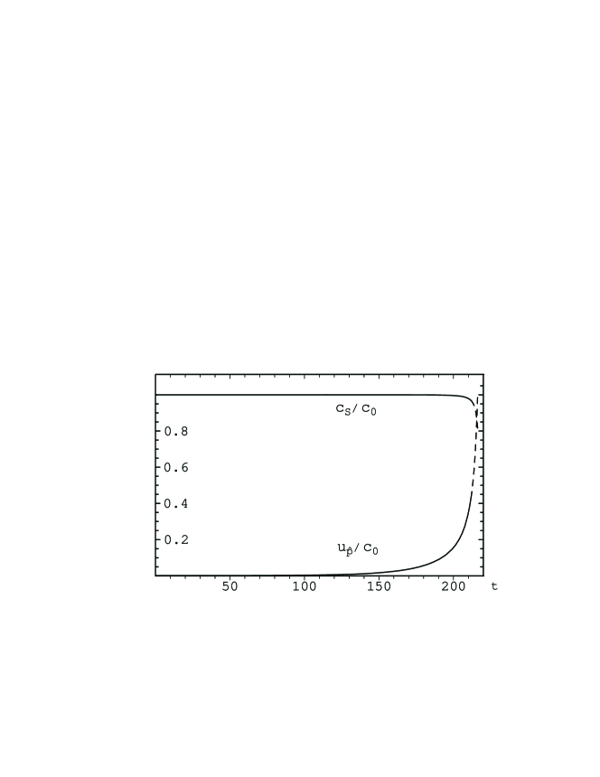
The disc streamlines profile obtained from numerical computation of equation (32) is shown in Fig. 1; the profiles of radial velocity and sound speed are shown in Fig. 2. In the subsonic region, , the disc thickness rapidly diminishes, and at the sonic surface we have so that we cannot neglect the dynamical force there (Beskin et al. 2002).
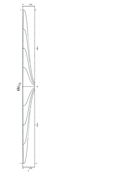
This can be readily derived from qualitative consideration as well. For , i.e. for non-relativistic temperature, we obtain from (18) and (20),
| (36) |
The quantity
| (37) |
is the poloidal four-velocity of a free particle having zero poloidal velocity at the MSO. Assuming and neglecting in (37), we find the velocity of sound in the sonic point , :
| (38) |
Since entropy remains constant along the streamlines, the gas concentration at the sonic surface slightly differs666Note that the concentration, certainly, changes from one streamline to another. from the gas concentration at the MSO. In other words, the subsonic flow can be considered incompressible to a zeroth approximation.777The same is true for spherically symmetric Bondi accretion (Shapiro & Teukolsky 1983). It is important that this conclusion holds not only in the equatorial plane because the additional term in (36) is also of the order of for the range of angles corresponding to the representative disc thickness, (see (35)). Since the density remains almost constant and the poloidal velocity increases from to , i.e. changes over several orders of magnitude for the disc thickness should change in the same proportion due to the continuity equation:
| (39) |
Thus, purely radial motion approximation is inapplicable in the vicinity of the sonic surface, and both components of the dynamical force become comparable to the pressure gradient near the sonic surface (Beskin et al. 2002),
| (40) |
with the position of the sonic surface being determined by
| (41) |
where the logarithmic factor
| (42) |
and the radial logarithmic derivative of concentration near the sonic surface being estimated as
| (43) |
In other words, if there appears a nonzero vertical velocity component, the dynamical term cannot be neglected in the vertical force balance near the sonic surface. This property is apparently valid for arbitrary radial velocities of the flow, i.e. even if the transverse contraction of the disc is not so pronounced.
4 Transonic flow
In order to verify our conclusions we consider the flow structure in the vicinity of the sonic surface in more detail. Since the smooth transonic flow is analytical at a singular point (Landau & Lifshits 1987b), we can write
| (44) | ||||
| (45) |
where . Here we assume that all the three invariants and are given by boundary conditions (30), (31), and (34) respectively. Hence, the problem needs only one more boundary condition.
Full stream equation (14) may be written as
| (46) |
Neglecting spatial derivatives of here (this can be done in the vicinity of the sonic surface for as is shown later) we get an equation with a form similar to (32), but this time the equation can be used in the vicinity of the sonic surface. Now comparing the appropriate coefficients in Bernoulli (18) and full stream equation (46) we obtain neglecting terms of the order of (see the Appendix for the exact values),
| (47) | ||||
| (48) | ||||
| (49) | ||||
| (50) | ||||
| (51) |
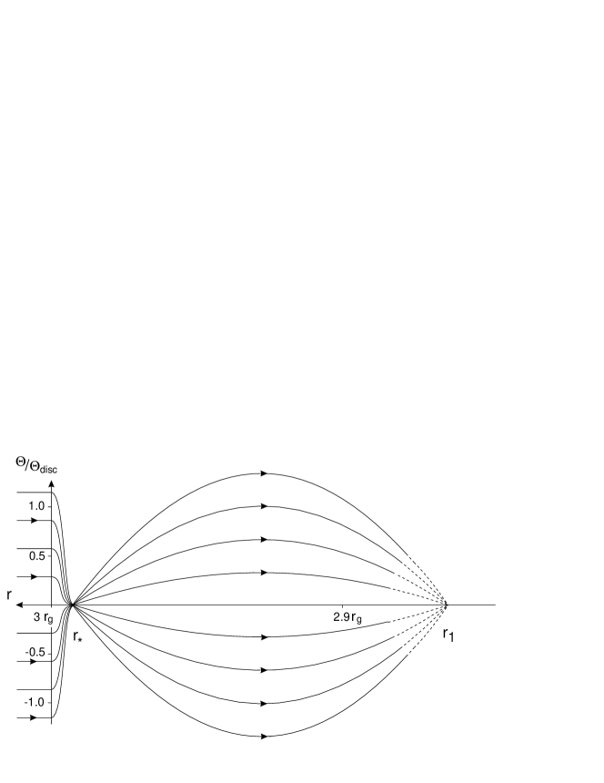
where . As we see, coefficients (47) – (51) are expressed through radial logarithmic derivative (which we specify according to (43) as the fourth boundary condition). They have clear physical meaning. So, gives the compression of streamlines: . In agreement with (39) we have . Further, corresponds to the slope of the streamlines with respect to the equatorial plane. As , the compression of streamlines finishes somewhere before the sonic surface, so inside the sonic radius the streamlines diverge. On the other hand, because , for the divergency is still very weak. Hence in the vicinity of the sonic surface the flow has the form of the standard nozzle (see Fig. 3).

Finally, since , the transverse scale of the transonic region is the same as the longitudinal one. This means that the transonic region is essentially two-dimensional (a well-known fact for a nozzle, see e.g. Landau & Lifshits (1987b)), and it is impossible to analyze it within the standard one-dimensional approximation.
Since the transonic flow in the form of a nozzle has longitudinal and transversal scales of one order of magnitude, near the sonic surface we have i.e.
| (52) |
Hence, for thin discs this longitudinal scale is always much smaller than the distance from the BH, . Only by taking the transversal velocity into account do we retain the small longitudinal scale This scale is left out during the standard one-dimensional approach.
We stress that taking the dynamical force into account is indeed extremely important. This is because, unlike zero-order standard disc thickness prescription (1), the Grad-Shafranov equation has second order derivatives, i.e. contains two additional degrees of freedom. This means that the critical condition only fixes one of these degrees of freedom (e.g. imposes some limitations on the form of the flow) rather than determines the angular momentum of the accreting matter.
Connecting the sonic characteristics with the physical boundary conditions on the MSO is rather difficult (for this we have to know all the expansion coefficients in (44) and (45)). In particular, we cannot formulate the restriction on five boundary conditions (23) – (25), (27), and (34) resulting from the critical condition on the sonic surface. Nevertheless, estimate (43) of makes sure that we know the parameter to a high enough accuracy. Then, according to (47) – (51), all other coefficients can be determined exactly.
5 Supersonic flow
Since the pressure gradient becomes insignificant in the supersonic region, the matter moves here along the trajectories of free particles. Neglecting the term in the -component of relativistic Euler equation (Frolov & Novikov 1998), we have (compare to Abramowicz et al. 1997)
| (55) |
Here, using the conservation law of angular momentum, can be easily expressed in terms of radius: . We also introduce dimensionless functions and :
| (56) | ||||
| (57) |
Using (55) and the definitions above, we obtain an ordinary differential equation for which could be solved if we knew :
| (58) |
From (18) we have as . On the other hand, for . Therefore, the following approximation should be valid throughout the region,
| (59) |
Equation (58) governs the supersonic flow structure for the case of a non-spinning BH. To get a better match with observations (cf. Sec. 6), we also consider a more general case of a spinning BH, i.e. a Kerr BH with non-zero specific angular momentum . After some calculations, equation (58) can be generalized to the Kerr metric with a strikingly simple form,
| (60) |
Here and are the specific energy and the angular momentum of a free particle rotating at the MSO respectively (see e.g. Shapiro & Teukolsky 1983), and is a straightforward generalization of to the Kerr case. For the Schwarzschild BH (, , ) equation (60) reduces back to (58).
Integrating (60), we obtain
| (61) |
where . In the equation above, has been to a good accuracy substituted for the integration constant : for just below the function is positive reflecting the fact that the flow diverges; then, corresponds to the point where the divergency finishes, and the flow starts to converge.
The results of numerical calculations are presented in Fig. 4. In the supersonic region the flow performs transversal oscillations about the equatorial plane, their frequency independent of their amplitude. We see as well that the maximum thickness of the disc in the supersonic (and, hence, ballistic) region, which is controlled by the transverse component of the gravitational force, actually coincides with the disc thickness within the stable orbits region, , where standard estimate (1) is correct.
Once diverged, the flow converges once again at a ‘nodal’ point closer to the BH. The radial positions of the nodes are given by the implicit formula i.e.
| (62) |
where is the node number; the node with corresponds to the sonic surface. In this formula the sonic radius can be to a good accuracy approximated by for (see (41)). The expression for can be found in most textbooks (Shapiro & Teukolsky 1983).
Note that equations (58) and (60) are inapplicable in the very vicinity of the nodes where the pressure gradient cannot be neglected. There may also be an additional energy release because the shock fronts (and, hence, extra sonic surfaces) are inevitably to appear there. These factors can reduce the amplitude of the disc thickness oscillations. Accurate analysis of these factors lies beyond the scope of this paper, and we do not prolong the streamlines to the region in Fig. 4. Nevertheless, it is quite natural to suppose that the nodes positions are not significantly affected by the dissipative processes, and our simple approach may give us a good qualitative understanding of the supersonic flow structure as long as we are interested in general properties of the flow.
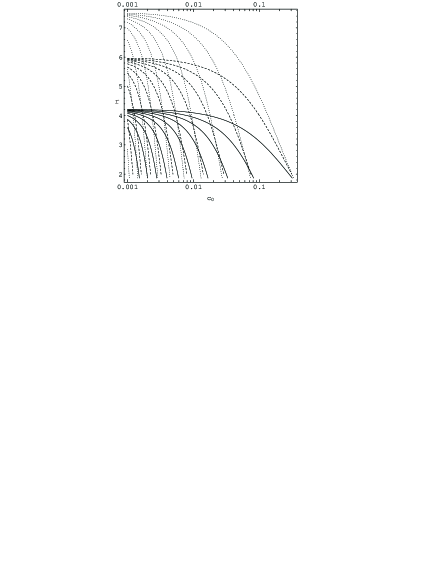
Figure 5 shows the positions of nodes for different values of (the positions do not depend on for ) and the BH spin parameter .
Travel time between the nodes, which is in some sense similar to the half-period of vertical epicyclic oscillations, proves to have weak dependence on both and . This fact provides a means for testing the theory via observations, and we do this in the following section.
6 Applications to observations
6.1 General ideas
Our initial interest in researching into our model’s application to observations was kindled by the publication by Genzel et al. (2003) of the infrared observations of the Galactic Centre (GC): one of the flares obviously showed a number of peaks at time intervals chirping with time (see their Fig. 2e), and this is exactly what we would expect within our model. In this section we measure physical radial distances in the units of and time intervals in the units of .
Suppose some perturbation in the disc (a ‘chunk’) approaches the MSO. We expect to observe radiation coming from the chunk with the period of its orbital motion,
| (63) |
where is the angular momentum per unit mass of the BH and is the estimate of the distance from the BH to the chunk. After a number of rotations, the chunk reaches the MSO and passes through the nodal structure derived earlier (cf. Sec. 5) generating a flare. Each time the chunk passes through a node, it probably generates some additional radiation, and therefore the flare is likely to consist of several peaks. We believe that it is these peaks that were discovered in the infrared and X-ray observations of the GC (Genzel et al. 2003; Aschenbach et al. 2004).
We stress that this section is quite independent of other parts of this work. Qualitatively, our model’s only assumptions are the small thickness of the disc and the divergency of the flow in the supersonic region (the increase of disc thickness with decreasing radius). The latter is guaranteed provided that the flow has the nozzle-like structure (see Sec. 4) near the sonic point.
6.2 Finding the periods
The time interval between the detection of two subsequent peaks (-th and -th) equals the time it takes for the chunk to pass between the two corresponding adjacent nodes (-th and -th), , plus the difference in travel times to the observer for the radiation coming from these two nodes, :
| (64) |
can also be thought of as the index of observed time intervals (counting from one).
The last term in (64) is important when one of the two nodes comes close to the BH horizon: in such a case time dilation makes it significantly longer for the radiation to reach the observer from that node which significantly increases . However, for outer nodes this can never happen. With this in hand, we can estimate the value of neglecting the effect of . In the supersonic region, the particles move along almost ballistic trajectories, and the orbit of a particle falling off the MSO is the circle inclined with respect to the equatorial plane (so that the centre of the orbit is the singularity of the BH) and perturbed by the slow radial inflow motion. This is especially true of outermost nodes where the matter has moderate radial velocities and time dilation is negligible.
Suppose that at some moment in time the particle is located at the sonic point (on the equatorial plane) which is very close from the MSO (see (41)). Having travelled for half the orbital period, the particle would have reached the equatorial plane again, i.e. the first node, therefore
| (65) |
This shows that the first time interval is a little shorter than half the orbital period at the MSO. Therefore, we would expect the observations to exhibit not only the rotational frequency at the MSO but also its double counterpart, i.e. the frequency close to just twice of the rotational frequency.
Accurate calculations of – the observer’s time it takes for the matter to travel from the -th node to the -th one – yield
| (66) |
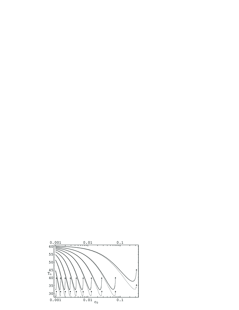
where the coefficients of the inverse metric are and ; the definitions of , , , and can be found in Thorne et al. (1986). The resulting relationship for is shown in Fig. 6 with dashed lines.
For definiteness and simplicity, we assume that the observer is located along the rotation axis of the BH. On its way to the observer, the radiation travels along the null geodesic that originates at a node in the equatorial plane (e.g. , ) and reaches the observer at infinity (, ). Using these as boundary conditions for null geodesics in the Kerr metric (Carter 1968), we numerically find .
Figure 6 shows the dependence of observed time intervals on the value of the speed of sound in the disc. All intervals behave very similarly: they first decrease with increasing and then abruptly increase to infinity due to time dilation. This increase occurs if the innermost node in the pair of nodes comes close to the BH horizon (this is indicated with upward arrows). Although each individual time interval may depend on , the range [, ] of observed time intervals (see the caption to Fig. 6) is independent of for those where there are several peaks observed. With such weak dependence on the speed of sound in the disc, we have only two matching parameters: the specific spin and the mass of the BH.
6.3 Matching the observations
In the flare precursor section we associate the period with the s one (group 5, cf. Table 2 in Aschenbach et al. (2004)) and the time interval with the period of s (group 4 in Aschenbach et al. (2004)). In consistency with the infrared observations of the flare, the periods , , etc. chirp with the peak number (Genzel et al. 2003), i.e. resemble the QPO structure and thus form a cumulative peak of a larger width shifted to higher frequencies on the flares’ power density spectra ( s, group 3, cf. Fig. 3a and 4a in Aschenbach et al. (2004)). We can estimate the average frequency of this peak as .
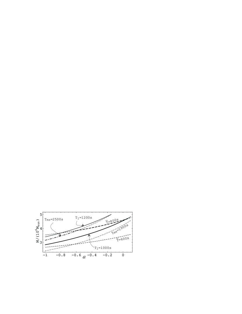
The results of the periods’ matching procedure are shown in Fig. 7. Observational data clearly rules out high positive values of (i.e. the disc orbiting in the same direction as the BH spin), and therefore the accretion disc around the Central Black Hole is likely to be counter-rotating. Moreover, the data presented in Fig. 7 enable us to estimate the mass of the Central Black Hole as . This value is in agreement with the studies by Schödel et al. (2002) and Chez et al. (2003).
7 Conclusions
Allowing for the vertical velocity in the vertical force balance, i.e. performing the two-dimensional analysis, is extremely important, especially near the sonic surface and in the supersonic region. Two-dimensional analysis brings about the existence of the new small radial scale, which is of the order of the thickness of the disc, near the sonic surface. It also shows that the critical condition fixes neither the accretion rate nor the angular momentum of the infalling matter. The nozzle-like shape of the flow around the sonic point leads to the oscillations of disc thickness in the supersonic region that enable us to come up with a straightforward interpretation of quasi-periodical oscillations observed in the radiation coming from the GC (Genzel et al. 2003; Aschenbach et al. 2004). This constrains the mass of the Central Black Hole to which is in agreement with other studies (Schödel et al. 2002; Chez et al. 2003). Our interpretation also suggests that the accretion disc around the Galactic Centre black hole is counter-rotating.
Acknowledgements.
We thank A.V. Gurevich for his interest in the work and for his support, useful discussions and encouragement. We are very grateful to K.A. Postnov for his help and fruitful suggestions regarding the observational part. ADT thanks T. Elmgren for making valuable corrections to the text. This work was supported by the Russian Foundation for Basic Research (grant no. 1603.2003.2), Dynasty fund, and ICFPM.References
- Abramowicz & Zurek (1981) Abramowicz, M. A., Zurek, W. 1981, ApJ, 246, 314
- Abramowicz et al. (1988) Abramowicz, M. A., Czerny, B., Lasota, J.-P., Szuszkiewicz, E. 1988, ApJ, 332, 646
- Abramowicz et al. (1997) Abramowicz, M. A., Lanza, A., & Percival, M. J. 1997, ApJ, 479, 179
- Artemova et al. (2001) Artemova, Yu. V., Bisnovatyi-Kogan, G. S., Igumenshchev, I. V., Novikov, I. D. 2001, ApJ, 549, 1050
- Aschenbach et al. (2004) Aschenbach, B., Grosso, N., Porquet, D., et al. 2004, A&A, 417, 71
- Balbus & Hawley (1998) Balbus, S. A., Hawley, J. F. 1998, Rev. Mod. Phys., 70, 1
- Beloborodov (1998) Beloborodov, A. M. 1998, MNRAS, 297, 739
- Beskin & Pariev (1993) Beskin, V. S., Pariev, V. I., 1993, Phys. Usp., 36, 529
- Beskin (1997) Beskin, V. S. 1997, Phys. Usp., 40, 659
- Beskin et al. (2002) Beskin, V. S., Kompaneetz, R. Yu., & Tchekhovskoy, A. D. 2002, Astron. Lett., 28, 543
- Bondi (1952) Bondi, H. 1952, MNRAS, 112, 195
- Carter (1968) Carter, B. 1968, Phys. Rev., 174, 5
- Chakrabarti (1996) Chakrabarti, S. 1996, ApJ, 471, 237
- Chen et al. (1997) Chen, X., Abramowicz, M. A., & Lasota, J.-P. 1997, ApJ, 476, 61
- Chez et al. (2003) Chez, A. M., Duchêne, G., & Matthews, K., et al. 2003, ApJ, 586, L127
- Frolov & Novikov (1998) Frolov, V. P., Novikov, I. D. 1998, Black Hole Physics. Kluwer Academic Publishers, Dordrecht.
- Gammie & Popham (1998a) Gammie, C. F., Popham, R. 1998a, ApJ, 498, 313
- Gammie & Popham (1998b) Gammie, C. F., Popham, R. 1998b, ApJ, 504, 419
- Genzel et al. (2003) Genzel, R., Schödel, R., & Ott T. et al. 2003, Nature, 425, 934
- Igumenshchev & Beloborodov (1997) Igumenshchev, I. V., Beloborodov, A. M. 1997, MNRAS, 284, 767
- Igumenshchev et al. (2000) Igumenshchev, I. V., Abramowicz, M. A., & Narayan, R. 2000, ApJ, 537, L27
- Krolik & Hawley (2002) Krolik, J. H., Hawley, J. F. 2002, ApJ, 573, 754
- Landau & Lifshits (1987a) Landau, L. D., Lifshits, E. M. 1987a, The Classical Theory of Fields, 4th edn. Butterworth-Heinemann
- Landau & Lifshits (1987b) Landau, L. D., Lifshits, E. M., 1987b, Fluid mechanics, 2nd edn. Butterworth-Heinemann
- Lipunov (1992) Lipunov, V. M. 1992, Astrophysics of Neutron Stars. Springer-Verlag, Berlin
- Lynden-Bell (1969) Lynden-Bell, D. 1969, Nature, 223, 690
- Narayan et al. (1997) Narayan, R., Kato, S., & Honma, F. 1997, ApJ, 476, 49
- Novikov & Thorne (1973) Novikov, I. D., & Thorne, K. S., 1973, in C. DeWitt, B. DeWitt., eds, Black Holes. Gordon and Breach, New York
- Paczyński & Bisnovatyi-Kogan (1981) Paczyński, B., Bisnovatyi-Kogan, G. S. 1981, Acta Astron., 31, 283
- Paczyński & Wiita (1980) Paczyński, B., Wiita, P. J. 1980, A&A, 88, 23
- Papaloizou & Szuszkiewicz (1994) Papaloizou, J., Szuszkiewicz, E. 1994, MNRAS, 268, 29
- Peitz & Appl (1997) Peitz J., Appl S. 1997, MNRAS, 286, 681
- Riffert & Herold (1995) Riffert, H., Herold, H. 1995, ApJ, 450, 508
- Shakura (1972) Shakura, N. I. 1972, AZh, 49, 921
- Shakura & Sunyaev (1973) Shakura, N. I., Sunyaev, R. A. 1973, A&A, 24, 337
- Shapiro & Teukolsky (1983) Shapiro, S. L., Teukolsky, S. A. 1983, Black Holes, White Dwarfs, and Neutron Stars. Wiley–Interscience Publication, New York
- Schödel et al. (2002) Schödel, R., Ott, T., & Genzel, R., et al. 2002, Nature, 419, 664
- Thorne et al. (1986) Thorne, K. S., Price R. N., Macdonald, D. A. 1986, Black Holes: The Membrane Paradigm. Yale Univ. Press, New Haven, CT