XMM-Newton X-ray spectroscopy of the high-mass X-ray binary 4U1700$-$37 at low flux

We present results of a monitoring campaign of the high-mass X-ray binary system 4U~1700$-$37/HD~153919, carried out with XMM-Newton in February 2001. The system was observed at four orbital phase intervals, covering 37% of one 3.41-day orbit. The lightcurve includes strong flares, commonly observed in this source. We focus on three epochs in which the data are not affected by photon pile up: the eclipse, the eclipse egress and a low-flux interval in the lightcurve around orbital phase $\phi\sim 0.25$. The high-energy part of the continuum is modelled as a direct plus a scattered component, each represented by a power law with identical photon index ($\alpha\sim 1.4$), but with different absorption columns. We show that during the low-flux interval the continuum is strongly reduced, probably due to a reduction of the accretion rate onto the compact object. A soft excess is detected in all spectra, consistent with either another continuum component originating in the outskirts of the system or a blend of emission lines. Many fluorescence emission lines from near-neutral species and discrete recombination lines from He- and H-like species are detected during eclipse and egress. The fluorescence Fe K$\alpha$ line at 6.4 keV is very prominent; a second K$\alpha$ line is detected at slightly higher energies (up to 6.7 keV) and a K$\beta$ line at 7.1 keV. In the low-flux interval the Fe K$\alpha$ line at 6.4 keV is strongly (factor $\sim 30$) reduced in strength. In eclipse, the Fe K$\beta$/K$\alpha$ ratio is consistent with a value of 0.13. In egress we initially measure a higher ratio, which can be explained by a shift in energy of the Fe K-edge to $\sim 7.15$ keV, which is consistent with moderately ionised iron, rather than neutral iron, as expected for the stellar wind medium. The detection of recombination lines during eclipse indicates the presence of an extended ionised region surrounding the compact object. The observed increase in strength of some emission lines corresponding to higher values of the ionisation parameter $\xi$ further substantiates this conclusion.

1 Introduction

4U~1700$-$37/HD~153919 is a high-mass X-ray binary (HMXB) discovered by the Uhuru satellite (Jones et al. 1973). HMXBs are relatively young ($<10^{7}$ year) systems composed of a massive OB-type star and a compact object, either a neutron star or a black hole (for a recent catalogue of X-ray binaries see Liu et al. 2000). X-rays are produced when matter from the OB star accretes onto the compact object. The majority ($\sim 80\%$) of the HMXBs are Be/X-ray binaries. These systems are often X-ray transients, only producing X-rays when the compact object accretes matter by passing through the dense equatorial disc of a Be-star. The other group of systems host a more massive OB supergiant (for a review see Kaper 2001). About a dozen OB supergiant X-ray binary systems are known in the Milky Way and the Magellanic Clouds. Among them are a few that host a black-hole candidate (e.g. Cyg~X$-$1).

Accretion takes place through either the strong stellar wind of the optical companion or Roche-lobe overflow. In a wind-fed system the X-rays ionise a relatively small region in the stellar wind due to the low X-ray luminosity (L_X $\sim 10^{35}-10^{36}$ erg s^-1). The size of the ionisation zone can be determined from the orbital modulation of UV resonance lines formed in the wind (Hatchett & McCray 1977; van Loon et al. 2001). In a Roche-lobe overflow system, matter flows via the inner Lagrangian point to an accretion disc. A powerful X-ray source (L_X $\sim 10^{38}$ erg s^-1) is produced, which ionises almost the whole stellar wind, such that only in the X-ray shadow of the optical companion a stellar wind can emerge (e.g. LMC~X$-$4; Boroson et al. 1999). For a more general review on X-ray binaries we refer to e.g. Nagase (1989) or Lewin et al. (1995).

X-ray spectra of HMXBs are often described by a power law with photon index $\alpha\sim 1$, modified at high energies (above 10–20 keV) by an exponential cutoff. A spectrum of this form can be produced by inverse Compton scattering of soft X-rays by hot electrons in the accretion column near the compact object (e.g. Hayakawa 1985). This continuum component is often scattered by the stellar wind of the optical companion. This results in a similar component, but with a different absorption column depending on the orbital phase of the system. In the high energy part ($\gtrsim 10$ keV) of the spectrum of most X-ray pulsars broad absorption lines have been discovered, which are attributed to cyclotron resonant scattering. From the energy of these lines strong magnetic fields are inferred ($B\sim 10^{12}$ Gauss; e.g. Trümper et al. 1978).

In some HMXBs a soft excess at $\sim 0.1-1$ keV is detected of which the physical origin is not well understood. If this component has a thermal origin, its relatively low temperature requires in some cases a size of the emission region much larger than the size of the compact object, of the order of the magnetospheric radius, where the pressure of the infalling matter balances the pressure of the magnetic field of the compact object (e.g. Cen~X$-$3; Burderi et al. 2000). Hickox et al. (2004) show that a soft excess is very common in X-ray binary pulsars and that observations that do not show evidence of a soft excess are probably limited by high absorption, low flux or insufficient soft sensitivity. Hickox et al. (2004) find that the soft excess in luminous (L_X $\gtrsim 10^{38}$ erg s^-1) sources can be explained by repocessing of hard X-rays from the neutron star by optically thick, accreting material. For less luminous (L_X $\lesssim 10^{36}$ erg s^-1) sources the soft excess is probably due to other processes, e.g. emission from photoionised or collisionally heated diffuse gas or thermal emission from the surface of the neutron star.

With the advent of the X-ray observatories Chandra and XMM-Newton it has become possible to study the X-ray spectra of HMXBs in unprecedented detail. Their eclipse spectra show many emission lines and radiative recombination continua (e.g. Vela~X$-$1 Schulz et al. 2002; Goldstein et al. 2004). Such an emission line spectrum originates in the ionisation zone surrounding the X-ray source and becomes detectable during eclipse due to the supression of the strong continuum emission produced by the X-ray pulsar. Paerels et al. (2000) show that the Chandra spectrum of Cyg~X$-$3 is consistent with a cool, optically thin, photoionised plasma in equilibrium, whereas the spectrum of 4U~1700$-$37 shows a more “hybrid” plasma in which also evidence is found for a collisionally ionised plasma (Boroson et al. 2003). Wojdowski et al. (2003) report on an apparent change of plasma properties from eclipse to eclipse egress of Cen~X$-$3, which they can explain with a photoionised plasma for which the effects of resonant line scattering are taken into account as well. Watanabe et al. (2003) report on a fully resolved Compton-scattered Fe K$\alpha$ fluorescence line in GX~301$-$2. They show that the flux ratio of the line and shoulder together with the energy distribution of the shoulder can be used to directly constrain the absorption column, temperature and abundances of the scattering medium.

1.1 4U 1700$-$37

Located at a distance of 1.9 kpc (Ankay et al. 2001) 4U~1700$-$37 is powered by the dense stellar wind (Ṁ$\sim 10^{-5}$ M_⊙ yr^-1; Clark et al. 2002) of the O6.5 Iaf+ supergiant HD~153919 (Jones et al. 1973; Mason et al. 1976). It is the hottest and most luminous optical companion known in HMXBs. Ankay et al. (2001) propose that the system escaped the OB association Sco OB1 $\sim$ 2 million years ago, travelling with a velocity of $\sim$ 75 km s^-1. They show that the progenitor of the compact object should have evolved into a supernova within $\sim$ 6 million years (if it was born as a member of the association). This corresponds to a lower limit of its initial mass of $\sim$ 30 M_☉ (Schaller et al. 1992).

Periodic X-ray pulsations have not been detected so far (although Boroson et al. 2003 report quasi-periodic oscillations), so that the nature of the compact object remains unclear (Gottwald et al. 1986; Clark et al. 2002). Most likely, 4U~1700$-$37 is a neutron star since its X-ray spectrum is well described by the standard accreting pulsar model (White et al. 1983). There are indications that the mass of the compact object is larger than 2 M_☉ (Rubin et al. 1996; Clark et al. 2002). If true, this might qualify it as a low-mass black-hole (Brown et al. 1996) or a massive neutron star, like in Vela~X$-$1 (Barziv et al. 2001; Quaintrell et al. 2003). Reynolds et al. (1999) report the possible presence of a cyclotron feature at $\sim 37$ keV in BeppoSAX observations. If real, 4U~1700$-$37 has a magnetic field $B\sim 2.3\times 10^{12}$ Gauss, characteristic of a HMXB accreting pulsar.

This system is unique in showing broad and variable emission lines in the ultraviolet part of the spectrum. Kaper et al. (1990) propose that these lines are produced by photons from strong EUV emission lines close to the He ii Lyman-$\beta$ transition (256 Å), which are Raman scattered by He ii ions in the stellar wind of the optical companion via the corresponding downwards transition near the He ii Balmer-$\alpha$ line at 1640 Å. The input EUV emission lines can not be studied directly due to the opaqueness of the interstellar medium. However, Kaper et al. (1990) show that these emission lines originate close to the compact object, causing the orbital modulation of the Raman scattered lines. Although the central wavelength of the input EUV emission lines is known, they could not be identified due to the multitude of candidate line features in this part of the spectrum.

The X-ray spectrum of 4U~1700$-$37 can be modelled as a power law with a high-energy cutoff (Haberl et al. 1989; Reynolds et al. 1999), modified by an absorption column which depends on the orbital phase of the system. A sharp increase in absorption at late orbital phases (Mason et al. 1976; Haberl et al. 1989) is explained by the presence of a region of enhanced density trailing the compact object in its orbit, such as a photo-ionisation wake (Blondin et al. 1990). The presence of such a wake in 4U~1700$-$37 has been confirmed with optical spectroscopy (Kaper et al. 1994). A similar increase in absorption has been reported for other HMXBs, like Vela~X$-$1 and Cen~X$-$3 (Haberl & White 1990; Nagase et al. 1992).

Figure 1: 0.3–11.5 keV lightcurve of 4U 1700$-$37 obtained with the EPIC/MOS-2 camera at the end of February 2001 in four orbital phase intervals. The data have been extracted from a circular region centered on the source and binned in time-bins of 10 seconds. The data have not been corrected for pile-up, which mainly distorts the shape of the spectrum but may also affect the value of the high count rates, e.g. during flares. We selected three intervals in the lightcurve (indicated by the vertical dashed lines), in which the spectrum does not suffer from pile-up, i.e. the eclipse, the eclipse egress and a low-flux interval, centered on orbital phase $\phi\sim 0.25$.

A soft excess was found in Ginga observations (Haberl & Day 1992) and modelled as a bremsstrahlung component with a temperature of kT $\sim 0.5$ keV. In a second set of Ginga observations Haberl et al. (1994) also found a difference in temperature before and after eclipse, which they tentatively explain with a bow shock in front of the compact object, heating the stellar wind to a higher temperature.

Boroson et al. (2003) obtained Chandra observations of 4U~1700$-$37 in August 2000 in the orbital phase interval $0.65\leq\phi\leq 0.8$. They find emission lines in the 4–13 Å range, which are identified with fluorescence emission lines from near-neutral species and recombination lines from He- and H-like species. The X-ray source was observed during an intermittent flaring state, in which the strengths of the lines vary. The triplet structure of Si xiii and Mg xi is resolved but weak, but could be used to tentatively identify the plasma as a low-density hybrid of a photo-ionised and a collisionally ionised plasma (Boroson et al. 2003).

We monitored 4U~1700$-$37 with XMM-Newton around the four quadratures in the orbit, including part of the eclipse and the eclipse egress. The goal of our observing campaign is to study the X-ray spectrum as a function of orbital phase and to derive information on the physical origin of the continuum and line emission. In Sect. 2 we describe the observations and the techniques that we used to reduce the dataset; in Sect. 3 we present the spectral analysis, and in Sect. 4 we discuss our results.

Table 1: Log of XMM-Newton observations of 4U 1700$-$37 in the period 17–20 February 2001. To calculate the orbital phase we used the ephemeris of Rubin et al. (1996): orbital period P_orb = 3.411581(27) d and mid-eclipse T₀ = JD 2448900.873(2).

Tstart	Tend	$\Delta t$	$\Delta\phi$
(MJD)	(MJD)	(ks)
51957.863	51958.166	25.79	0.22 - 0.31
51958.729	51959.106	32.87	0.48 - 0.59
51959.577	51959.813	20.90	0.72 - 0.79
51960.745	51961.104	31.36	0.07 - 0.17

2 Observations

We have obtained four 20–30 ks observations of 4U~1700$-$37 with XMM-Newton (Jansen et al. 2001) in the period 2001, February 17–20. The log of observations is listed in Table 1. Fig. 1 shows the lightcurve of the four intervals obtained with EPIC/MOS-2 (Turner et al. 2001). To determine the orbital phase we used the ephemeris of Rubin et al. (1996). The X-ray flux of 4U1700$-$37 is strongly variable (factor $\sim 10$). Numerous flares are observed with a typical duration of the order of half an hour.

Due to the brightness of the optical companion (M${}_{\rm V}=6.5$), we were forced to switch off the Optical Monitor. The EPIC/MOS-1 and EPIC/PN detectors (Strüder et al. 2001) were used in timing and burst mode, respectively, to cope with the high count rate of the X-ray source. EPIC/MOS-2 was used in small-window mode. For the RGS gratings (den Herder et al. 2001) default settings were used.

We reduced the data using the Science Analysis System (SAS) version 5.3.3. Since this version does not yet contain a developed task to reduce EPIC/MOS-1 timing and EPIC/PN burst mode, in this paper we will concentrate on the EPIC/MOS-2 and RGS datasets. The results from the EPIC/PN and EPIC/MOS-1 will be reported in a forthcoming paper.

Since the pipeline products were created when the reduction software was still in an early stage, we created new event lists for the EPIC/MOS-2 data. These event lists were filtered following the data analysis threads provided by the XMM-Newton team. Because the instrument was set in small-window mode (to reduce the read-out time) our strong source produced numerous events over almost the whole frame, which prevented us from measuring the background. Therefore, we extracted a background spectrum using special event lists provided by the XMM-Newton team. These are long exposure observations of fields with a typical background and without any bright sources. Since our source is bright, the background contribution is negligible ($\sim 0.1\%$ in the energy range 0.3–11.5 keV and $\lesssim 2\%$ in the energy range 0.3–2.0 keV).

Figure 2: XMM/EPIC observation of 4U 1700$-$37 during eclipse egress ($0.14\leq\phi\leq 0.17$). The continuum emission is modelled as three power laws, representing a direct (solid line), a scattered (dashed-dotted line) and a soft component (dotted line). The spectrum clearly shows several fluorescence emission lines and some discrete recombination lines of He- and H-like species (see Table 3 for their identification). Note that the data in this plot are folded with the response matrix of the instrument. Therefore, some of the features (e.g. at 1.8 keV) in the plot are of instrumental origin. The lower panel shows the residuals of the model to the spectrum.

Due to the high count rate a large fraction of the dataset is affected by pile-up. The basic concept of pile-up is that a saturation effect takes place in which two or more separate photons fall onto the same pixel within a read-out cycle and are counted as one with a total energy equal to the sum of their energies (for a detailed description see e.g. Ballet 1999). This effect distorts the source spectrum and the measured flux. The SAS software provides the tool EPATPLOT to analyse the distribution of patterns produced on the CCDs by the incoming photons. Two or more photons counted as one have a lower probability to produce a single-pixel pattern than one photon with the same energy. This affects the observed pattern distribution, which can be compared with the expected distribution to assess the pile-up. However, with this method it is not clear to what extent the spectral parameters (derived from fits to the extracted spectrum) are affected by pile-up.

In order to assess the magnitude of the distortion and to eliminate the part of the point spread function (PSF) affected by pile-up, we created multiple event lists, extracted from annuli centered on the source, with increasing inner radii (with steps of $2.5\arcsec$) up to a maximum of $25\arcsec$. We modelled the spectra with the same basic model of two absorbed power laws (see Sect. 3.1). The best-fitted spectral parameters were then examined as a function of inner radius of the extraction region. One expects the parameters to stabilise beyond the radius at which pile-up no longer affects the remaining part of the PSF. However, we find that the parameters continue changing, sometimes even up to the maximum inner radius, while EPATPLOT already gives satisfactory results. We conclude that the model of the energy dependence of the PSF is not known accurately enough for our purpose.

In the current study we concentrate on data with a sufficiently low countrate. We select three intervals in the lightcurve (see Fig. 1): eclipse, eclipse egress and a low-flux part centered on orbital phase $\phi\sim 0.25$. These intervals of low flux are not uncommon in 4U~1700$-$37 (e.g. Boroson et al. 2003) and are also observed in other HMXBs, e.g. 4U~1907$+$097 studied by in ’t Zand et al. (1997), who refer to this behaviour as “dipping activity”.

We also analysed the RGS data extracted in the same timeframes. However, the source is highly absorbed, resulting in a very low RGS-countrate. After rebinning the data to 20-25 counts per bin the RGS spectra were used to verify the best-fit models for the EPIC/MOS-2 data.

3 Spectral Analysis

The EPIC/MOS-2 camera covers the energy range 0.3–11.5 keV. In previous studies based on a wider energy range (EXOSAT, 3–20 keV, Haberl et al. 1989; BeppoSAX, 0.5–200 keV, Reynolds et al. 1999) the continuum of 4U~1700$-$37 is modelled as an absorbed power law with photon index $\alpha$, modified above a break energy $E_{c}$ by a high-energy cutoff of the form $\exp{\left[(E_{c}-E)/E_{f}\right]}$.

Figure 3: XMM/EPIC observation of the 4U 1700$-$37 during the low-flux interval. A soft excess below $\sim 2$ keV is clearly present. The solid line represents a model that consists of one absorbed power-law component. The lower panel shows the residuals of the model to the spectrum.

Sako et al. (1999) obtain a good fit of the ASCA eclipse spectrum of Vela~X$-$1 using two absorbed power laws with identical photon index, but different column density $N_{H}$ and normalisation to model the continuum. One power law describes the direct component, that originates from close to the neutron star. A part of this component is scattered by the extended stellar wind of the optical companion and is described by the second powerlaw. Boroson et al. (2003) apply the same method to fit the Chandra spectrum of 4U~1700$-$37. We follow the same strategy modelling the XMM-Newton spectra. We apply three models to fit the continuum at eclipse, egress and low flux. The emission lines are subsequently fit by gaussians. The spectra have been analysed using XSPEC version 11.2.0, after rebinning the spectra to 25 counts per bin.

3.1 Continuum Emission

We first describe the eclipse egress spectrum, where a clear distinction can be made between the different continuum components (see Fig. 2). We discuss the high-energy and the low-energy part of the spectra separately. Note that the mentioned parameters correspond to the models fitted to the full 0.3–11.5 keV energy range. Table 2 lists the models we used to fit these three spectra of which the parameters are constrained: model A, which consists of three power laws, model B with two (or three) power laws modified by a high-energy cutoff, and model C, similar to model A, but with a blackbody component replacing the power law describing the soft component.

3.1.1 Direct and scattered component

We model the high energy part of the eclipse egress spectrum as two power laws, each of them modified by different absorbing columns (Morrison & McCammon 1983) depending on the orbital phase of the system (for the egress spectrum these are N${}_{\rm H}\sim 8.3\times 10^{23}$ cm^-2 and N${}_{\rm H}\sim 1.8\times 10^{23}$ cm^-2; see model A in Table 2). Both components have the same power law index $\alpha\sim 1.4$. The hard, direct component is assumed to originate from the near surroundings of the compact object and the scattered component is produced by Thomson scattering by electrons in the extended stellar wind of the optical companion. Since Thomson scattering is energy independent, the photon index of the scattered component is expected to be the same, and is therefore fixed to the index of the direct component. The best-fit values of the model parameters are given in Table 2. Both components are also detected during the part of the eclipse covered by our observations ($0.07\leq\phi\leq 0.14$), although the flux of the direct component is reduced by a factor $\sim 45$ compared to egress.

Table 2: Parameters used to describe the continuum models of the eclipse egress, eclipse and low-flux spectra. All errors and upper limits are a 1 $\sigma$ confidence level. Three different models are considered. Model A consists of three power-law components with identical photon index, but different normalisation, which are modified by different absorption columns. Model B contains two power-law components, modified by a high-energy cutoff. Model C includes a blackbody component replacing one of the three power-law components of model A.

	egress			eclipse			low-flux
	Model A	Model B	Model C	Model A	Model B	Model C	Model A	Model B	Model C
direct component
NH ($\times 10^{22}$ cm-2)	$83\pm 2$	$85\pm 3$	$83\pm 2$	$59\pm 8$	$89\pm 12$	$61\pm 9$	$20\pm 3$	$6.8\pm 0.4$	$17\pm 2$
Normalisation ($\times 10^{-2}$ photons s-1 cm-2 keV-1 at 1 keV)	$44\pm 6$	$12\pm 2$	$44\pm 6$	$1.1\pm 0.4$	$0.47\pm 0.19$	$1.1_{-0.3}^{+0.6}$	$8.7\pm 2.4$	$3.8\pm 0.6$	$9.3\pm 2.0$
Unabsorbed flux ($\times 10^{-10}$ erg s-1 cm-2)	$49\pm 3$	$34\pm 5$	$49\pm 3$	$1.1\pm 0.3$	$1.0\pm 0.4$	$1.2\pm 0.4$	$5.3_{-0.7}^{+1.5}$	$5.3\pm 1.0$	$6.1\pm 1.0$
scattered component
NH ($\times 10^{22}$ cm-2)	$17.5\pm 1.3$	$18.7\pm 1.6$	$17.6\pm 2.2$	$11.6\pm 0.7$	$11.2\pm 0.7$	$12.3\pm 1.0$	$7.2\pm 0.3$	$...$	$6.4\pm 0.4$
Normalisation ($\times 10^{-2}$ photons s-1 cm-2 keV-1 at 1 keV)	$1.6\pm 0.3$	$0.67\pm 0.13$	$1.6\pm 0.4$	$0.56\pm 0.12$	$0.24\pm 0.05$	$0.61\pm 0.15$	$8.2\pm 1.4$	$...$	$6.3\pm 1.4$
Unabsorbed flux ($\times 10^{-10}$ erg s-1 cm-2)	$1.7\pm 0.2$	$1.9\pm 0.4$	$1.8\pm 0.3$	$0.60\pm 0.06$	$0.54\pm 0.12$	$0.66\pm 0.07$	$5.3\pm 0.7$	$...$	$4.1\pm 0.7$
soft component
NH ($\times 10^{22}$ cm-2)	$0.56\pm 0.09$	$0.36\pm 0.08$	$0.30\pm 0.17$	$0.24\pm 0.04$	$0.13\pm 0.04$	$<0.05$	$0.43\pm 0.08$	$0.32\pm 0.07$	$1.0\pm 0.4$
Normalisation ($\times 10^{-4}$ photons s-1 cm-2 keV-1 at 1 keV)	$4.3\pm 0.5$	$2.6\pm 0.3$	$...$	$2.3\pm 0.2$	$1.7\pm 0.2$	$...$	$4.7\pm 0.9$	$3.4\pm 0.7$	$...$
Blackbody temperature (keV)	$...$	$...$	$0.74_{-0.19}^{+0.34}$	$...$	$...$	$0.77_{-0.03}^{+0.11}$	$...$	$...$	$0.13\pm 0.04$
Normalisation ($\times 10^{32}$ erg s-1 kpc-2)	$...$	$...$	$2.1_{-0.5}^{+1.7}$	$...$	$...$	$1.3\pm 0.4$	$...$	$...$	$<270$
Unabsorbed flux ($\times 10^{-12}$ erg s-1 cm-2)	$4.7\pm 0.5$	$7.5\pm 0.8$	$1.8_{-0.4}^{+1.4}$	$2.5\pm 0.3$	$3.7\pm 0.4$	$1.1\pm 0.3$	$3.0\pm 0.5$	$4.7\pm 1.1$	$<230$
Cutoff energy (keV)	$...$	$5.4$ fixed	$...$	$...$	$5.4$ fixed	$...$	$...$	$5.4\pm 0.4$	$...$
Folding energy (keV)	$...$	$10.6$ fixed	$...$	$...$	$10.6$ fixed	$...$	$...$	$10.6_{-1.6}^{+2.3}$	$...$
Photon index	$1.35\pm 0.05$	$0.61\pm 0.05$	$1.35\pm 0.05$	$1.36\pm 0.12$	$0.77\pm 0.12$	$1.37\pm 0.13$	$1.87_{-0.04}^{+0.09}$	$1.08\pm 0.09$	$1.83\pm 0.08$
$\chi^{2}/\rm{d.o.f}$	$558/522$	$578/522$	$559/521$	$444/408$	$445/408$	$443/407$	$485/390$	$487/390$	$475/389$

In the low-flux spectrum it is difficult to separate the two components. The model produces comparable strengths and absorption coefficients (Model A in Table 2) with a photon index that is slightly higher ($\alpha\sim 1.9$) than in eclipse and egress. Modelling the spectrum with only one power law modified by a high-energy cutoff gives an equally good fit (model B in Table 2). The resulting photon index is lower ($\alpha\sim 1.1$) than in model A. The cutoff energy in this model is $\sim 5.4$ keV (see Table 2), which is in agreement with previous observations (e.g. Haberl et al. 1989, who find $E_{c}=6.6\pm 0.7$ keV in EXOSAT observations and Reynolds et al. 1999 who find $E_{c}=5.9\pm 0.2$ keV in BeppoSAX observations). However, the folding energy we find ($E_{f}\sim 11$ keV) is low; Haberl et al. (1989) find $E_{f}=21\pm 4$ keV and Reynolds et al. (1999) measure $E_{f}=23.9\pm 0.9$ keV.

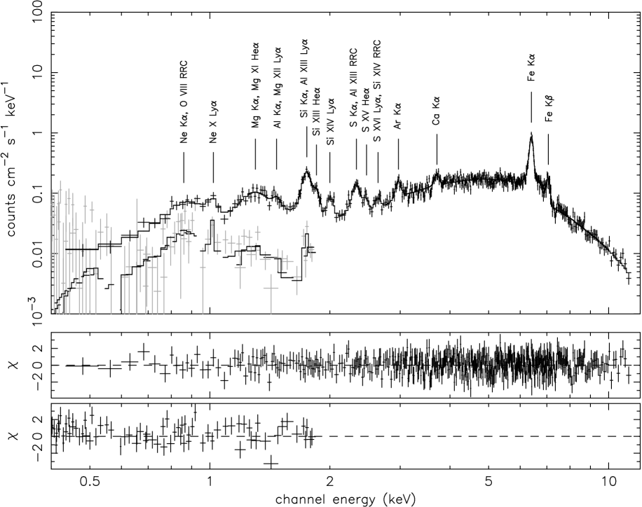
Figure 4: XMM/EPIC observation of 4U 1700$-$37 during eclipse. The spectrum clearly shows several fluorescence emission lines and some discrete recombination lines of He- and H-like species with their identifications. The continuum model used for this spectrum is model A (see Table 2); the RGS spectrum is also included. The EPIC/MOS-2 residuals are shown in the middle panel, and the RGS residuals in the lower panel.

The problem with applying this model to our dataset is that the folding energy is outside the energy range of EPIC/MOS-2 (0.3–11.5 keV) and its value is easily influenced by the value of the photon index. If we apply the model to the eclipse and egress spectrum, a high-energy cutoff yields an unacceptable fit, and the fit parameters can not be constrained. If we fix E_c and E_f to the values obtained from the low-flux spectrum, the fit parameters can be constrained (see Table 2). This is also the case if we fix their values to the values of the BeppoSAX observations (Reynolds et al. 1999). The fits with model A and with this “fixed” version of model B are of comparable quality for the eclipse spectrum, but for egress fits with model B are worse than fits with model A ($\chi^{2}/{\rm d.o.f.}=578/522$ for model B compared to $558/522$ for model A; d.o.f. = degrees of freedom). Note that model B also indicates a higher photon index in the low-flux interval compared to eclipse and egress.

3.1.2 Soft Excess

After having obtained the best fit for the models discussed above, an excess remains in all cases in the low energy part of the spectrum (see Fig. 3). A soft excess is reported for many X-ray spectra of HMXBs, but the nature of this component is not clear. To investigate the physical origin of this component we fit the soft component with four different models, which are discussed below: bremsstrahlung, blackbody, electron scattering and dust scattering. In all cases it is found that the model component needs to be modified by a moderate absorption column, close to the interstellar value N${}_{\rm H}\sim 0.3\times 10^{22}$ cm^-2 for this source, based on the observed reddening $\rm E(B-V)=0.59$ (Hutchings et al. 1973) and N${}_{\rm H}\rm/E(B-V)=0.58\times 10^{22}$ cm^-2 mag^-1 (Kilian 1992).

Adding a bremsstrahlung component, as proposed by Haberl & Day (1992) and Haberl et al. (1994), improves the fit to all three spectra significantly ($\chi^{2}/{\rm d.o.f.}=476/389$ for the low-flux spectrum). However, the temperature of the bremsstrahlung component can not be constrained in any of the spectra. Actually, this bremsstrahlung component tends to mimic the shape of a power law. This suggests that bremsstrahlung is not the physical origin of the soft excess.

Fitting this excess with a blackbody component gives a similar improvement of the fit ($\chi^{2}/{\rm d.o.f.}=475/389$ for the low-flux spectrum). For this model the temperature $\rm kT\sim 0.13$ keV. The flux is not constrained in the low-flux spectrum, but we can place an upper limit of $2.3\times 10^{-10}$ erg s^-1 cm^-2. In the eclipse and egress spectra the resulting temperature is slightly higher ($\rm kT\sim 0.77$ keV and $\rm kT\sim 0.74$ keV, respectively). The unabsorbed flux is constrained to $1.1\times 10^{-12}$ erg s^-1 cm^-2 and $1.8\times 10^{-12}$ erg s^-1 cm^-2, respectively (see model C in Table 2).

Modelling the soft excess with yet another (third) power law with a photon index fixed to that of the direct and scattered component also gives a significant improvement ($\chi^{2}/{\rm d.o.f.}=485/390$) and all the parameters are constrained (see Table 2). This component could, like the scattered component of model A, represent a Thomson scattered version of the hard, direct component, with a very low absorption column (N${}_{\rm H}\sim 0.43\times 10^{22}$ cm^-2).

Table 3: List of the emission lines that have been detected in the eclipse, the eclipse-egress and the low flux spectra. All errors and upper limits are 1 $\sigma$. If a line is detected in one spectrum but not in another, an upper limit on the flux is given.

	eclipse	egress	low-flux		eclipse	egress	low-flux
Energy (keV)	$0.86\pm 0.02$	$0.87\pm 0.02$	$0.86\pm 0.02$		$2.46\pm 0.01$	$2.42_{-0.02}^{+0.04}$	$2.46$ fixed
Width (eV)	$71\pm 19$	$84\pm 32$	$60\pm 27$		$<18$	$115\pm 29$	$20$ fixed
Flux ($10^{-5}$ photons cm-2 s-1)	$4.0\pm 1.0$	$5.5\pm 2.0$	$5.3\pm 1.8$		$1.6\pm 0.4$	$9.8\pm 2.9$	$<6.1$
Identification	${Ne\leavevmode\nobreak\ K\alpha\textsc{}},\leavevmode\nobreak\ {O\textsc{viii}}\leavevmode\nobreak\ {\rm RRC}$				${S\textsc{xv}}\leavevmode\nobreak\ {\rm He\alpha}$
Energy (keV)	$1.01\pm 0.01$	$1.01$ fixed	$1.01$ fixed		$2.63\pm 0.01$	$2.63$ fixed	$2.63$ fixed
Width (eV)	$<13$	$13$ fixed	$13$ fixed		$<27$	$27$ fixed	$27$ fixed
Flux ($10^{-5}$ photons cm-2 s-1)	$1.0\pm 0.3$	$<0.52$	$<1.7$		$1.1\pm 0.3$	$<1.8$	$<2.0$
Identification	${Ne\textsc{x}}\leavevmode\nobreak\ {\rm Ly\alpha}$				${S\textsc{xvi}}\leavevmode\nobreak\ {\rm Ly\alpha},\leavevmode\nobreak\ {Si\textsc{xiv}}\leavevmode\nobreak\ {\rm RRC}$
Energy (keV)	$1.30\pm 0.01$	$1.32\pm 0.03$	$1.31$ fixed		$2.97\pm 0.01$	$2.96\pm 0.01$	$2.97$ fixed
Width (eV)	$77\pm 17$	$<87$	$87$ fixed		$<29$	$<38$	$29$ fixed
Flux ($10^{-5}$ photons cm-2 s-1)	$3.1\pm 0.7$	$2.2\pm 0.7$	$<3.3$		$2.8\pm 0.4$	$4.7\pm 0.9$	$<4.6$
Identification	${Mg\leavevmode\nobreak\ K\alpha\textsc{}},\leavevmode\nobreak\ {Mg\textsc{xi}}\leavevmode\nobreak\ {\rm He\alpha}$				${Ar\leavevmode\nobreak\ K\alpha\textsc{}}$
Energy (keV)	$1.47\pm 0.02$	$1.47$ fixed	$1.47$ fixed		$3.14$ fixed	$3.14\pm 0.02$	$3.14$ fixed
Width (eV)	$<31$	$31$ fixed	$31$ fixed		$56$ fixed	$56\pm 32$	$56$ fixed
Flux ($10^{-5}$ photons cm-2 s-1)	$0.6\pm 0.2$	$<0.78$	$<0.15$		$<0.69$	$4.3\pm 1.4$	$<0.81$
Identification	${Al\leavevmode\nobreak\ K\alpha\textsc{}},\leavevmode\nobreak\ {Mg\textsc{xii}}\leavevmode\nobreak\ {\rm Ly\alpha}$				${Ar\textsc{xvii}}\leavevmode\nobreak\ {\rm He\alpha}$
Energy (keV)	$1.75\pm 0.01$	$1.77\pm 0.01$	$1.76$ fixed		$3.71\pm 0.01$	$3.75\pm 0.02$	$3.71$ fixed
Width (eV)	$<26$	$<26$	$26$ fixed		$<28$	$<46$	$30$ fixed
Flux ($10^{-5}$ photons cm-2 s-1)	$5.0\pm 0.6$	$4.8\pm 0.9$	$<0.35$		$2.7\pm 0.5$	$3.4\pm 1.1$	$<6.3$
Identification	${Si\leavevmode\nobreak\ K\alpha\textsc{}},\leavevmode\nobreak\ {Al\textsc{xiii}}\leavevmode\nobreak\ {\rm Ly\alpha}$				${Ca\leavevmode\nobreak\ K\alpha\textsc{}}$
Energy (keV)	$1.85\pm 0.01$	$1.86\pm 0.06$	$1.83\pm 0.03$		$6.40\pm 0.01$	$6.42\pm 0.01$	$6.41_{-0.04}^{+0.05}$
Width (eV)	$<20$	$<101$	$<42$		$<15$	$22\pm 10$	$<65$
Flux ($10^{-5}$ photons cm-2 s-1)	$3.4\pm 0.8$	$1.6_{-0.9}^{+1.6}$	$2.7\pm 1.5$		$62.5\pm 1.9$	$150\pm 7$	$5.3_{-2.1}^{+7.3}$
Identification	${Si\textsc{xiii}}\leavevmode\nobreak\ {\rm He\alpha}$				${Fe\leavevmode\nobreak\ K\alpha\textsc{i-xvii}}$
Energy (keV)	$2.00\pm 0.01$	$2.02\pm 0.01$	$2.01$ fixed		$6.53\pm 0.04$	$6.72\pm 0.02$	$6.72$ fixed
Width (eV)	$<18$	$<31$	$20$ fixed		$206\pm 30$	$<42$	$42$ fixed
Flux ($10^{-5}$ photons cm-2 s-1)	$1.6\pm 0.3$	$1.9\pm 0.5$	$<4.2$		$19.2\pm 2.9$	$20\pm 5$	$<0.92$
Identification	${Si\textsc{xiv}}\leavevmode\nobreak\ {\rm Ly\alpha}$				${Fe\leavevmode\nobreak\ K\alpha\textsc{xviii-xxiv}},\leavevmode\nobreak\ {Fe\textsc{xxv}}\leavevmode\nobreak\ {\rm He\alpha}$
Energy (keV)	$2.33\pm 0.01$	$2.32\pm 0.01$	$2.33$ fixed		$7.06\pm 0.01$	$7.11\pm 0.01$	$7.06$ fixed
Width (eV)	$34\pm 11$	$<34$	$34$ fixed		$<28$	$37\pm 25$	$28$ fixed
Flux ($10^{-5}$ photons cm-2 s-1)	$6.3\pm 0.7$	$6.1\pm 1.4$	$<4.9$		$11.3\pm 1.1$	$60\pm 7$	$<13.1$
Identification	${S\leavevmode\nobreak\ K\alpha\textsc{}},\leavevmode\nobreak\ {Al\textsc{xiii}}\leavevmode\nobreak\ {\rm RRC}$				${Fe\leavevmode\nobreak\ K\beta\textsc{i-xvii}}$

Scattering by dust grains becomes a possibility at larger distance from the system (where the absorption is low) as found by Ebisawa et al. (1996) in the ASCA observations of Cen~X$-$3. We add 2 to the photon index of the soft component compared to the index of the hard component, since dust scattering, unlike Thomson scattering, is energy dependent ($\propto 1/E^{2}$). This model results in an equally good fit as Thomson scattering for the low-flux and egress spectrum. Since the difference between Thomson scattering and dust scattering in our models is produced by a change in the photon index, this will only be visible as a difference in flux at the high energy part of the spectrum. However, this part of the spectrum is dominated by the flux of the direct component and therefore the difference between dust or Thomson scattering is difficult to measure. For the eclipse spectrum, where the direct component does not dominate the high-energy part of the spectrum, the dust scattering model yields a significantly worse fit ($\chi^{2}/{\rm d.o.f.}=453/408$) than Thomson scattering ($\chi^{2}/{\rm d.o.f.}=444/408$).

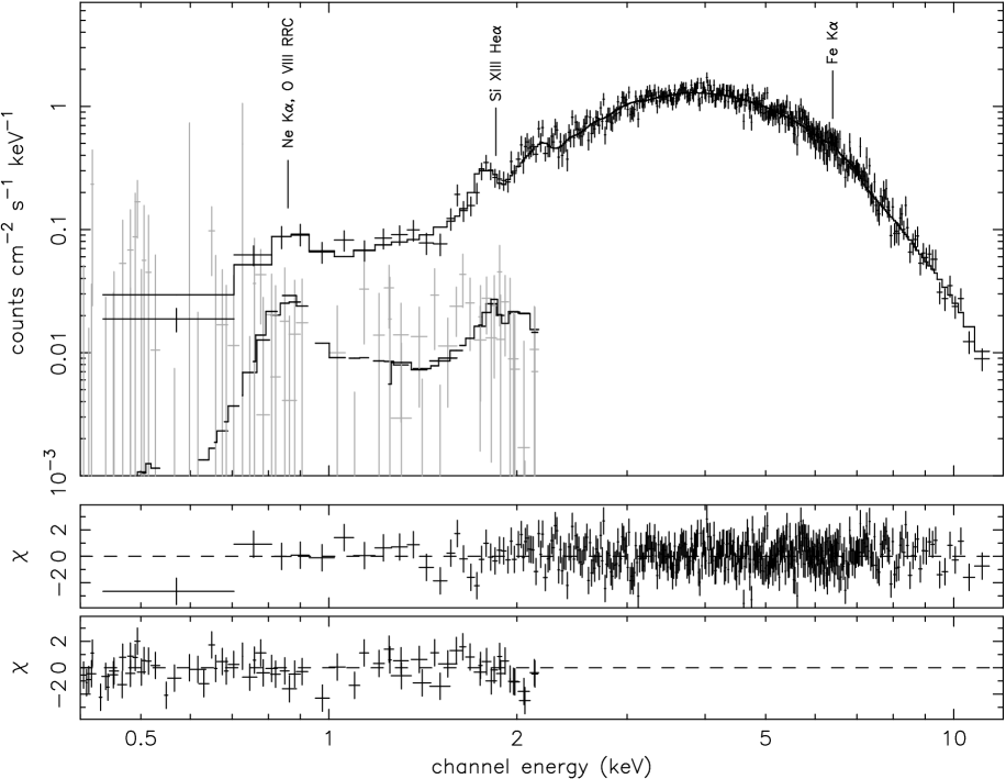
Figure 5: XMM/EPIC observation of the 4U 1700$-$37 during low flux. The soft excess has been fit by a third power-law component. Only some of the many lines observed in eclipse and egress are detected. Especially the strong reduction of the iron complex is remarkable. The RGS spectrum is displayed in the left bottom corner of the upper panel. The EPIC/MOS-2 residuals are shown in the middle panel, and the RGS residuals in the lower panel.

Following the approach of Boroson et al. (2003) we also try to model the soft excess as a blend of gaussians only. We delete the soft continuum component from model A and refit the data. At low energies the fit now contains broad lines with a width on the order of 150–180 eV, whereas the resolution of EPIC/MOS-2 has a width of $\sim 40$ eV at 1 keV. The absorption of the direct and scattered components is “lower” in eclipse than in egress (N${}_{\rm H}\sim 5.6\times 10^{22}$ cm^-2 and N${}_{\rm H}\sim 30\times 10^{22}$ cm^-2 in eclipse w.r.t N${}_{\rm H}\sim 15.3\times 10^{22}$ cm^-2 and N${}_{\rm H}\sim 82\times 10^{22}$ cm^-2).

We also investigated the soft component in the RGS dataset (see Fig. 5). Due to the low RGS count rate it was not possible to set further constraints.

3.2 Line Emission

As in other HMXBs (e.g. Vela~X$-$1 and Cen~X$-$3; Sako et al. 1999; Ebisawa et al. 1996), 4U~1700$-$37 shows many emission lines in the eclipse and egress spectrum, when the continuum emission is at a minimum. Only some of these lines can be detected in the low-flux spectrum. We fit these lines as gaussians and list them in Table 3 if their significance is larger than 2$\sigma$. For the lines detected in some, but not all spectra, we set an upper limit on the line flux in case of a non-detection. We do not correct for absorption in calculating the flux, since the geometry of the line forming region is not known.

As the energy resolution of the EPIC/MOS-2 instrument is not sufficient to resolve all lines, many of them are blended. This complicates the line identification process (for which we use Johnson & Soff 1985; Drake 1988), especially in the low energy range. The lines that we can identify are fluorescence emission lines from near-neutral species and discrete recombination lines from He- and H-like species. We will concentrate on the iron complex and the lines that are clearly resolved and report on their behaviour, moving from eclipse into egress and their presence in the low-flux spectrum.

3.2.1 The Fe-line complex

Figs. 2 and 4 clearly show that the Fe K$\alpha$ line around 6.4 keV is the strongest line in the eclipse and egress spectrum ($6.3\times 10^{-4}$ and $1.5\times 10^{-3}$ photons cm^-2 s^-1, respectively). A quick look at the piled-up part of the lightcurve shows that the line is clearly detected throughout the orbit. However, in the low-flux spectrum the line has a strongly reduced flux ($5\times 10^{-5}$ photons cm^-2 s^-1; Fig. 5). In the eclipse and egress spectrum the measured line energy is consistent with an ionisation degree ranging from near-neutral iron to about Fe xvii.

A second, broad line is detected in the eclipse spectrum at a slightly higher energy around 6.5 keV. Its energy is consistent with Fe K$\alpha$ produced by more highly ionised iron (up to about Fe xxiv). Since this line is very broad ($\sigma\sim 0.3$ keV) and close to the 6.4 keV line, we consider a second possibility (as reported by La Barbera et al. 2001 on BeppoSAX observations of LMC~X$-$4) in which two gaussians at 6.4 keV are used to mimic one line with a narrow core and broad wings. This does not result in a good fit. In egress we do not find evidence for a second, broad line around 6.5 keV, but a narrow line at 6.7 keV is present, which is consistent with Fe K$\alpha$ from almost completely ionised, He-like iron (Fe xxv). In the low-flux spectrum we do not detect this line. With its energy and width fixed to the values found for the line in the egress spectrum, we can place an upper limit on its flux of $0.92\times 10^{-5}$ photons cm^-2 s^-1. This is much less than the measured flux in egress, similar to the strongly reduced flux of the Fe K$\alpha$ line around 6.4 keV.

In addition to the Fe K$\alpha$ lines we detect the Fe K$\beta$ line at 7.1 keV in the eclipse and egress spectrum. In the low-flux spectrum again only an upper limit can be placed on the flux of this line. Similar to the second K$\alpha$ line, the energy of the Fe K$\beta$ line is slightly higher in egress than in eclipse ($7.11$ and $7.06$ keV, respectively). This is consistent with iron ionised up to about Fe xvii, which is similar to the iron K$\alpha$ line at $6.4$ keV.

The fluxes of the different iron lines show a similar behaviour. All the lines are much weaker in the low-flux spectrum than in the egress spectrum, and the fluxes of the near-neutral iron K$\alpha$ and K$\beta$ lines are higher in egress than in eclipse. However, there are some differences which become apparent when calculating the ratio Fe K$\beta$/K$\alpha$. In eclipse we find a value of K$\beta$/K$\alpha=0.12_{-0.01}^{+0.01}$, which is in agreement with the value of 0.13 that is expected for an optically thin plasma (Kaastra & Mewe 1993). However, in egress this ratio increases to K$\beta$/K$\alpha=0.35_{-0.04}^{+0.04}$. Due to the high upper limit on the flux of the K$\beta$ line in the low-flux spectrum this ratio could be as high as 4.1.

The presence of a K-edge from near-neutral iron at 7.117 keV alters the shape of the continuum around this energy. If the edge is not included in the model, this would result in an increased flux of the Fe K$\beta$ line as well as the value of the K$\beta$/K$\alpha$ ratio. A deeper edge will thus decrease the K$\beta$/K$\alpha$ ratio. An edge is clearly present in both the eclipse and the egress spectrum (see Figs. 2 and 4), which is taken into account by the absorption component of the model. We do not find evidence for a deeper edge. If we put the abundance of Fe at zero the edge is not modelled by the absorption component. If we add an edge to the model separately, this results in an edge at slightly higher energy ($7.17_{-0.02}^{+0.01}$ keV). The flux of the K$\beta$ line reduces to $\sim 3\times 10^{-4}$ photons cm^-2 s^-1. The K$\beta$/K$\alpha$ ratio then becomes $\sim 0.15$, which is consistent (within its errors) with 0.13 (Kaastra & Mewe 1993).

3.2.2 Line flux variation with orbital phase

We compare the flux from eclipse to egress of the different discrete recombination lines considering only the lines that we can clearly separate from the other lines and for which we have a unique identification. The fluxes of ${Si\textsc{xiv}}\leavevmode\nobreak\ {\rm Ly\alpha}$, ${Si\textsc{xiii}}\leavevmode\nobreak\ {\rm He\alpha}$ and ${Ne\textsc{x}}\leavevmode\nobreak\ {\rm Ly\alpha}$ remain constant within their errors, while the fluxes of ${S\textsc{xv}}\leavevmode\nobreak\ {\rm He\alpha}$, ${Ar\textsc{xvii}}\leavevmode\nobreak\ {\rm He\alpha}$ and ${Fe\textsc{xxv}}\leavevmode\nobreak\ {\rm He\alpha}$ increase towards egress (see Fig. 6).

Table 4: The value of the ionisation parameter $\xi$ corresponding to the reported emission lines.

H-like		He-like
ion	log $\xi$	ion	log $\xi$
O viii	$1.6$	O vii	$1.0$
Ne x	$2.2$	Ne ix	$1.6$
Mg xii	$2.6$	Mg xi	$2.1$
Si xiv	$2.8$	Si xiii	$2.4$
S xvi	$3.2$	S xv	$2.6$
Ar xviii	$3.4$	Ar xvii	$2.8$
Fe xxvi	$4.2$	Fe xxv	$3.6$

We use a power-law model with photon index $\alpha=1.4$ in the XSTAR photoionisation code (Bautista & Kallman 2001) to determine the ionisation parameter $\xi$ (see Sect. 4) for the reported ions, assuming a photoionised plasma. The ionisation parameter $\xi$ is defined as

$$\xi=\frac{L_{\mathrm{X}}}{nr^{2}},$$ (1)

where $L_{\mathrm{X}}$ is the bolometric X-ray luminosity, $n$ the number density at the distance $r$ from the ionising source in an optically thin plasma (Tarter et al. 1969). The ionisation parameter then determines the local degree of ionisation of the plasma and can be used to predict the population of ions expected for a certain value of this parameter.

Figure 6: The flux ratio of the lines in eclipse and egress as a function of the ionisation parameter ${\rm log\leavevmode\nobreak\ }\xi$. Lines corresponding to higher $\xi$ values become stronger going from eclipse to egress.

The values of $\xi$ are listed in Table 4. We apply these values on the selection of lines and plot the ratio of the line fluxes in eclipse and egress as a function of $\xi$ (see Fig. 6). We find that the lines with log $\xi\gtrsim 2.7$ are stronger in egress while the lines with a lower value for the ionisation parameter remain constant, as expected for a plasma that is photoionised by the X-rays from a central source.

4 Discussion

We interpret our observations including information obtained in other wavelength domains. The general picture we have in mind is that of a compact object, which accretes from the extended stellar wind of the O supergiant companion in which it is embedded. Due to this accretion an X-ray continuum is produced, which photoionises its near surroundings (see Fig. 7). The degree of ionisation (expressed in terms of $\xi$) in this region decreases with distance from the X-ray source. Emission lines corresponding to higher $\xi$ values originate closer to the X-ray source (see. Eq. 1).

4.1 Continuum emission

We have shown that the high energy part of the continuum of 4U~1700$-$37 can in all cases be represented by a hard, direct component and a (Thomson) scattered component, which are modelled as two power laws with identical photon index, but different absorption coefficients. The amount of absorption on both components depends on the line of sight to the X-ray source and thus on the orbital phase.

The direct and scattered component can be clearly separated in the egress spectrum, when the absorption of the direct component is high. The unabsorbed flux (F_X) in the energy range 0.3–11.5 keV of the direct component is $\sim 5\times 10^{-9}$ erg s^-1 cm^-2. Adopting a distance of 1.9 kpc (Ankay et al. 2001), this yields an unabsorbed luminosity L${}_{\rm X}\sim 2.2\times 10^{36}$ erg s^-1, consistent with previously reported values.

During eclipse there is still evidence for the presence of the direct component, although its flux is strongly reduced (F${}_{\rm X}\sim 1\times 10^{-10}$ erg s^-1 cm^-2, which gives L${}_{\rm X}\sim 5\times 10^{34}$ erg s^-1). Note that our dataset does not cover a full eclipse, but starts at $\phi\sim 0.08$ according to the ephemeris of Rubin et al. (1996). Rubin et al. (1996) derive an eclipse semi-angle $\theta_{\rm e}=28\degr.6\pm 2\degr.1$, using BATSE on Compton GRO, which has an energy range of 20–120 keV. Therefore, the “physical” eclipse should end already at $\phi\sim 0.08$. However, at soft energies the eclipse lasts longer due to the strong absorption of soft X-rays by the stellar wind. Haberl et al. (1989) found $\theta_{\rm e}=44\degr.6\pm 0\degr.6$ in EXOSAT observations in the 2–10 keV energy range. This results in an “end of the eclipse” at $\phi\sim 0.12$, consistent with our observations. Due to this energy dependent definition of eclipse, a small contribution to the continuum with high absorption can still be expected.

We modelled the low-flux spectrum at orbital phase $\phi\sim 0.25$ in two ways, differing in how the high-energy part of the spectrum is fitted. In model A (see Table 2) a highly absorbed direct component and a scattered component are used, with similar unabsorbed fluxes (F${}_{\rm X}\sim 5\times 10^{-10}$ erg s^-1 cm^-2; L${}_{\rm X}\sim 2\times 10^{35}$ erg s^-1). Model B (see Table 2) contains only a direct component with an unabsorbed flux similar to that derived for model A. This component is modelled as a power law modified by a high-energy cutoff and is the same model Reynolds et al. (1999) used to fit their BeppoSAX observations. For both models the flux of the direct component is a factor $\sim 9$ lower than in egress. In model A the absorption on the direct component is relatively high (N${}_{\rm H}\sim 2.0\times 10^{23}$ cm^-2), whereas in model B the absorption is lower (N${}_{\rm H}\sim 7\times 10^{22}$ cm^-2). This value is consistent with calculations reported by Haberl et al. (1989), who predict N${}_{\rm H}\sim 5-7\times 10^{22}$ cm^-2 at orbital phase $\phi\sim 0.25$.

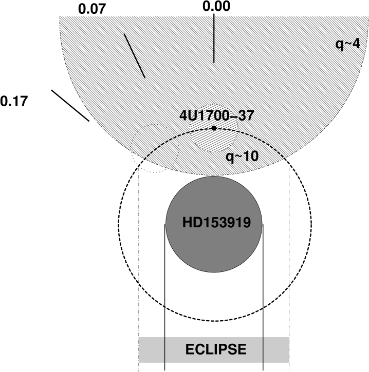
Figure 7: This sketch of the geometry of 4U 1700$-$37 includes the size of the region where q $\lesssim 4$, the upper limit on the size of the ionised region reported by van Loon et al. (2001)

If we compare the flux of the direct component in egress to that in low flux, we find that a similar decrease in the scattered component should result in a non-detection. A strong reduction of the flux of the direct component and consequently of the scattered component as inferred from model B can be explained by a reduction in accretion, such as the case in a “clumped” wind structure. Sako et al. (1999) also find evidence for clumping in the stellar wind of the optical companion of Vela~X$-$1. In case of Bondi-Hoyle accretion, often used to explain the production of X-rays in wind-accreting HMXBs (e.g Nagase 1989), the amount of material accreted (and thus L_X) scales as $\rho/v^{3}$, where $\rho$ is the density of the accreted material and $v$ its velocity. Therefore, the accretion is very sensitive to changes in the density- and (especially) in the velocity structure of the stellar wind (see Kaper et al. 1993). The X-ray lightcurve (see Fig. 1) shows strong variability, which suggests a continuously changing accretion rate onto the compact object. Given the duration of the low-flux interval ($\sim 5$ ks) and assuming a typical wind velocity $v\sim 1000$ km s^-1 the region should extend upto $\sim 5\times 10^{11}$ cm (i.e. $\sim 0.4\leavevmode\nobreak\ {\rm R}_{\star}$; Clark et al. 2002).

Model A can only be consistent with this scenario if the scattered component is not affected by the drop in accretion, since this model predicts a scattered component with a similar unabsorbed flux as the direct component. This is only possible if it is produced sufficiently far out in the system, that it does not notice a change in accretion rate for $\sim 5$ ks. This would require a distance of $\sim 10^{14}$ cm ($\sim 70{\rm R}_{\star}$), whereas the orbital separation of the compact object and the optical companion is $\sim 2\leavevmode\nobreak\ {\rm R}_{\star}$ (Heap & Corcoran 1992). This is not consistent with the relatively high column density (N${}_{\rm H}\sim 7\times 10^{22}$ cm^-2) toward the scattered component.

A possible alternative scenario that can be described by model A is the presence of an accretion wake, formed in front of the compact object, which creates a kind of eclipse that blockes the photons originating from the direct surroundings of the compact object. The presence of such a wake has been suggested by Haberl et al. (1994), based on a difference in the temperature of the bremsstrahlung component found in Ginga observations. In this scenario the interval of low flux should be locked to orbital phase, which is not consistent with other observations that report on low-flux intervals at different orbital phases. Boroson et al. (2003) find a quiescence period in Chandra observations around $\phi\sim 0.68$. Therefore, model A does not give a good physical description of the low-flux spectrum.

In the case of an exponential cutoff, the values of $E_{c}$ and $E_{f}$ can not be determined very well, due to the energy range of the EPIC/MOS-2 camera, but using fixed values for $E_{c}$ and $E_{f}$ in eclipse and egress, model B can be used to describe all three spectra. There is an indication for an increase of the photon index from eclipse and egress to the low-flux interval. Although the value of the photon index is correlated to the value of $E_{f}$, one can not exclude a change in the physical conditions of the accretion during the low-flux interval.

We conclude that model B probably best describes the physical conditions of the low-flux interval, in which the scattered component is not detected. A broader energy range is needed to further constrain the parameters of the high-energy cutoff.

4.2 Soft excess

A soft excess is clearly present in all spectra and can be modelled with components of different physical nature, modified by an absorption which is consistent with the interstellar value for this source. The previously reported bremsstrahlung component (Haberl & Day 1992; Haberl et al. 1994) results in a fit with a temperature that can not be constrained and a shape that mimics a power law. Also in the analysis of previously obtained data, the temperature of the bremsstrahlung component had to be fixed (e.g. Haberl et al. 1994; Reynolds et al. 1999). Therefore, we do not obtain more information on the physical origin of this component than with a simple power law model.

Another possible model for the soft excess is blackbody emission. This component is often visible in HMXBs hosting an accretion disc (e.g. LMC~X$-$4 and Cen~X$-$3; La Barbera et al. 2001 and Burderi et al. 2000, respectively). We can calculate the size of the emitting surface of the blackbody component:

$$R_{\rm km}=3.05\times 10^{9}d_{\rm kpc}F^{0.5}T_{\rm keV}^{-2}\leavevmode\nobreak\ ,$$ (2)

in which $R_{\rm km}$ is the radius of the emitting surface in km, $d_{\rm kpc}$ the distance to the source in kpc, $F$ the flux in erg s^-1 cm^-2 and $T_{\rm keV}$ the temperature in keV. Adopting a distance of 1.9 kpc (Ankay et al. 2001), we find an upper limit for the radius of the emitting volume of 52 km for the low-flux spectrum. For the eclipse and the egress spectrum we find upper limits for the radius of 0.13 and 0.34 km, respectively. These latter values are very small. Adding the fact that the absorption is very low, the blackbody component can not originate from an accretion disc or (close to) the compact object. We therefore conclude that although the soft excess can be described by a blackbody component, a proper physical interpretation is lacking.

The last possible continuum model which fits the soft excess is scattering. We examined both dust scattering and Thomson scattering. Dust scattering is energy dependent ($\propto 1/E^{2}$), which results in a steeper power law, mainly influencing the high-energy part of the spectrum. The difference between dust- and Thomson scattering can only be measured if the high energy part of the spectrum is not dominated by the strong direct component, i.e. during eclipse. Using dust scattering in eclipse does not improve the fit, whereas Thomson scattering does. Furthermore, this component has to originate from the outskirts of the system due to its low absorption. This is not consistent with a continuum that is absorbed in the extended stellar wind on its way out, before it is partly scattered. Therefore, we conclude that although Thomson scattering is a model that fits the data well in all cases, it is unlikely to be the physical origin of the soft excess.

Recently, Boroson et al. (2003) reported on Chandra observations of 4U~1700$-$37. They claim that the soft excess can be explained by a blend of lines only. However, the statistics of their observations are low at these energies and they only report one unresolved line below 1 keV. We tried to fit the soft excess in our spectra in a similar way by removing the soft continuum component and using broad gaussians to create a pseudo-continuum. Although this results in stable fits, the lines are 4–5 times broader than the energy resolution of EPIC/MOS-2 at low energies. Furthermore, the absorption of the direct and scattered component is $\sim 3$ times lower in eclipse than in egress. We conclude that this model does not provide a satisfying physical description of the continuum. However, it does not exclude the possible presence of a blend of lines. Therefore, it remains a matter of debate whether the soft excess is real or due to a blend of unresolved emission lines.

4.3 The Fe-line complex

The line spectrum consists of fluorescence emission lines of near-neutral species and discrete recombination lines of He- and H-like species. In eclipse and egress many lines are detected, while the low-flux spectrum shows only a few. Many lines are blended with each other or have multiple identifications, which complicates the analysis.

One of the most striking results is that the iron K$\alpha$ complex around 6.4 keV is strongly reduced in flux in the low-flux spectrum (see Fig. 5), while it is clearly visible in the rest of the (piled up) lightcurve. This is consistent with the reduced flux of the continuum above 6.4 keV and therefore another argument in favor of the scenario invoking a reduced accretion rate during the low-flux interval.

Moving from eclipse into egress, we find an increase by a factor $\sim 2$ of the flux of the Fe K$\alpha$ line at 6.4 keV. This suggests that the formation region of the fluorescence lines from near-neutral elements is not far from the compact object. However the presence of discrete recombination lines from He- and H-like elements indicates a highly ionised region. In some systems an accretion disc may be the source of these emission lines (e.g. LMC~X$-$4; La Barbera et al. 2001). However, 4U~1700$-$37 is a wind accreting system, for which no evidence for an accretion disc has been found. Another possible scenario (e.g. Sako et al. 2002) relates to the clumping of the stellar wind. If the wind is inhomogeneous, cool dense regions can form the near-neutral material, responsible for the presence of the fluorescence lines. This would result in a hybrid medium of cool dense and highly ionised regions.

The expected K$\beta$/K$\alpha$ ratio for an optically thin plasma (Kaastra & Mewe 1993) should be around 0.13. In Sect. 3.2.1 we show this is the case for eclipse, but in egress this is only true if the Fe edge is shifted to a slightly higher energy ($7.17_{-0.02}^{+0.01}$ keV). An edge at such energy can be produced by slightly more ionised iron, upto Fe iii (Lotz 1968). Ionisation stages of iron like Fe iii and Fe iv are abundant in the stellar winds of OB supergiants and are important wind drivers. Although we can exclude the edge to be produced by Fe iv or higher, this is not consistent with the results of Vink et al. (2000) who find that the stellar winds of OB-stars with temperatures higher than 25000 K are line driven by Fe iv, which recombines to Fe iii at larger distances from the stellar photosphere, typically around ${\rm R}\sim 6-8\leavevmode\nobreak\ {\rm R_{\star}}$ (Vink et al. 1999). This is beyond the orbital separation of $\sim 2\leavevmode\nobreak\ {\rm R}_{\star}$ (Heap & Corcoran 1992) and thus outside the region probed by the compact object during the egress interval (see Fig. 7).

4.4 Recombination lines

We detect discrete recombination lines in both the eclipse and the egress spectra. The emission lines reported in Sect. 3.2 can be identified with He- and H-like ions, with ionisation parameters in the range $2\lesssim{\rm log\leavevmode\nobreak\ }\xi\lesssim 4$. If we compare the flux of the lines that are clearly separated and have a unique identification, as a function of ${\rm log\leavevmode\nobreak\ }\xi$, we see a systematic change in flux of some of the lines from eclipse to egress. The elements with ${\rm log\leavevmode\nobreak\ }\xi\gtrsim 2.7$, i.e. ${S\textsc{xv}}\leavevmode\nobreak\ {\rm He\alpha}$, ${Ar\textsc{xvii}}\leavevmode\nobreak\ {\rm He\alpha}$ and ${Fe\textsc{xxv}}\leavevmode\nobreak\ {\rm He\alpha}$, grow in strength (see Fig. 6), while ${Si\textsc{xiv}}\leavevmode\nobreak\ {\rm Ly\alpha}$, ${Si\textsc{xiii}}\leavevmode\nobreak\ {\rm He\alpha}$ and ${Ne\textsc{x}}\leavevmode\nobreak\ {\rm Ly\alpha}$ remain constant within their errors. The observation of discrete recombination lines in an eclipse spectrum directly implies that the formation region extends beyond the size of the O supergiant. In our observations the eclipse interval covers a range in orbital phase of $0.07\leq\phi\leq 0.14$; therefore, the size of the ionised region should be $\sim 0.5\leavevmode\nobreak\ {\rm R}_{\star}$ (see Fig. 7). Because the lines with ${\rm log\leavevmode\nobreak\ }\xi\gtrsim 2.7$ are stronger in egress, the Strömgren zone, often defined as an ionised region with ${\rm log\leavevmode\nobreak\ }\xi\sim 3$, can not be too large.

At these relatively high values of $\xi$ inside this ionised region ions like C iv, Si iv and N v should be totally absent, resulting in an observable modulation of the UV resonance lines formed by these ions. This orbital modulation of UV resonance lines has been predicted for 4U~1700$-$37 by Hatchett & McCray (1977), but has never been observed (Dupree et al. 1978; Kaper et al. 1993). A possible explanation for the absence of the Hatchett-McCray (HM) effect in 4U~1700$-$37 is that the stellar wind has a non-monotonic (“turbulent”) velocity structure which can hide the presence of an ionisation zone from detection in an UV resonance line (Kaper et al. 1993).

van Loon et al. (2001) derive the size of the ionisation zone for a few HMXBs, based on a wind model taking the non-monotonic velocity structure into account. The size of the ionisation zone can also be expressed (Hatchett & McCray 1977) in terms of the non-dimensional variable $q$, that is defined as

$$q=\frac{\xi n_{\mathrm{X}}D^{2}}{L_{\mathrm{X}}},$$ (3)

where $\xi$ is the ionization parameter, $L_{\mathrm{X}}$ the X-ray luminosity, $n_{X}$ the number density at the orbit of the ionising source and $D$ the distance from the center of the O supergiant to the ionising source. Substitution of eq. 1 in eq. 3 then yields

$$q=\frac{n_{\mathrm{X}}D^{2}}{nr^{2}}.$$ (4)

In a medium with constant density, each value of $q$ corresponds to a circle centered on the X-ray source, where the radius increases with decreasing value of $q$. In a stellar wind, the density falls off roughly as $r_{\star}^{-2}$, such that surfaces of constant $q$ are small and closed (high $q$ value; see Fig. 7) or large and open with the ionising source off-center (low $q$; van Loon et al. 2001). To each value of $q$ corresponds a value of $\xi$, i.e. the higher the degree of ionisation, the higher the value of $q$. For 4U~1700$-$37 van Loon et al. (2001) set an upper limit of $q\sim 4$ to the size of the ionisation zone based on the absence of the HM effect in HD~153919 (see Fig. 7). They predict that $q$ must be of the order 200, for ${\rm log\leavevmode\nobreak\ }\xi=3$. Such a region would be much smaller than the size of the O supergiant. The detection of discrete recombination lines with high $\xi$ values during the eclipse spectrum indicates that the size of the ionisation zone must be larger, which is still consistent with the reported value for the upper limit, $q\lesssim 4$ (van Loon et al. 2001).

5 Summary and conclusions

XMM-Newton observations of 4U1700$-$37 during eclipse ($0.07\leq\phi\leq 0.14$) and egress ($0.14\leq\phi\leq 0.17$), as well as a low-flux interval around $\phi\sim 0.25$, produced the following results:

• The continuum is well represented by a combination of two power-law components: (i) a direct component produced by the X-ray source and (ii) a (Thomson) scattered component originating in an extended region surrounding the X-ray source. The extent of this region must exceed the size of the O supergiant as the scattered component is detected during eclipse.

• The low-flux interval is likely due to a lack of accretion onto the compact object due to a varying density and/or velocity structure of the accreting material, such as expected for a clumpy stellar wind of the optical companion.

• At low energies ($\lesssim 2$ keV) a soft excess is present, similar to what has been found in earlier observations with, e.g. EXOSAT and Ginga. We can exclude a thermal origin in the form of bremsstrahlung or blackbody emission.

• In all spectra we detect fluorescence line emission from near-neutral iron around 6.4 keV, probably produced by dense “clumps” in the stellar wind close to the compact object. In the low-flux interval this line is strongly reduced in flux in tandem with the continuum above 6.4 keV.

• The initially measured high Fe K$\beta$/K$\alpha$ ratio in egress can be explained by an Fe edge due to moderately ionised iron, upto Fe iii. This is consistent with the ionisation degree of iron further out in the stellar wind of the optical companion, but not with the region probed by the compact object in egress.

• We detect many discrete recombination lines from He- and H-like species in both eclipse and egress. Some of the lines can be isolated, while most of them are blended with each other. The presence of these lines in eclipse directly implies that the formation region has a minimum size of around $0.5{\rm R}_{\star}$. Some of the lines with a relatively high value of the ionisation parameter $\xi$ grow stronger towards egress. This implies that the ionisation zone can not be very large either.