Gamma-Ray Bursts: Polarization of Afterglows from Two-Component Jets

Abstract

Polarization behaviors of optical afterglows from two-component gamma-ray burst jets are investigated, assuming various configurations for the two components. In most cases, the observed polarization is dominated by the inner narrow component for a long period. Interestingly, it is revealed that different assumptions about the lateral expansion of the jet can lead to different evolutions of the position angle of polarization. The observed afterglow light curve and polarization behaviors of GRB $020813$ can be well explained by the two-component jet model. Particularly, the model is able to explain the constancy of the observed position angle in this event, given that the line of sight is slightly outside the narrow component.

1 Introduction

Soon after the discovery of gamma-ray burst (GRB) afterglows, it was expected that radiation from these GRB embers may be polarized (Loeb & Perna 1998; Gruzinov & Waxman 1999; Medvedev & Loeb 1999). The first direct detection of polarized afterglows from GRB $990510$ by Covino et al. (1999) and later confirmation by Wijers et al. (1999) intrigued subsequent investigations of the geometry of GRB ejecta (Ghisellini & Lazzati 1999; Sari 1999; Gruzinov 1999).

Polarization originates naturally from some asymmetries when relativistic electrons produce non-thermal radiation. To model the observed polarizations of GRB afterglows, there are basically two kinds of consideration on the violation of symmetry with respect to the observer. The first class includes the models assuming ordered magnetic fields. The magnetic fields can be either locally ordered, which corresponds to the magnetic domain model (Gruzinov & Waxman 1999), or even entirely aligned within the ejecta which is magnetized by the central engine (Granot & Königl 2003; Lyutikov, Pariev & Blandford 2003; Lazzati et al. 2004; Dai 2004). The second class involves beaming effect, where the GRB ejecta is assumed to be conically collimated. Observers need to be off-axis, which is natural since a large viewing angle corresponds to a large chance possibility. The magnetic fields are postulated to be randomly but an-isotropically distributed behind the shock. The simplest configuration is two dimensional, with the magnetic fields randomly distributed in the shock plane (Ghisellini & Lazzati 1999; Laing 1980). In further particular advisements the level of the magnetic field anisotropy has been parameterized (Gruzinov 1999; Sari 1999; Granot & Königl 2003). Previous works revealed that the simple homogeneous jet is confronted with abrupt variation of polarization angle by $90^{\circ}$, when the degree of polarization passes through zero. No intermediate values for the position angle are expected in this model. In fact, the observed position angle of some afterglows, e.g. GRBs $990712$ (Rol et al. 2000), $020405$ (Covino et al. 2003a) and $020813$ (Gorosabel et al. 2004), did not exhibit such significant changes. As indicated by simulations of jet propagating in the collapsar, the emergent jet from the stellar envelope is structured (Zhang, Wooley & Heger 2004). Two approximations on the jet structure had been made previously. One is the power law structure (Mészáros, Rees & Wijers 1998; Dai & Gou 2001; Rossi, Lazzati & Rees 2002), while the other is the Gaussian profile (Zhang & Mészáros2002). Recently, Rossi et al. (2004) had detailedly investigated the polarization behavior of both a power law structured jet and a Gaussian jet. The advantage of these kinds of structured jets is that the position angle keeps constant with time.

In this paper we explore the polarization of GRB afterglows by assuming a different jet structure, i.e. the two-component jet structure. The two-component jet model was proposed to explain observations, such as unusual radio to X-ray spectrum and late time bumps in some afterglows (Frail et al. 2000; Berger et al. 2003; Huang et al. 2004). Liang & Dai (2004) found that there exist two peaks in the histogram of the spectral peak energy distribution derived from $\nu F_{\nu}$ in GRBs, which also tentatively implies a two-component structure of GRB jets. In Section 2 we describe the dynamics and radiation mechanism of two-component jets. The afterglow polarization behavior of two-component jets is presented in Section 3. Observed light curve and polarization curve of GRB $020813$ are fitted within this model in Section 3.3. We conclude and discuss our results in Section 4. In the Appendix, the polarization degree of synchrotron radiation in an ordered magnetic field as a function of frequency is given.

2 Jet hydrodynamics and synchrotron radiation

For simplicity, we make several assumptions on the hydrodynamic evolution of a two-component jet. First, the two-component jet evolves adiabatically. Second, we apply the uniform thin shell approximation to both components of the jet. Third, we assume that there is no interaction between the narrow and wide components. Each component evolves independently and therefore can be treated separately (see also Huang et al. 2004). Lastly, two different assumptions are made on the lateral expansion of the jet. One is to assume that the jet expands laterally at the speed of light, and the other is to postulate that the jet experiences no lateral expansion. The former corresponds to the case of a clear-cut lateral boundary between the uniform jet and the environment, which was assumed for simplicity in previous works (Rhoads 1999; Sari, Piran, $\&$ Halpern 1999). However, the physical parameters near the actual lateral boundary should vary gradually (Zhang et al. 2004). Recent hydrodynamical calculations showed that for smooth jet profiles the lateral expansion speed is much less than the sound speed in the jet co-moving frame even during the relativistic stage (Kumar $\&$ Granot 2003; Granot $\&$ Kumar 2003). So, whether the jet expands laterally or not is still an open question. We therefore also discuss the second possibility that the jet has no sideways expansion. In the following, we denote the physical parameters of the narrow and wide components by the subscripts “N” and “W”, respectively. The narrow (wide) component can be described by the isotropic kinetic energy $E_{N,iso}$ ($E_{W,iso}$), the bulk Lorentz factor $\gamma_{N}$ ($\gamma_{W}$), and the half-opening angle $\theta_{N}$ ($\theta_{W}$).

The hydrodynamic evolution can be evaluated in the same way for both components of the jet. One caveat should be made about the inner boundary of the wide component. The wide component is assumed to be a hollow cone, with the inner half-opening angle to be constant and the same as the initial aperture of the narrow component during the whole relativistic stage. However, the hydrodynamics of the wide component should be hardly affected by this fact. We let $\theta_{0}$ be the initial half-opening angle of an arbitrary component. After a short coasting phase or reverse-forward shock interaction epoch, the jet begins to decelerate in the interstellar medium (ISM), with its radius $R$, bulk Lorentz factor $\gamma$ and half-opening angle $\theta_{j}$ evolve as (Sari, Piran, $\&$ Narayan 1998)

$$R=5.8\times 10^{17}E_{53}^{1/4}n^{-1/4}t_{d}^{1/4}(\frac{1+z}{2})^{-1/4}\,\,\rm{cm,}$$ (1)

$$\gamma=11E_{53}^{1/8}n^{-1/8}t_{d}^{-3/8}(\frac{1+z}{2})^{3/8},\phantom{ssss}\theta_{j}\approx\theta_{0},$$ (2)

where the isotropic kinetic energy $E=10^{53}E_{53}$ erg, the ISM number density $n$ is in units of cm^-3, $t_{d}$ is the observer’s time in days, and $z$ is the redshift. During this stage, the hydrodynamics of the jet is the same as that of an isotropic fireball, which obeys the self-similar solution of Blandford-McKee (1976). As the jet continues to decelerate, there is a critical moment when the Lorentz factor $\gamma=\theta_{0}^{-1}$, which corresponds to the time

$$t_{j}=0.645(1+z)E_{53}^{1/3}n^{-1/3}\theta_{0,-1}^{8/3}\,\rm{day},$$ (3)

where $\theta_{0}=0.1\theta_{0,-1}$. In the case of no lateral expansion, the jet hydrodynamics after this time is unchanged and still can be described by equations (1) and (2). On the other hand, if the jet expands laterally at the speed of light, the jet will experience a runway sideways expansion (Rhoads 1999; Sari et al. 1999). The hydrodynamic quantities in this case when $t>t_{j}$ evolve as

$$R=6.18\times 10^{17}E_{53}^{1/3}n^{-1/3}\theta_{0,-1}^{2/3}\,\rm{cm,}$$ (4)

$$\gamma=\theta_{0}^{-1}(\frac{t}{t_{j}})^{-1/2},\phantom{ssssssss}\theta_{j}\approx\gamma^{-1}.$$ (5)

Polarized afterglows have been observed usually within several days (Covino et al. 2002; Björnsson 2002). In this paper, we focus on the stage when the jet is still relativistic. The moment when the jet becomes non-relativistic is typically much later, unless the ISM density is very large and comparable to that of giant molecular clouds in the Galaxy (Dai & Lu 1999).

The post-shock electrons and magnetic fields are usually assumed to share the fractions $\epsilon_{e}$ and $\epsilon_{B}$ of the total internal energy, respectively. Therefore, the magnetic field in the co-moving frame is

$$B^{\prime}=\sqrt{32\pi\epsilon_{B}m_{p}n}\gamma c\approx 0.4\gamma\epsilon_{B}^{1/2}n^{1/2}\,\,\rm{G},$$ (6)

while the minimum Lorentz factor of accelerated electrons is (Huang et al. 2000)

$$\gamma_{m}=\epsilon_{e}\frac{p-2}{p-1}\frac{m_{p}}{m_{e}}(\gamma-1)+1,$$ (7)

where $m_{p}$ and $m_{e}$ are the proton and electron masses, and $p$ is the index of shock-accelerated electron distribution. The electrons can be cooled down within the dynamical time scale. The cooling Lorentz factor of electrons by purely synchrotron cooling is (Sari et al. 1998)

$$\gamma_{c}^{syn}=\frac{6\pi m_{e}c(1+z)}{\sigma_{\rm{T}}\gamma B^{\prime 2}t},$$ (8)

where $c$ is the speed of light and $\sigma_{\rm{T}}$ is the Thomson cross section. Further cooling of electrons by inverse-Compton (IC) up-scattering of the primary synchrotron photons can reduce the above cooling Lorentz factor (Waxman 1997; Wei & Lu 1998; Panaitescu & Kumar 2000). Following Sari & Esin (2001), we get the final cooling Lorentz factor

$$\gamma_{c}=\frac{\sqrt{1+4\displaystyle\frac{\epsilon_{e}}{\epsilon_{B}}}-1}{2\displaystyle\frac{\epsilon_{e}}{\epsilon_{B}}}\gamma_{c}^{syn}\approx\left\{\begin{array}[]{l}\gamma_{c}^{syn},\phantom{ssssss}\epsilon_{e}\ll\epsilon_{B},\\ \sqrt{\displaystyle\frac{\epsilon_{B}}{\epsilon_{e}}}\gamma_{c}^{syn},\phantom{s}\epsilon_{e}\gg\epsilon_{B},\\ \end{array}\right.$$ (9)

in the fast-cooling phase ($\gamma_{c}<\gamma_{m}$), and

$$\gamma_{c}\approx\left\{\begin{array}[]{l}\displaystyle(\sqrt{\frac{\epsilon_{B}}{\epsilon_{e}}}\frac{\gamma_{c}^{syn}}{\gamma_{m}})^{2/(4-p)}\gamma_{m},\phantom{s}\gamma_{c}^{syn}\leq(\frac{\epsilon_{e}}{\epsilon_{B}})^{1/(p-2)}\gamma_{m},\\ \displaystyle\gamma_{c}^{syn},\phantom{ssssssssssssssssss}\gamma_{c}^{syn}\geq(\frac{\epsilon_{e}}{\epsilon_{B}})^{1/(p-2)}\gamma_{m},\\ \end{array}\right.$$ (10)

in the slow-cooling phase ($\gamma_{m}<\gamma_{c}$). In deriving the above $\gamma_{c}$ we adopt $2<p<4$, which seems to be easily satisfied by both the theoretical prediction and observations (Wu, Dai, & Liang 2004). It can be seen from equations (9) and (10) that $\gamma_{c}$ always equals to $\gamma_{c}^{syn}$ for $\epsilon_{e}\leq\epsilon_{B}$. In the case of $\epsilon_{e}>\epsilon_{B}$, the evaluation of $\gamma_{c}$ is considered in three evolutionary stages. Equation (9) describes the first IC-dominated fast-cooling case, while equation (10) represents the following IC-dominated and then synchrotron-dominated slow-cooling cases. The two characteristic frequencies of synchrotron radiation in the co-moving frame are the typical frequency $\nu_{m}^{\prime}=\displaystyle\frac{eB^{\prime}}{2\pi m_{e}c}\gamma_{m}^{2}$ and the cooling frequency $\nu_{c}^{\prime}=\displaystyle\frac{eB^{\prime}}{2\pi m_{e}c}\gamma_{c}^{2}$, which corresponds to the electrons with minimum Lorentz factor $\gamma_{m}$ and with cooling Lorentz factor $\gamma_{c}$, respectively. Sari et al. (1998) showed that the co-moving peak spectral power per electron is independent of the electron energy, i.e. $P^{\prime}_{\nu^{\prime},max}=\displaystyle\frac{m_{e}c^{2}\sigma_{\rm{T}}}{3e}B^{\prime}$, where $e$ is the electron charge. The co-moving peak intensity is therefore (Rossi et al. 2004)

$$I^{\prime}_{\nu^{\prime},max}=\frac{P^{\prime}_{\nu^{\prime},max}}{4\pi}\frac{nR}{3}=\frac{m_{e}c^{2}\sigma_{\rm{T}}}{36\pi e}B^{\prime}nR.$$ (11)

The spectral energy distribution of synchrotron radiation can be constructed by the characteristic frequencies $\nu_{c}^{\prime}$, $\nu_{m}^{\prime}$ and the peak intensity $I^{\prime}_{\nu^{\prime},max}$. In the fast-cooling phase ($\nu_{c}^{\prime}<\nu_{m}^{\prime}$), we have

$$I^{\prime}_{\nu^{\prime}}=I^{\prime}_{\nu^{\prime},max}\times\left\{\begin{array}[]{l}\displaystyle(\frac{\nu^{\prime}}{\nu^{\prime}_{c}})^{1/3},\phantom{sssssssssssss}\nu^{\prime}<\nu^{\prime}_{c},\\ \displaystyle(\frac{\nu^{\prime}}{\nu^{\prime}_{c}})^{-1/2},\phantom{sssssssssss}\,\nu^{\prime}_{c}<\nu^{\prime}<\nu^{\prime}_{m},\\ \displaystyle(\frac{\nu^{\prime}_{m}}{\nu^{\prime}_{c}})^{-1/2}(\frac{\nu^{\prime}}{\nu^{\prime}_{m}})^{-p/2},\phantom{s}\,\nu^{\prime}_{m}<\nu^{\prime},\\ \end{array}\right.$$ (12)

and in the slow-cooling phase ($\nu_{m}^{\prime}<\nu_{c}^{\prime}$), we have

$$I^{\prime}_{\nu^{\prime}}=I^{\prime}_{\nu^{\prime},max}\times\left\{\begin{array}[]{l}\displaystyle(\frac{\nu^{\prime}}{\nu^{\prime}_{m}})^{1/3},\phantom{sssssssssssss}\nu^{\prime}<\nu^{\prime}_{m},\\ \displaystyle(\frac{\nu^{\prime}}{\nu^{\prime}_{m}})^{-(p-1)/2},\phantom{ssssssss}\nu^{\prime}_{m}<\nu^{\prime}<\nu^{\prime}_{c},\\ \displaystyle(\frac{\nu^{\prime}_{c}}{\nu^{\prime}_{m}})^{-(p-1)/2}(\frac{\nu^{\prime}}{\nu^{\prime}_{c}})^{-p/2},\nu^{\prime}_{c}<\nu^{\prime}.\\ \end{array}\right.$$ (13)

We do not include the synchrotron-self-absorption effect which may be important mainly at the radio wavelength. Since afterglow polarizations had been detected mostly in optical bands, we will only investigate the temporal evolution of optical polarization.

3 Polarization

3.1 Formulation

Figure 1: Projection of a two-component jet. The inner cone is the narrow component, and the outer hollow cone is the wide component. The viewing angle between the jet axis (C.A.) and the line of sight (LOS) is $\theta_{V}$. Also shown are the apertures relative to the origin of the GRB jet, with $\theta_{N}$ of the narrow component and $\theta_{W}$ of the wide component. An arc centered to LOS with aperture $\theta$ (dotted line) is divided into three segments, with the segment ($\chi_{N}$,$2\pi-\chi_{N}$) in the narrow component and the segments ($\chi_{W}$,$\chi_{N}$) and ($2\pi-\chi_{N}$,$2\pi-\chi_{W}$) in the wide component.

The polarization of emission from a point-like region averaged by the distribution of the post-shock tangled magnetic field is (Sari 1999; Gruzinov 1999)

$$\Pi(\gamma,\theta)=\Pi_{0}\delta^{2}(\gamma,\theta)\sin^{2}\theta\frac{{\xi^{2}-1}}{{2\xi^{2}+(1-\xi^{2})\delta^{2}(\gamma,\theta)\sin^{2}\theta}},$$ (14)

where $\theta$ is the angle between the velocity vector of the emitting point and the line of sight, $\delta(\gamma,\theta)=\displaystyle\frac{1}{\gamma(1-\beta\cos\theta)}$ is the Doppler boosting factor. The parameter $\xi^{2}=\langle B_{\perp}^{2}\rangle/2\langle B_{\parallel}^{2}\rangle$ denotes the level of anisotropy of the magnetic field distribution, where $B_{\perp}$ and $B_{\parallel}$ are magnetic field components perpendicular and parallel to the normal of the shock plane. The triangular brackets mean that the quantity inside is averaged over the solid angles. $\Pi_{0}$ is the linear polarization degree of synchrotron photons emitted by the electrons in an ordered magnetic field. For an isotropic power-law distribution of electrons with index $p$, the approximate $\Pi_{0}=(p+1)/(p+7/3)$ holds true for a wide range of frequencies. The exact dependence of $\Pi_{0}$ on the frequency is given in the Appendix (see Figure A1). Using the above approximate expression for $\Pi_{0}$ actually leads to neglectable errors in the final results. We therefore adopt the usual approximate value of $\Pi_{0}$ in the following calculations.

To determine the total polarization of a GRB jet, we need to integrate the Stokes parameters over the jet surface. From Figure 1, by virtue of spherical geometry we have

$$\chi_{i}(\theta)=\left\{{\begin{array}[]{c}\phantom{sssss}\pi\Theta(\theta_{V}-\theta_{j})\phantom{ssssssss},{\theta<\theta_{-}},\\ {\pi-\cos^{-1}(\displaystyle\frac{{\cos\theta_{j}-\cos\theta\cos\theta_{V}}}{{\sin\theta\sin\theta_{V}}})},\phantom{}{\theta_{-}<\theta<\theta_{+}},\\ \phantom{ssssssssss}\pi\phantom{sssssssssssss},{\theta_{+}<\theta},\\ \end{array}}\right.$$ (15)

where $\theta_{V}$ is the observer’s viewing angle with respect to the jet axis, $\theta_{-}=\mid\theta_{j}-\theta_{V}\mid$, and $\theta_{+}=\theta_{j}+\theta_{V}$. $\Theta(x)$ is the heaviside step function with $\Theta(x>0)=1$ and $\Theta(x<0)=0$. Note that equation (15) is valid for both components, i.e. $\chi_{i}=\chi_{N}$ when $\theta_{j}=\theta_{N}$, and $\chi_{i}=\chi_{W}$ when $\theta_{j}=\theta_{W}$. Ghisellini & Lazzati (1999) have given an approximate expression of $\chi_{i}$ ($\psi_{1}$ in their work) for the intermediate case. Integrating over each component of the jet, we get the Stokes parameters as

$${Q}_{i}(t,\nu)=\frac{{1+z}}{{D_{\rm{L}}^{2}}} \int_{0}^{\theta_{V}+\theta_{W}}{\delta^{3}(\gamma_{i},\theta)I^{\prime}_{\nu^{\prime},i}}\Pi(\gamma_{i},\theta)R_{i}^{2}\sin\theta d\theta$$ (16)

$$\times\int_{\chi_{i,min}}^{\chi_{i,max}}{\cos 2\varphi d\varphi},$$

$${I}_{i}(t,\nu)=\frac{{1+z}}{{D_{\rm{L}}^{2}}} \int_{0}^{\theta_{V}+\theta_{W}}{\delta^{3}(\gamma_{i},\theta)I^{\prime}_{\nu^{\prime},i}}R_{i}^{2}\sin\theta d\theta$$ (17)

$$\times\int_{\chi_{i,min}}^{\chi_{i,max}}{d\varphi},$$

where $i=W$ or $N$, $\nu^{\prime}=(1+z)\delta^{-1}(\gamma_{i},\theta)\nu$ is the frequency in the co-moving frame. For the narrow component, $\chi_{N,min}=\chi_{N}(\theta)$ and $\chi_{N,max}=2\pi-\chi_{N}(\theta)$. For the wide component, the azimuthal integral is from $\chi_{W,min}=\chi_{W}(\theta)$ to $\chi_{W,max}=\chi_{N,0}(\theta)$, and again from $\chi_{W,min}=2\pi-\chi_{N,0}(\theta)$ to $\chi_{W,max}=2\pi-\chi_{W}(\theta)$. Here $\chi_{N,0}(\theta)$ is calculated by inserting the inner half-opening angle of the wide hollow cone $\theta_{N,0}$ into equation (15), where $\theta_{N,0}$ is the initial aperture of the narrow component. Note that Stokes parameter $U_{N}=U_{W}=0$ can be easily derived from the symmetry. The Stokes parameters for the whole jet are therefore calculated by summation of the values of these two components,

$${Q}_{tot}(t,\nu)= \frac{{1+z}}{{D_{\rm{L}}^{2}}}\int_{0}^{\theta_{V}+\theta_{W}}\sin\theta d\theta\times$$

$$\{ {\delta^{3}(\gamma_{W},\theta)I^{\prime}_{\nu^{\prime},W}}\Pi(\gamma_{W},\theta)R_{W}^{2}(\sin 2\chi_{N,0}-\sin 2\chi_{W})$$ (18)

$$-\delta^{3}(\gamma_{N},\theta)I^{\prime}_{\nu^{\prime},N}\Pi(\gamma_{N},\theta)R_{N}^{2}\sin 2\chi_{N}\},$$

$${Q}_{tot}(t,\nu)= \frac{{1+z}}{{D_{\rm{L}}^{2}}}\int_{0}^{\theta_{V}+\theta_{W}}\sin\theta d\theta\times$$

$$\{ {\delta^{3}(\gamma_{W},\theta)I^{\prime}_{\nu^{\prime},W}}\Pi(\gamma_{W},\theta)R_{W}^{2}(\sin 2\chi_{N,0}-\sin 2\chi_{W})$$ (19)

$$-\delta^{3}(\gamma_{N},\theta)I^{\prime}_{\nu^{\prime},N}\Pi(\gamma_{N},\theta)R_{N}^{2}\sin 2\chi_{N}\},$$

$${I}_{tot}(t,\nu)= \frac{{1+z}}{{D_{\rm{L}}^{2}}}\int_{0}^{\theta_{V}+\theta_{W}}\{{\delta^{3}(\gamma_{W},\theta)I^{\prime}_{\nu^{\prime},W}}R_{W}^{2}(2\chi_{N,0}-2\chi_{W})$$ (20)

$$+\delta^{3}(\gamma_{N},\theta)I^{\prime}_{\nu^{\prime},N}R_{N}^{2}(2\pi-2\chi_{N})\}\sin\theta d\theta.$$

The total polarization of the two component jet is thus given by

$$P_{tot}=\displaystyle\frac{Q_{tot}}{I_{tot}}.$$ (21)

The corresponding polarization vector is either (anti-) parallel or perpendicular to the vector from C.A. to LOS projected in the sky (see Figure 1), depending on whether the magnetic field parameter $\xi^{2}$ is larger than unity or not, as well as on which direction the observer views and how the jet evolves (Ghisellini & Lazzati 1999; Sari 1999).

3.2 Numerical Results

Below we use several sets of physical parameters to illustrate the temporal evolution of afterglow polarization of a two-component jet. The main interesting parameter effects may arise from the ratio of the isotropic-equivalent energy of the two components $E_{W,iso}/E_{N,iso}$, and the ratio of their initial half-opening angles $\theta_{W,0}/\theta_{N,0}$. We fix other parameters and assume $E_{N,iso}=10^{53}$ erg, $\theta_{N,0}=0.05$, $n=1$ cm^-3, $\epsilon_{e}=0.1$, $\epsilon_{B}=0.01$, $p=2.2$, $\xi^{2}=9$ and $\Pi_{0}=60\%$ in the following calculations. The equal arrival time surface effect is neglected in this primary research. The adopted parameters of the cosmology are $\Omega_{m}=0.27$, $\Omega_{\Lambda}=0.73$, $H_{0}=71$ km s^-1 Mpc^-1, and the GRB is assumed to be located at $z=1.0$.

Figure 2 shows the light curves and polarization evolutions of GRB optical afterglows ($\nu_{opt}=4.5\times 10^{14}$ Hz) from two-component jets, which are assumed to evolve with no lateral expansions. The ratio of the wide component aperture to that of the narrow component is chosen to be $\theta_{W,0}/\theta_{N,0}=6$. The upper panel corresponds to a relatively low isotropic energy ratio as $E_{W,iso}/E_{N,iso}=0.1$, while the lower panel corresponds to a high ratio as $E_{W,iso}/E_{N,iso}=0.3$. When the line of sight is in the narrow component, i.e. $\theta_{V}<\theta_{N,0}$, the light curve differs little between each other since the light mainly comes from the narrow component. The light curve steepens from $\sim t^{-0.9}$ to $t^{-1.6}$ at around $t_{j,N}\sim 0.2$ day, which is shallow as expected for the non-lateral expansion jet (Mészáros & Rees 1999). The polarization degree is also dominated by the narrow component, and changes from an initially negative value to a later positive value, which means that the position angle of polarization changes by $90^{\circ}$. After reaching a maximum, the polarization decreases and approaches zero. When the line of sight lies within the wide component, the light curve flattens when the narrow component decelerates and enters into the field of view. The degree of flattening is determined by the viewing angle $\theta_{V}$ and the energy ratio $E_{W,iso}/E_{N,iso}$. The smaller $\theta_{V}$ or $E_{W,iso}/E_{N,iso}$ is, the more contribution is resulted from the narrow component, as can be seen in the figure. Contrary to the light curve, the total polarization follows almost the evolution of polarization of the narrow component for a long time. This is because the narrow component is off-viewed and the increase of the point polarization is greater than the decrease of the Doppler boosting when $\theta$ increases (equations 14 and 16). The only exception is when $\theta_{V}/\theta_{N,0}=5$, in which case the polarization evolution is dominated by the wide component. For the other cases, the polarization level is depleted to a certain extent by the wide component. In the cases of $\theta_{V}/\theta_{N,0}=1.2$ and $1.5$, there exist long periods with nearly constant polarization levels and unchanged position angles, which is the typical characteristics of off-viewed jets (Granot et al. 2002; Rossi et al. 2004). In general, increasing the contrast between $E_{W,iso}$ and $E_{N,iso}$ would decrease the maximum of polarization degree and reduce the flattening or bump by the central narrow component.

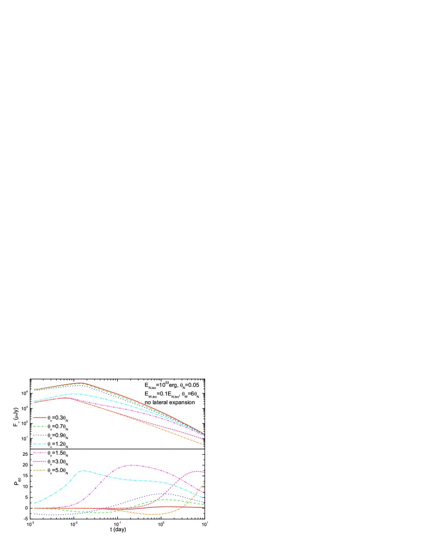
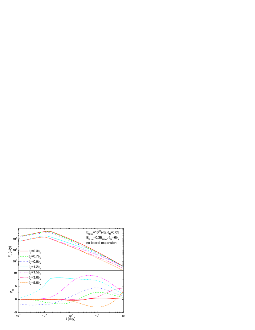
Figure 2: Light curves and polarization evolutions of GRB optical afterglows from two-component jets. The jet is assumed to have no lateral expansion. The contrasts between the wide and narrow component parameters are $E_{W,iso}/E_{N,iso}=0.1$ (upper panel) or $0.3$ (lower panel), and $\theta_{W,0}/\theta_{N,0}=6$. Different lines correspond to different viewing angles ($\theta_{V}$).

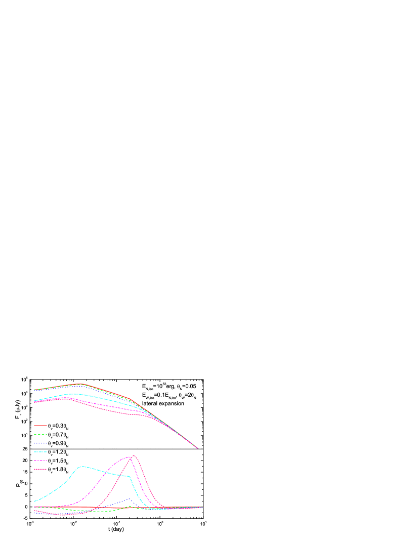
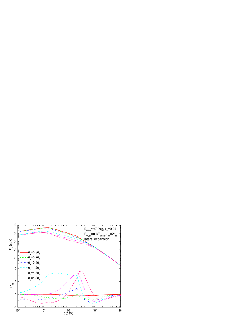
Figure 3: Light curves and polarization evolutions of GRB optical afterglows from two-component jets. The jet is assumed to expand laterally at the speed of light. The contrasts between the wide and narrow component parameters are $E_{W,iso}/E_{N,iso}=0.1$ (upper panel) or $0.3$ (lower panel), and $\theta_{W,0}/\theta_{N,0}=2$. Different lines correspond to different viewing angles ($\theta_{V}$).

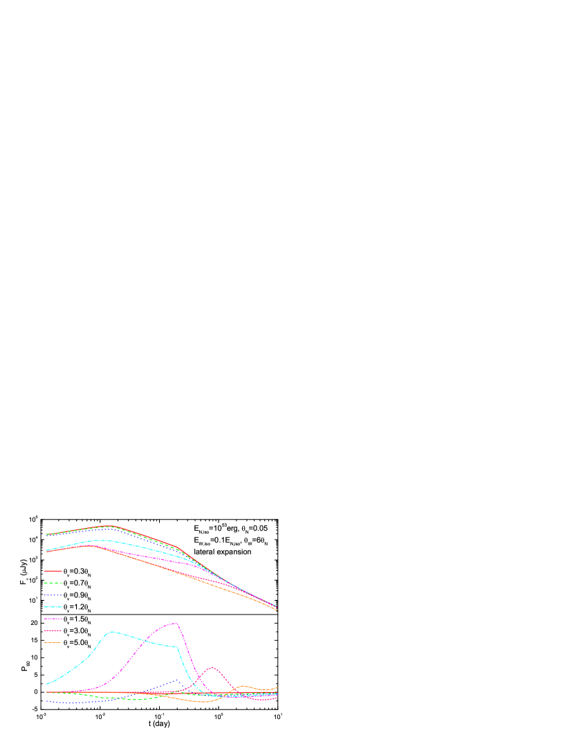
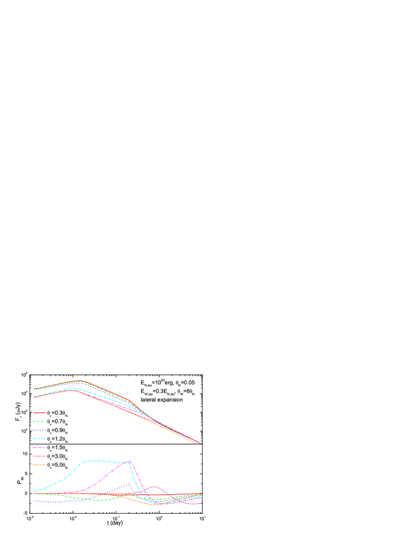
Figure 4: Same as Figure 3 except for $\theta_{W,0}/\theta_{N,0}=6$ now.

Figures 3 and 4 depict the light curves and polarization evolutions of GRB optical afterglows from two-component jets with lateral expansions. When $\theta_{V}<\theta_{N,0}$, the light curve is dominated by the narrow component and experience a steepening from $t^{-0.9}$ to $t^{-2.2}$ at $t_{j,N}\approx 0.2$ day. The light curve flattens at late times when the wide component begins to dominate over the narrow one for $\theta_{W,0}/\theta_{N,0}=6$, in which case the jet break of the wide component occurs at rather late times, $t_{j,W}>10$ days. The sign of polarization changes twice for $\theta_{V}<\theta_{N,0}$. In most cases, except when $\theta_{V}$ is very close to $\theta_{W,0}$, the polarization curves have one peak at around $t_{j,N}$. These are typical for jets with lateral expansion (Sari 1999). For $\theta_{V}>\theta_{N,0}$, the polarization is mainly dominated by the narrow component before $t_{j,N}$. Exceptions are $\theta_{V}=1.8\theta_{N,0}$ in the case of $\theta_{W,0}=2\theta_{N,0}$ and $\theta_{V}=5\theta_{N,0}$ in the case of $\theta_{W,0}=6\theta_{N,0}$, where the polarization is dominated by the wide component during the whole evolution. After the jet break the asymmetry of the narrow component diminishes due to sideways expansion, the polarization begins to be determined by the wide component, almost regardless of whether $\theta_{V}$ is larger than $\theta_{N,0}$ or not. In the figures we can see that the absolute polarization level at $t>t_{j,N}$ increases with $E_{W,iso}/E_{N,iso}$. As shown in the figures, the light curves in cases of $\theta_{V}>\theta_{N,0}$ are influenced by the narrow component through a bump or flattening. When the ratio $\theta_{W,0}/\theta_{N,0}$ or especially $E_{W,iso}/E_{N,iso}$ increases, the influence of the narrow component to the light curve is reduced, and the maximum polarization level also decreases.

There are mainly two differences between the scenario without lateral expansion and that with lateral expansion. The first is the temporal behavior of light curve after the jet break time $t_{j}$. The light-curve steepening of a non-lateral expansion jet around $t_{j}$ is relatively shallow, while the steepening of a lateral expansion jet is large. The second is the width of the peak in the temporal polarization curve. A jet with lateral expansion has a more narrow polarization peak than a jet without lateral expansion, as can be seen by comparing Figure 2 with Figure 3. Rossi et al. (2004) have investigated the polarization evolutions of structured jets, with both the power-law and Gaussian distributions. They found that the position angle of polarization is not changed in time for these structured jets. A two-component without lateral expansion also has an unchanged position angle when $\theta_{N,0}<\theta_{V}<\theta_{W,0}$ . The similarities between such two-component jets and those with power law or Gaussian structure are that they all have no or little lateral expansions and they are more energetic near the jet axis.

3.3 The case of GRB $020813$

The bright long duration GRB $020813$ detected by HETE-II spacecraft had been well-observed for evolutions of both optical flux density and polarization. The redshift of this burst is $z=1.255$, by identifying the [O II] $\lambda 3727$ line of the host galaxy (Barth et al. 2003). The light curve of GRB $020813$ afterglow is the smoothest one among GRBs localized so far (Laursen & Stanek 2003). The optical afterglow has a jet break around $0.33$ - $0.88$ day since the main burst (Gorosabel et al. 2004; see also Covino et al. 2003b, Li et al. 2003). The temporal index before the break ($\alpha_{1}$) is $\sim-0.55$ — $\sim-0.78$, and the index after the break ($\alpha_{2}$) is $\sim-1.44$ — $-1.75$. Barth et al. (2003) have obtained the afterglow spectrum in optical band, and found that the spectral index is $\beta=1.06\pm 0.01$. Assuming that the spectrum is fast cooling, the inferred power law index of electron distribution is $p=2.12\pm 0.02$. The spectropolarimetric observations had been made by Keck between $0.19-0.33$ days and by VLT between $0.88-4.05$ days (Barth et al. 2003; Gorosabel et al. 2004). The degree of polarization decreases from about $3\%$ to less than $1\%$, while the position angle varies slowly and can be regarded as constant. Both observations showed that the majority of these detected polarizations are intrinsic and not effected by the line-of-sight dust. Therefore, the afterglow of GRB $020813$ provides us an ideal sample to investigate the structure of GRB jets (Lazzati et al. 2004).

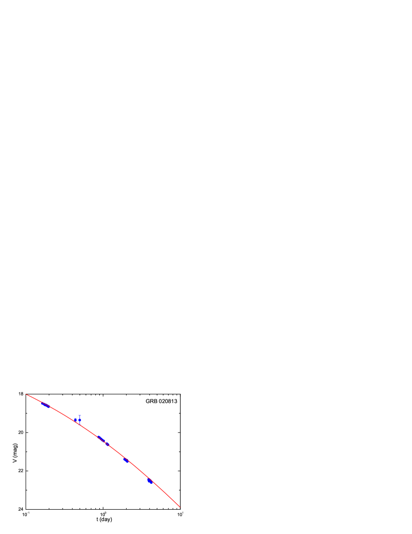
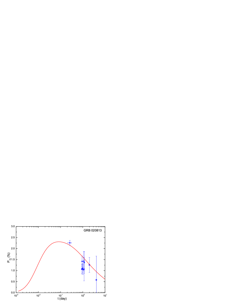
Figure 5: Fitting to the GRB 020813 V-band afterglow light curve (upper panel) and its polarization evolution (lower panel). The Galactic extinction in the V-band $A_{V}=0.42$ is adopted (Covino et al. 2003b).

We have fitted the V-band light curve and polarization evolution of GRB $020813$ afterglow in the context of the two-component jet model. The data of light curve and polarizations are taken from Gorosabel et al. (2004), in which they included and averaged the polarization observations made by Barth et al. (2003). We assume that the position angle of polarization is unchanged, at least within the time scale we concerned. The lateral spreading jet scenario can be excluded for GRB $020813$ because the observed temporal index $\alpha_{2}$ is larger than the inferred $-p$. Even adopting a harder electron distribution with $1<p<2$, the predicted $\alpha_{2}=-(p+6)/4$ is smaller than $-1.75$ (Dai & Cheng 2001). However, a non-lateral expansion jet running into the ISM is able to reproduce the observed afterglow light curve. In this case the theoretical $\Delta\alpha=\alpha_{1}-\alpha_{2}=0.75$ is consistent with the observed value, ranging from $\Delta\alpha_{obs,V}=0.50\pm 0.17$ (Covino et al. 2003b) to $\Delta\alpha_{obs,V}=1.20\pm 0.17$ (Gorosabel et al. 2004). The less constrained $\Delta\alpha_{obs,V}$ is due to the less constrained jet break sharpness. Since the detected position angle of polarization did not change around the jet break time $t_{break,V}=0.33-0.88$ days, we expect the line of sight is located within the wide component (e.g., see Figure 2 for the case of $\theta_{V}=1.2\theta_{N,0}$). However, by analyzing the polarization evolution, the viewing angle should be close to the narrow component. Thus the wide component is responsible for the main burst and early afterglow, while the narrow component is for the whole evolution of the polarization and the late (mid) time afterglow. The fittings to the GRB $020813$ V-band afterglow including the light curve and polarization evolution are shown in Figure 5, where parameters of the two-component jet are $E_{N,iso}=1.2\times 10^{54}$ erg, $\theta_{N}=0.02$, $E_{W,iso}=0.2E_{N,iso}$, and $\theta_{W}=3.5\theta_{N}$. The jet is viewed at $\theta_{V}=1.45\theta_{N}$. The shock parameters are $\epsilon_{e}=0.05$, $\epsilon_{B}=5\times 10^{-5}$, $p=2.15$ and $\xi^{2}=1.25$. The ISM density is $n=1.0$ cm^-3. The relatively low $\xi^{2}$ was also indicated by Barth et al. (2003). Granot & Königl (2003) proposed that the magnetic field configuration may be isotropized by the post-shock turbulence, and $\xi^{2}$ we observed is the averaged value over the shell width.

Due to the sparse detections of polarizations, especially at $t\sim 0.5$ day, Barth et al. (2003) argued that it is still possible to accommodate the lateral spreading jet model for GRB $020813$. But a structured jet, with the center to be brighter or more energetic while the wings to be dimmer or less energetic, seems more natural as compared with other models according to polarization observations (Lazzati et al. 2004). However, we should also bear in mind that the details of the structures, i.e., whether its profile is power-law, Gaussian, or two-component, still cannot be definitely determined currently.

4 Conclusions and Discussion

In this paper we have investigated the polarization property of a two-component GRB jet. The inner component is narrow and more energetic while the outer one is wide and less energetic. The hydrodynamic evolution of each component follows the relativistic Blandford-McKee scaling law in the ISM case. The shock physics is assumed to be the same for these two components. We include the inverse Compton scattering in the calculations of afterglow light curves. The major effect of inverse Compton scattering is to further reduce the cooling Lorentz factor of electrons. Since the typical energy of inverse Compton scattered photons lies above the X-ray band, and the synchrotron-self absorption operates in the radio afterglow, we considered only the synchrotron origin of optical polarization.

The resulting optical light curves and polarization evolutions depend strongly on the ratios of the intrinsic parameters of the wide component to those of the narrow one (i.e. $E_{W,iso}/E_{N,iso}$ and $\theta_{W,0}/\theta_{N,0}$; see also Peng, Königl, $\&$ Granot 2004, in which they investigated the light curves of GRB afterglows within the two-component jet model in analytical way), on the different assumptions of the lateral expansion, and on the observer’s viewing angle as well. Two scenarios of different lateral expansions are studied. One is to assume that the jet has no lateral expansion, while another is to assume the jet expands laterally at the speed of light. In both cases we find that within a wide range of the viewing angle the polarization is dominated by the narrow component for a long period. For an observer with the line of sight located in the wide component, the position angle of polarization will not change if the jet has no lateral expansion. This is because the geometric asymmetry of the narrow component does not change with respect to the line of sight. On the other hand, the position angle will change by 90 degree for a laterally expanding jet since the jet geometry evolves from an asymmetrical one to a symmetrical one, with the transition taking place around $t_{j}$ (Ghisellini & Lazzati 1999; Sari 1999). Although the two-component jet model has been proposed to explain some peculiar afterglow light curves (Frail et al. 2000; Berger et al. 2003; Huang et al. 2004), it does not imply necessarily that the light curve of a two-component jet must be peculiar. When the line of sight lies within one component, another component may cause a flattening of the light curve at late times, not necessarily a bump, depending on the contrast of the parameters between these two components (see also Huang et al. 2004, where the equal arrival time surface effect was included).

We find that the two-component jet model with the assumption of no lateral expansion is able to explain the afterglow of GRB $020813$ through fittings to its optical light curve and polarization evolution. The essence of this explanation is to assume the line of sight is located in the wide component, which ensures a constant position angle of polarization. However, as pointed by Lazzati et al. (2004), any jet with a more energetic core and less energetic wings will produce qualitatively similar polarization curves. Due to the sparse polarization data of GRB $020813$ afterglow, especially at very early times and around the jet break time $t_{j}\sim 0.5$ day, we cannot determine the actual structure of GRB jets definitely. In the upcoming Swift era, we expect that several well-observed GRB afterglows with copious data of both magnitude and polarizations will give us new clues about jet structures.

We thank the referee for his/her invaluable suggestions and detailed comments which have led us to improve this paper significantly. XFW would like to thank X. Y. Wang for his encouragement. This work was supported by the National Natural Science Foundation of China (grants 10233010, 10221001, 10003001, and 10473023), the Ministry of Science and Technology of China (NKBRSF G19990754), the Special Funds for Major State Basic Research Projects, and the Foundation for the Authors of National Excellent Doctoral Dissertations of P. R. China (Project No. 200125).

Appendix A Evaluation of the synchrotron $\Pi_{0}$ in an ordered magnetic field

The linear polarization of optically thin synchrotron radiation in an ordered magnetic field is calculated by averaging over an isotropic distribution of electrons (Longair 1994)

$$\Pi_{0}(\nu^{\prime})=\frac{\int G(x)N(\gamma_{e})d\gamma_{e}}{\int F(x)N(\gamma_{e})d\gamma_{e}},$$ (22)

where $x=\nu^{\prime}/\nu^{\prime}_{\gamma_{e}}$ with $\nu^{\prime}_{\gamma_{e}}=\displaystyle\frac{3\gamma_{e}^{2}eB^{\prime}}{4\pi m_{e}c}$, $F(x)=x\int_{x}^{\infty}K_{5/3}(t)dt$ and $G(x)=xK_{2/3}(x)$, where $K_{5/3}(x)$ and $K_{2/3}$ are the modified Bessel functions. In the limit of $x\ll 1$, $F(x)\approx 2G(x)\approx\displaystyle\frac{4\pi}{\sqrt{3}\Gamma(1/3)}(\frac{x}{2})^{1/3}$, while in the limit of $x\gg 1$, $F(x)\approx G(x)\approx\displaystyle\sqrt{\frac{\pi}{2}}x^{1/2}e^{-x}$. The electron distribution function, $\displaystyle N(\gamma_{e})=\frac{dN}{d\gamma_{e}}$, determines the dependence of $\Pi_{0}$ on the frequency $\nu^{\prime}$.

Fast-cooling case ($\gamma_{c}<\gamma_{m}$). The electron distribution is approximated by a broken power-law, with $N(\gamma_{e})\propto\gamma_{e}^{-2}$ for $\gamma_{c}<\gamma_{e}<\gamma_{m}$ and $N(\gamma_{e})\propto\gamma_{e}^{-p-1}$ for $\gamma_{m}<\gamma_{e}<\gamma_{M}$, where $\gamma_{M}$ is the maximum Lorentz factor of accelerated electrons. Rewriting equation (A1), we get

$$\Pi_{0}(\nu^{\prime})=\frac{\int_{x_{m}}^{x_{c}}G(x)x^{-1/2}dx+x_{m}^{(1-p)/2}\int_{x_{M}}^{x_{m}}G(x)x^{(p-2)/2}dx}{\int_{x_{m}}^{x_{c}}F(x)x^{-1/2}dx+x_{m}^{(1-p)/2}\int_{x_{M}}^{x_{m}}F(x)x^{(p-2)/2}dx},$$ (23)

where $x_{c}=\nu^{\prime}/\nu^{\prime}_{c}$, $x_{m}=\nu^{\prime}/\nu^{\prime}_{m}$ and $x_{M}=\nu^{\prime}/\nu^{\prime}_{M}$. $\Pi_{0}$ approaches $1/2$ for $\nu^{\prime}\ll\nu^{\prime}_{c}\ll\nu^{\prime}_{m}$, $9/13$ for $\nu^{\prime}_{c}\ll\nu^{\prime}\ll\nu^{\prime}_{m}$, and $(p+2)/(p+10/3)$ for $\nu^{\prime}_{m}\ll\nu^{\prime}\ll\nu^{\prime}_{M}$.

Slow-cooling case ($\gamma_{m}<\gamma_{c}$). The electron distribution is approximated by a broken power-law, with $N(\gamma_{e})\propto\gamma_{e}^{-p}$ for $\gamma_{m}<\gamma_{e}<\gamma_{c}$ and $N(\gamma_{e})\propto\gamma_{e}^{-p-1}$ for $\gamma_{c}<\gamma_{e}<\gamma_{M}$. Equation (A1) can be deduced to be

$$\Pi_{0}(\nu^{\prime})=\frac{\int_{x_{c}}^{x_{m}}G(x)x^{(p-3)/2}dx+x_{c}^{-1/2}\int_{x_{M}}^{x_{c}}G(x)x^{(p-2)/2}dx}{\int_{x_{c}}^{x_{m}}F(x)x^{(p-3)/2}dx+x_{c}^{-1/2}\int_{x_{M}}^{x_{c}}F(x)x^{(p-2)/2}dx},$$ (24)

which approaches $1/2$ for $\nu^{\prime}\ll\nu^{\prime}_{m}\ll\nu^{\prime}_{c}$, $(p+1)/(p+7/3)$ for $\nu^{\prime}_{m}\ll\nu^{\prime}\ll\nu^{\prime}_{c}$, and $(p+2)/(p+10/3)$ for $\nu^{\prime}_{c}\ll\nu^{\prime}\ll\nu^{\prime}_{M}$.

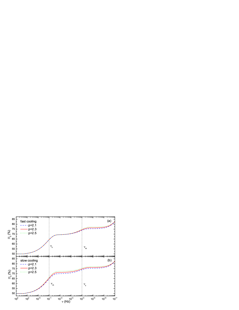
Figure 6: The dependence of $\Pi_{0}$ on the observed frequency $\nu$. Panel (a): the fast-cooling case ($\nu_{c}<\nu_{m}$); Panel (b): the slow-cooling case ($\nu_{c}>\nu_{m}$). The dashed, solid and dotted lines correspond to $p=2.1$, $2.3$, and $2.5$ respectively.

The above approaches are consistent with those in Table 1 of Granot (2003), in which the simple analytic expression for $\Pi_{0}$ as a function of the spectral slope for optically thin synchrotron emission can be found. Figure A1 clearly shows how the polarization degree $\Pi_{0}$ varies with the observed frequency $\nu=\delta(\gamma,\theta)(1+z)^{-1}\nu^{\prime}$. As can be seen, in both fast and slow cooling cases, there are three platforms in each polarization curve, which represent the three typical polarization levels discussed above.

References

- [] Barth A. J., et al., 2003, ApJ, 584, L47
- [] Berger E., et al., 2003, Nat, 426, 154
- [] Björnsson G., 2002, proceedings of the 1st Niels Bohr Summer Institute on Beaming and Jets in Gamma Ray Bursts, Copenhagen, Denmark, 12-30 Aug. 2002, eConf C0208122:66-72 (astro-ph/0302177)
- [] Björnsson G., Gudmundsson E. H., Jóhannesson G., 2004, ApJ, 615, L77
- [] Blandford R. D., McKee C. F., 1976, Phys. Fluids, 19, 1130
- [] Covino S., et al., 1999, AA, 348, L1
- [] Covino S., Ghisellini G., Lazzati D., Malesani D., 2002, in Feroci M., Masetti N., Piro, L. eds, ASP Conf. Ser. Vol. 312, Third Rome Workshop on Gamma Ray Bursts in the Afterglow Era, (astro-ph/0301608)
- [] Covino S., et al., 2003a, AA, 400, L9
- [] Covino S., et al., 2003b, AA, 404, L5
- [] Dai Z. G., Lu T., 1999, ApJ, 519, L155
- [] Dai Z. G., Gou L. J., 2001, ApJ, 552, 72
- [] Dai Z. G., Cheng K. S., 2001, ApJ, 558, L109
- [] Dai Z. G., 2004, ApJ, 606, 1000
- [] Frail D., et al., 2000, ApJ, 538, L129
- [] Ghisellini G., Lazzati D., 1999, MNRAS, 309, L7
- [] Gorosabel J., et al., 2004, AA, 422, 113
- [] Granot J., Panaitescu A., Kumar P., Woosley S., 2002, ApJ, 570, L61
- [] Granot J., Kumar P., 2003, ApJ, 591, 1086
- [] Granot J., Königl A., 2003, ApJ, 594, L83
- [] Granot J., 2003, ApJ, 596, L17
- [] Greiner J., et al., 2003, Nat, 426, 157
- [] Gruzinov A., Waxman E., 1999, ApJ, 511, 852
- [] Gruzinov A., 1999, ApJ, 525, L29
- [] Huang Y. F., Dai Z. G., Lu T., 2000, MNRAS, 316, 943
- [] Huang Y. F., Cheng K. S., 2003, MNRAS, 341, 263
- [] Huang Y. F., Wu X. F., Dai Z. G., Ma H. T., Lu T., 2004, ApJ, 605, 300
- [] Kumar P., Granot J., 2003, ApJ, 591, 1075
- [] Laing R. A, 1980, MNRAS, 193, 439
- [] Laursen L. T., Stanek K. Z., 2003, ApJ, 597, L107
- [] Lazzati D., et al., 2004, AA, 422, 121
- [] Li W. D., Filippenko A. V., Chornock R., Jha S., 2003, PASP, 115, 844
- [] Liang E. W., Dai Z. G., 2004, ApJ, 608, L9
- [] Loeb A., Perna R., 1998, ApJ, 495, 597
- [] Longair M. S., 1994, High Energy Astrophysics, Volume 2 (Cambridge University)
- [] Lyutikov M., Pariev V. I., Blandford R., 2003, ApJ, 597, 998
- [] Medvedev M. V., Loeb A., 1999, ApJ, 526, 697
- [] Mészáros P., Rees M., 1999, MNRAS, 306, L39
- [] Mészáros P., Rees, M., Wijers, R. A. M. J., 1998, ApJ, 499, 301
- [] Nakar E., Oren Y., 2004, ApJ, 602, L97
- [] Panaitescu A., Kumar P., 2000, ApJ, 543, 66
- [] Peng F., Königl A., Granot J., 2004, ApJ submitted (astro-ph/0410384)
- [] Rhoads J. E., 1999, ApJ, 525, 737
- [] Rol E., et al., 2000, ApJ, 544, 707
- [] Rol E., et al., 2003, AA, 405, L23
- [] Rossi E. M., Lazzati D., Rees M. J., 2002, MNRAS, 332, 945
- [] Rossi E. M., Lazzati D., Salmonson J. D., Ghisellini G., 2004, MNRAS, 354, 86
- [] Sari R., Piran T., Narayan R., 1998, ApJ, 497, L17
- [] Sari R., Piran T., Halpern J. P., 1999, ApJ, 519, L17
- [] Sari R., 1999, ApJ, 524, L43
- [] Sari R., Esin A. A., 2001, ApJ, 548, 787
- [] Waxman E., 1997, ApJ, 485, L5
- [] Wei D. M., Lu T., 1998, ApJ, 505, 252
- [] Wijers R. A. M. J., et al., 1999, ApJ, 523, L33
- [] Wu X. F., Dai Z. G., Liang E. W., 2004, ApJ, 615, 359
- [] Zhang B., Mészáros P., 2002, ApJ, 571, 876
- [] Zhang W., Woosley S. E., Heger A., 2004, ApJ, 608, 365