Inclusion of Binaries in Evolutionary Population Synthesis

Abstract

Using evolutionary population synthesis we present integrated colours, integrated spectral energy distributions and absorption-line indices defined by the Lick Observatory image dissector scanner (referred to as Lick/IDS) system, for an extensive set of instantaneous burst binary stellar populations with and without binary interactions. The ages of the populations are in the range $1-15\,$Gyr and the metallicities are in the range $0.0001-0.03$. By comparing the results for populations with and without binary interactions we show that the inclusion of binary interactions makes the integrated $\rm U-B$, $\rm B-V$, $\rm V-R$ and $\rm R-I$ colours and all Lick/IDS spectral absorption indices (except for $\rm H_{\beta}$) substantially smaller. In other words binary evolution makes a population appear bluer. This effect raises the derived age and metallicity of the population.

We calculate several sets of additional solar-metallicity binary stellar populations to explore the influence of input parameters to the binary evolution algorithm (the common-envelope ejection efficiency and the stellar wind mass-loss rate) on the resulting integrated colours. We also look at the dependence on the choice of distribution functions used to generate the initial binary population. The results show that variations in the choice of input model parameters and distributions can significantly affect the results. However, comparing the discrepancies that exist between the colours of various models, we find that the differences are less than those produced between the models with and those without binary interactions. Therefore it is very necessary to consider binary interactions in order to draw accurate conclusions from evolutionary population synthesis work.

1 Introduction

Amongst the distinct methods available for the study of the integrated light of stellar populations it is the evolutionary population synthesis (EPS) method (first introduced by Tinsley 1968) that offers the most direct approach for modelling galaxies. Remarkable progress in this field has been made during the past decades but the majority of EPS studies have tended to focus solely on the evolution of single stars (Bressan, Chiosi & Fagotto, 1994; Worthey, 1994; Vazdekis et al., 1996; Kurth, Alvensleben & Fricke, 1999).

Both observation and theory tell us that binary stars play a very important role in the evolution of stellar population. First, observations show that upwards of 50% of the stars populating galaxies are expected to be in binary or higher-order multiple systems (Duquennoy & Mayor, 1991; Richichi et al., 1994, for example). Secondly, binary evolution, if the component stars are close enough to exchange mass, can drastically alter the evolution path of a star as expected from single star evolution. Moreover, binary interactions can also create some important classes of objects such as blue stragglers (BSs: Pols & Marinus 1994), and subdwarf B stars (sdBs, also referred as extreme horizontal branch [EHB] stars: Han et al. 2002, 2003). These objects produced by binary evolution channels, can significantly affect the integrated spectral energy distribution (ISED) of a population from ultraviolet (UV) to radio ranges. Therefore it is necessary to include binary stars in EPS models. However, in the few EPS studies to date that have accounted for binary evolution, some only included specialised classes of binaries (for example, massive close binary evolution: Van Bever & Vanbeveren 1998, 2000), while others were limited to studying specialised stellar populations (e.g. Pols & Marinus 1994; Cerviño, Mas-Hesse & Kunth Cerviño et al.1997; Van Bever & Vanbeveren 1997, 2003). The EPS study of Zhang et al. (2004b, hereafter Paper I) took into account various known classes of binary stars and investigated general populations but they only considered solar metallicity populations. This paper expands that study by including a metallicity dependence and by investigating the effects of binary interactions and model input parameters on the results. Furthermore, by using $1\times 10^{6}$ instead of $2\times 10^{5}$ binary systems the error in the calculations is reduced and the solar metallicity results of Paper I are superceded.

In this paper we assume that all stars are born in binaries and born at the same time, i.e. an instantaneous binary stellar population (BSP). EPS models of instantaneous burst BSPs require four key ingredients: (i) a library of evolutionary tracks (including binary stars and single stars) used to calculate isochrones in the colour-magnitude diagram (CMD); (ii) a library of stellar spectra adopted in order to derive the ISED, or magnitudes and colours, in suitable passbands; (iii) a method to transform spectral information to absorption-line strengths, for example, the approach of empirical fitting polynomials (Worthey et al., 1994); and (iv) assumptions regarding the various distributions required for initialization of the binary population, such as the initial mass function (IMF) of the primaries and the distribution of orbital separations.

The outline of the paper is as follows: we describe our EPS models and algorithm in Section 2; our results are presented in Section 3 and in Section 4 we investigate the influences of binary interactions, model input parameters and distribution functions on the results; and then finally, in Section 5, we give our conclusions.

2 Model Description

The EPS code used here was developed by Zhang and colleagues (Zhang et al., 2002, 2004a, 2004b) and is based on the most updated input physics. Here we briefly describe the important features and components of the model as well as providing details of the algorithm for computing a BSP.

2.1 Initialization of the binary population

To investigate the effect of binary interactions on the EPS study of stellar populations we first need to construct the instantaneous burst BSPs. The evolution path taken by a star in a binary depends critically on the mass of the companion star and the orbital parameters. As such, binary evolution can be very complex and it is difficult to estimate the evolutionary timescales of the two stars without actually evolving the system. Therefore, the traditional method of constructing populations used in the EPS study of single stellar populations, where only the IMF need be considered and the evolutionary timescale of a star is set as soon as its mass is set, confronts difficulty in the study of BSPs. Here we need to use a Monte Carlo process, which utilises a random-number generator in combination with distribution functions, to generate the initial conditions of a set of binaries which then need to be evolved using an appropriate binary evolution model.

To generate a BSP the following input distributions are required to define the initial state of each binary: (i) the IMF of the primaries, which gives the relative number of the primaries in the mass range $M\rightarrow M+{\rm d}M$; (ii) the secondary-mass distribution; (iii) the distribution of orbital separations (or periods); and (iv) the eccentricity distribution. For distributions for which the majority of studies have reached fair agreement, such as the primary-mass and orbital separation distributions, we use a certain form while for those that are less constrained (secondary-mass and eccentricity) we use several reasonable assumptions. We also need to set the lower and upper mass cut-offs $M_{{\rm l}}$ and $M_{{\rm u}}$ to the mass distributions and assign a metallicity $Z$ to the stars.

For each binary system the initial mass of the primary is chosen from the approximation to the IMF of Miller & Scalo (1979) as given by Eggleton, Fitchett & Tout (1989, hereinafter EFT),

$$M_{1}={\frac{0.19X}{(1-X)^{0.75}+0.032(1-X)^{0.25}}}\,,$$ (1)

where $X$ is a random variable uniformly distributed in the range [0,1], and $M_{1}$ is the primary mass in units of ${\rm M_{\odot}}$.

In choosing the initial mass of the secondary star we can assume that the masses of the component stars are either correlated or that they are independent. For the correlated case, the secondary-mass distribution depends on the primary-mass (as set by equation 1) and the mass-ratio, $q$, distribution. The form of the latter is somewhat uncertain and a matter for debate. In this study we consider two versions of the $q$ distribution, one is a uniform distribution (EFT 1989; Mazeh et al., 1992; Goldberg & Mazeh, 1994),

$$n(q)=1,\ \ \ \ \ 0\leq q\leq 1,$$ (2)

where $q=M_{2}/M_{1}$, and the other is a thermal distribution (Han, Podsiadlowski & Eggleton, 1995),

$$n(q)=2q,\ \ \ \ \ 0\leq q\leq 1.$$ (3)

In the uncorrelated case, the secondary mass is chosen independently from the same IMF as the primary (equation 1).

The distribution of orbital separations is taken as constant in $\log a$ (where $a$ is the separation) for wide binaries and falls off smoothly at close separations:

$$an(a)=\Bigl{\{}\matrix{\ a_{\rm sep}(a/a_{0})^{m},&\ \ \ a\leq a_{0},\cr a_{\rm sep},\ \ \ \ \ \ \ \ \ &\ \ \ \ \ \ \ \ \ \ a_{0}<a<a_{1},\cr}$$ (4)

where $a_{\rm sep}\approx 0.070$, $a_{0}=10{\rm R_{\odot}}$, $a_{1}=5.75\times 10^{6}{\rm R_{\odot}}$ and $m\approx 1.2$. This distribution implies that there are equal numbers of wide binary systems per logarithmic interval, and that approximately 50% of the binary systems have orbital periods less than 100 yr. The value of 100 yr can be viewed as the upper limit for interaction between the component stars – if the period is longer than 100 yr the evolution of the stars does not differ from that of two independent single stars. This fraction of 50% for binaries with a period less than 100 yr is a typical value for the Galaxy, resulting in $\sim 10\%$ of the binaries experiencing Roche lobe overflow (RLOF) during the past 13 Gyr.

In order to investigate the effect of eccentricity we consider two eccentricity distributions: (i) all binaries are initially circular, i.e.

$$e=0\,,$$ (5)

and (ii) all binaries are formed in eccentric orbits where the initial eccentricity distribution satisfies a uniform form, i.e.,

$$e=X.$$ (6)

Under this second assumption large eccentricities in short-period orbits are to be excluded on the basis that the stars will crash into each other at periastron.

Equations (1) - (6) can be used to set the initial state of a binary system: the masses of the component stars, $M_{1}$ and $M_{2}$, separation, $a$, and eccentricity, $e$, of the orbit.

2.2 Binary evolution model and input parameters

To describe the evolution of a binary we use the rapid binary star evolution (BSE) algorithm of Hurley, Tout & Pols (2002). The BSE algorithm provides the stellar luminosity $L$, effective temperature $T_{\rm eff}$, radius $R$, current mass $M$ and the ratio of radius to Roche-lobe radius $R/R_{\rm L}$ for the component stars, as well as the period $P$, separation $a$ and eccentricity $e$ for a binary system. It is valid for component star masses in the range $0.1\leq M_{1},M_{2}\leq 100M_{\odot}$, metallicity $0.0001\leq Z\leq 0.03$, and eccentricity $0.0\leq e<1.0$. The BSE algorithm includes the single star evolution (SSE) package of analytic formulae as presented by Hurley, Pols & Tout (2000) in its entirety. In fact, for orbits that are wide enough that mass exchange between the component stars does not take place, the evolutionary parameters of the stars are identical to that given by the SSE package. The SSE package comprises a set of analytic evolution functions fitted to the model tracks of Pols et al. (1998). Detailed descriptions of the stellar evolutionary models of Pols et al. (1998) and the SSE package have been presented previously in Zhang et al. (2002: see Sec. 2), so we do not discuss them here. In addition to all aspects of single star evolution, the BSE algorithm models processes such as mass transfer, mass accretion, common-envelope (CE) evolution, collisions, supernova kicks, tidal evolution, and all angular momentum loss mechanisms. This is done mostly by using a prescription (or recipe) based approach.

For the BSE code there are several important input parameters that require mention:

• (i) the efficiency of CE ejection $\alpha_{{\rm CE}}$ in the CE evolution model denotes the fraction of the orbital energy that is transferred to the envelope and is used to overcome the binding energy. This efficiency is defined (Iben & Livio, 1993) by

  $$\alpha_{{\rm CE}}={\Delta E_{\rm bind}\over\Delta E_{\rm orb}},$$ (7)

  where $\Delta E_{\rm orb}$ is the change in the orbital energy of the binary between the initial and final state of the spiraling-in process and $\Delta E_{\rm bind}$ is the energy added to the binding energy of the envelope. If the envelope is ejected before complete spiral-in then a close binary is the result, otherwise the two stars will coalesce. This parameter is crucial in understanding the evolution of populations of binary systems because it determines the outcome of a CE interaction. In our BSP study we vary it over a reasonable range ($1.0-3.0$) to investigate its effects.

• (ii) the coefficient $\eta$ for Reimers’ wind mass-loss (Reimers, 1975),

  $$\dot{M}_{\rm R}=4\times 10^{-13}\eta\frac{LR}{M}M_{\odot}{\rm yr^{-1}},$$ (8)

  where stellar luminosity, $L$, radius, $R$, and mass $M$, are all in solar units. Equation (8) gives the wind mass-loss rate for intermediate and low-mass stars on the giant branch and beyond. In this study we vary $\eta$ from 0.5 to 0.0.

• (iii) the tidal enhancement parameter $B$, which appears in the formula of tidally enhanced mass loss given by Tout & Eggleton (1988),

  $$\dot{M}=\dot{M}_{\rm R}\Big{[}1+B_{\rm W}{\rm max}\big{(}{1\over 2},{R\over R_{\rm L}}\big{)}^{6}\Big{]}$$ (9)

  where $\dot{M}_{\rm R}$ is the Reimers’ rate (see equation 8) and $R_{\rm L}$ is the Roche lobe radius. Equation (9) is used to increase the incidence of RS CVn binaries. In this study we do not consider tidally enhanced mass loss, i.e., $B=0.0$.

2.3 Stellar spectra and absorption line indices

The BaSeL-2.0 stellar spectra library of Lejeune et al. (1997, 1998) provides an extensive and homogeneous grid of low-resolution theoretical flux distributions in the range of $9.1-160000\,$nm, and synthetic UBVRIJHKLM colours for a large range of stellar parameters: $2000\leq T_{{\rm eff}}/{\rm K}\leq 50000$, $-1.02\leq\log g\leq 5.50$, and $+1.0\leq{\rm[Fe/H]}\leq-5.0$ (where $g$ denotes surface gravity). For this library correction functions have been calculated for each value of the $T_{{\rm eff}}$ and for each wavelength in order to yield synthetic UBVRIJHKLM colours matching the empirical colour-$T_{{\rm eff}}$ calibrations derived from observations at solar metallicity. Semi-empirical calibrations for non-solar abundances ($\rm[Fe/H]=-3.5$ to +1.0) have also been established for this version of the library. After correction the most important systematic differences existing between the original model spectra and the observations are eliminated. Furthermore, synthetic UBV and Washington ultraviolet excesses $\delta_{\rm(U-B)}$, $\delta_{\rm(C-M)}$ and $\delta_{\rm(C-T_{1})}$, obtained from the original model spectra of giants and dwarfs, are in excellent agreement with the empirical metal-abundance calibrations.

The empirical fitting functions of Worthey et al. (1994) give absorption-line indices defined by the Lick Observatory image dissector scanner (Lick/IDS) system as a function of $T_{{\rm eff}}$, $\log g$, and metallicity [Fe/H]. The effective temperature spans a range of $2100\leq T_{{\rm eff}}/{\rm K}\leq 11000$ and the metallicity is in the range $-1.0\leq{\rm[Fe/H]}\leq+0.5$. The indices in the Lick system were extracted from the spectra of 460 stars obtained between 1972 and 1984 using the red-sensitive IDS and Cassegrain spectrograph on the 3m Shane telescope at Lick Observatory. The spectra cover the range $4000-6400$ Å, with a resolution of $\sim 8$ Å (Worthey et al., 1994). A more detailed description of the Lick/IDS spectral absorption-feature indices has been presented in Zhang et al. (2004a: see Sec. 2).

2.4 The EPS algorithm

After choosing a seed for the random number generator we use the Monte Carlo eqns (1) - (6) to produce a population of $1\times 10^{6}$ binary systems. In this work the lower and upper mass cut-offs $M_{{\rm l}}$ and $M_{{\rm u}}$ are taken as 0.1 $\rm M_{\odot}$ and 100 $\rm{}^{M}_{\odot}$, respectively. The relative age, $\tau$, of the BSP is assigned within the range of $1-15\,$Gyr and the metallicity is chosen within the limits $0.0001\leq Z\leq 0.03$. We can then use the BSE algorithm to evolve each binary in the BSP to an age of $\tau$ which gives us evolutionary parameters such as $L$, $T_{\rm eff}$, $R$ and $M$ for the component stars. Next we use the BaSeL-2.0 stellar spectra to transform the evolutionary parameters to colours and stellar flux and then use the empirical fitting functions of Worthey et al. (1994) to derive spectral absorption feature indices in the Lick/IDS system. Finally, by the following equations (10) - (13) we can obtain the integrated colours, monochromatic flux and absorption feature indices for an instantaneous BSP of a particular age and metallicity. We note that the common-envelope phase of binary evolution is assumed to be instantaneous in the BSE algorithm and thus it is not a factor when calculating the flux. Other aspects of binary evolution that may affect the observed flux, such as the presence of an accretion disc or novae eruptions, are also not taken into account, i.e. we only consider the stellar parameters.

In the following equations, a parameter identified by a capital letter on the left-hand side represents the integrated BSP, while the corresponding parameter in minuscule on the right-hand side is for the $k-$th star. The integrated colour is expressed by

$$(C_{{\rm i}}-C_{{\rm j}})_{\tau,Z} =-2.5 \log{\frac{\sum_{{\rm k=1}}^{{\rm n}}\ 10^{-0.4c_{{\rm i}}}}{\sum_{{\rm k=1}}^{{\rm n}}\ 10^{-0.4c_{{\rm j}}}}}$$ (10)

where $c_{{\rm i}}$ and $c_{{\rm j}}$ are the $i$-th and $j$-th magnitude of the $k$-th star.

The integrated monochromatic flux of a BSP is defined as

$$F_{\lambda,\tau,Z}=\sum_{{\rm k=1}}^{{\rm n}}\ f_{\lambda},$$ (11)

where $f_{\lambda}$ is the SED of the $k$-th star.

The integrated absorption feature index of the Lick/IDS system is a flux-weighted one. For the $i-$th atomic absorption line, it is expressed in equivalent width ($W$, in Å),

$$W_{i,\tau,Z}={\frac{\sum_{{\rm k=1}}^{{\rm n}}\ w_{{\rm i}}\ \cdot f_{i,{\rm C}\lambda}}{\sum_{{\rm k=1}}^{{\rm n}}\ f_{i,{\rm C}\lambda}}},$$ (12)

where $w_{{\rm i}}$ is the equivalent width of the $i-$th index of the $k$-th star, and $f_{i,{\rm C}\lambda}$ is the continuum flux at the midpoint of the $i-$th ‘feature’ passband; and for the $i-$th molecular line, the feature index is expressed in magnitude,

$$C_{i,\tau,Z}=-2.5\log{\frac{\sum_{{\rm k=1}}^{{\rm n}}\ 10^{-0.4c_{{\rm i}}}\cdot\ f_{i,{\rm C}\lambda}}{\sum_{{\rm k=1}}^{{\rm n}}\ f_{i,{\rm C}\lambda}}},$$ (13)

where $c_{{\rm i}}$ is the magnitude of the $i-$th index of the $k$-th star (as in equation  10).

3 Results

Figure 1: The effects of binary interactions on $\rm U-B$ colour for BSPs of various metallicity. The symbols linked by line are for BSPs with binary interactions (Model A’) and those without a line are without binary interactions (Model B’). Different symbols denote different metallicities, from top to bottom, the metallicity $Z$ is 0.03, 0.02, 0.01, 0.004, 0.001, 0.0003 and 0.0001, respectively.

Figure 2: Similar to Fig. 1 but for $\rm B-V$ colour.

Figure 3: The fractional contributions of different evolutionary stages to the total flux are shown for solar metallicity BSPs at an age of 1  Gyr. Top and bottom panels are for Models A’ and B’, respectively. The abbreviations are explained in the text.

Figure 4: Similar to Fig. 3 but for an age of 13  Gyr.

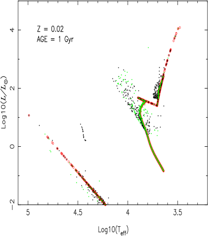
Figure 5: Theoretical isochrones for solar-metallicity instantaneous burst BSPs at an age of 1 Gyr. Open circles for Model B’, dots for Models A’ (black for the primary, blue for the secondary). For the sake of clarity only $1\times 10^{5}$ binary systems are included and those MS stars with mass $M\la 0.7{\rm M_{\odot}}$ are removed. All binaries are assumed to be resolved.

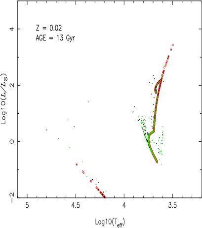
Figure 6: Similar to Fig. 5 but for an age of 13  Gyr.

Table 1: The integrated colours for Model A’.

Age	1.00	2.00	3.00	4.00	5.00	6.00	7.00	8.00	9.00	10.00	11.00	12.00	13.00	14.00	15.00
(Gyr)
$Z$ = 0.0001
$\rm U-B$	-0.021	-0.001	0.009	0.018	-0.009	-0.006	-0.007	0.005	0.007	-0.012	0.007	-0.004	0.002	-0.010	-0.018
$\rm B-V$	0.266	0.404	0.484	0.547	0.515	0.554	0.553	0.569	0.579	0.534	0.573	0.574	0.580	0.587	0.572
$\rm V-R$	0.274	0.339	0.382	0.408	0.366	0.386	0.389	0.401	0.404	0.373	0.400	0.403	0.410	0.411	0.399
$\rm V-I$	0.647	0.755	0.829	0.870	0.781	0.816	0.824	0.846	0.853	0.790	0.841	0.849	0.861	0.861	0.838
$Z$ = 0.0003
$\rm U-B$	-0.063	0.011	0.015	0.025	0.011	-0.008	-0.011	-0.030	-0.010	0.004	0.007	0.010	0.046	0.030	0.032
$\rm B-V$	0.295	0.431	0.518	0.583	0.593	0.625	0.631	0.607	0.654	0.667	0.666	0.654	0.691	0.651	0.646
$\rm V-R$	0.271	0.350	0.395	0.427	0.407	0.425	0.431	0.406	0.435	0.448	0.441	0.439	0.470	0.442	0.437
$\rm V-I$	0.627	0.781	0.855	0.911	0.856	0.885	0.899	0.841	0.898	0.922	0.909	0.911	0.970	0.916	0.904
$Z$ = 0.001
$\rm U-B$	-0.038	0.045	0.076	0.065	0.070	0.068	0.051	0.050	0.033	0.045	0.073	0.038	0.058	0.062	0.108
$\rm B-V$	0.343	0.463	0.577	0.632	0.663	0.679	0.692	0.712	0.688	0.692	0.727	0.677	0.658	0.678	0.664
$\rm V-R$	0.303	0.360	0.401	0.437	0.440	0.445	0.449	0.470	0.448	0.448	0.473	0.440	0.431	0.441	0.446
$\rm V-I$	0.696	0.821	0.872	0.952	0.934	0.930	0.931	0.974	0.925	0.920	0.969	0.908	0.887	0.908	0.929
$Z$ = 0.004
$\rm U-B$	0.077	0.116	0.102	0.134	0.164	0.198	0.211	0.192	0.221	0.242	0.257	0.253	0.275	0.275	0.273
$\rm B-V$	0.366	0.544	0.624	0.692	0.730	0.775	0.790	0.772	0.803	0.824	0.833	0.819	0.833	0.844	0.838
$\rm V-R$	0.281	0.356	0.401	0.430	0.449	0.471	0.483	0.476	0.482	0.495	0.501	0.507	0.511	0.514	0.509
$\rm V-I$	0.689	0.808	0.891	0.920	0.959	0.990	1.034	1.020	1.001	1.026	1.049	1.081	1.065	1.074	1.055
$Z$ = 0.01
$\rm U-B$	0.139	0.147	0.198	0.237	0.275	0.308	0.305	0.348	0.372	0.384	0.394	0.408	0.433	0.443	0.458
$\rm B-V$	0.443	0.642	0.723	0.757	0.784	0.829	0.825	0.859	0.881	0.885	0.888	0.893	0.903	0.911	0.917
$\rm V-R$	0.295	0.399	0.439	0.457	0.471	0.493	0.491	0.507	0.518	0.522	0.521	0.525	0.529	0.529	0.537
$\rm V-I$	0.704	0.890	0.936	0.980	0.991	1.033	1.024	1.047	1.067	1.082	1.080	1.081	1.091	1.089	1.111
$Z$ = 0.02
$\rm U-B$	0.167	0.204	0.289	0.351	0.396	0.438	0.487	0.480	0.512	0.587	0.587	0.618	0.639	0.642	0.705
$\rm B-V$	0.525	0.696	0.788	0.839	0.878	0.905	0.938	0.919	0.960	0.990	0.998	0.981	1.022	1.029	1.037
$\rm V-R$	0.322	0.422	0.469	0.491	0.510	0.523	0.541	0.536	0.554	0.566	0.570	0.559	0.577	0.565	0.586
$\rm V-I$	0.704	0.889	0.985	1.006	1.052	1.071	1.109	1.092	1.135	1.165	1.168	1.129	1.166	1.160	1.186
$Z$ = 0.03
$\rm U-B$	0.183	0.278	0.355	0.415	0.470	0.495	0.518	0.557	0.648	0.675	0.700	0.761	0.820	0.820	0.829
$\rm B-V$	0.570	0.748	0.820	0.875	0.908	0.936	0.947	0.980	1.015	1.012	1.018	1.055	1.091	1.086	1.077
$\rm V-R$	0.346	0.444	0.490	0.522	0.537	0.556	0.562	0.584	0.598	0.591	0.599	0.609	0.625	0.623	0.619
$\rm V-I$	0.734	0.901	1.002	1.069	1.075	1.117	1.121	1.181	1.220	1.187	1.198	1.217	1.237	1.255	1.254

In this part we present integrated colours, ISEDs at intermediate resolution (10 Å  in the UV and 20 Å  in the visible) and Lick/IDS absorption feature indices for instantaneous burst BSPs with and without binary interactions over a large range of age and metallicity: $1\leq\tau\leq 15$ Gyr and $-2.3\leq{\rm[Fe/H]}\leq+0.2$. For each model, a total of $1.0\times 10^{6}$ binaries are evolved according to the algorithm given in the previous section.

3.1 Colours

In Table 1 we present $\rm U-B$, $\rm B-V$, $\rm V-R$ and $\rm V-I$ colours for the set of BSPs that we call Model A’. In this model binary interactions are included by utilizing the BSE algorithm, the initial mass of the secondary $M_{2}$ is assumed to be correlated with $M_{1}$ and is obtained from a uniform mass-ratio distribution (see equation 2), eccentric orbits are allowed for the binary systems and a uniform eccentricity distribution is adopted (see equation 6), the CE ejection efficiency $\alpha_{\rm CE}$ is set to 1.0, and the Reimers’ wind mass-loss coefficient $\eta$ is 0.3. The model is repeated for seven distinct values of Z: 0.03, 0.02, 0.01, 0.004, 0.001, 0.0003 and 0.0001, respectively.

To investigate the effect of binary interactions on the results, we also construct Model B’, which differs from Model A’ by neglecting all binary interactions, i.e. the component stars are evolved as if in isolation according to the SSE algorithm. In Figs 1 and 2 we give a comparison of the integrated $\rm U-B$ and $\rm B-V$ colours for Models A’ (generated from Table 1) and B’. We see that the inclusion of binary interactions makes the integrated $\rm U-B$ and $\rm B-V$ colours of various metallicity BSPs bluer for all instances.

In Figs 3 and 4 we give the fractional contribution of different evolutionary stages to the total flux for solar metallicity $1-$ and 1$3-$Gyr BSPs, respectively. The top panels of Figs 3 and 4 are for Model A’, while the bottom panels are for Model B’. In each of them various abbreviations are used to denote the evolution phases. They are as follows: ’MS’ stands for main-sequence stars, which are divided into two phases to distinguish deeply or fully convective low-mass stars ($M\la 0.7\rm{M_{\odot}}$, therefore Low-MS) and stars of higher mass with little or no convective envelope ($M\ga 0.7\rm{M_{\odot}}$); ’HG’ stands for Hertzsprung gap; ’GB’ stands for the first giant branch; ’CHeB’ stands for core helium burning; ’EAGB’ stands for early asymptotic giant branch stars; ’PEAGB’ (post EAGB) refers to those phases beyond the ’EAGB’ – including thermally pulsing giant branch/proto planetary nebula/planetary nebula (TPAGB/PPN/PN); ’HeMS’ stands for helium star main-sequence; ’HeHG’ stands for helium star Hertzsprung gap; ’HeGB’ stands for helium star giant branch; and ’HeWD’ and ’COWD’ stand for helium and carbon/oxygen white dwarfs, respectively. Correspondingly, in Figs 5 and 6 we plot theoretical isochrones of solar metallicity $1-$ and $13-$Gyr BSPs. Note that all stars except for Low-MS stars are included in the isochrones.

Comparing the contribution of different evolutionary stages to the total flux between Model A’ and Model B’ for solar metallicity 1- Gyr BSPs (Fig. 3), we find that the flux in the UBVRI passbands is dominated by the same evolutionary stages regardless of model. This is also true for the $13\,$Gyr solar metallicity BSPs (Fig. 4). For the young BSPs the UBVRI flux is dominated by MS stars with mass $M\ga 0.7{\rm M_{\odot}}$, CHeB stars and cooler PEAGB (in fact the TPAGB) stars. MS and CHeB stars also dominate for the old BSPs but here the GB stars make a major contribution as well. Therefore, the differences in the integrated ${\rm U-B},{\rm B-V},{\rm V-R}$ and ${\rm V-I}$ colours between Model A’ and Model B’ will originate from differences in the distribution of these classes of stars which dominate the total UBVRI flux. From Figs 5 and 6 we see clearly that the distribution of stars in the Hertzsprung-Russell (HR) diagram for Model A’ is significantly different from that of Model B’. The distribution of the stars is more dispersed for Model A’ in comparison with Model B’ and, as you would expect, BS stars are produced only by Model A’. Moreover, for young BSPs, Fig. 5 shows that Model A’ produces a lot of scatter around the MS as well as hotter CHeB stars compared to Model B’. For old BSPs, Fig. 6 shows that Model A’ also produces MS, GB and CHeB stars which differ from the corresponding class of stars in Model B’. The net effect of the difference in the distribution of these classes of stars is to make the populations hotter and therefore Model A’ appears younger when compared with Model B’.

So far we have neglected to discuss redder colours (such as, $\rm J-K$, $\rm H-K$, etc) and the reason is their relatively large errors. From the top and bottom panels of Fig. 3, we see that cooler PEAGB stars ($T_{\rm eff}\la 3.54$, see Fig. 5) give the maximal contribution to the total flux in those redder passbands for young BSPs. The evolutionary timescale of these PEAGB stars is so short compared with that of MS stars that there are few PEAGB stars in our $1\times 10^{6}$ binary system sample. Therefore, for young BSPs large error can result from fluctuations in the small number of PEAGB stars and thus, the evolutionary curves of these colours are not smooth. For old BSPs, from the top and bottom panels of Fig. 4 we see that GB stars contribute about 50% of the total flux in the redder wavelength range: in fact, it is GB stars with temperature $T_{\rm eff}\la 3.54$ that give the maximal contribution. Although the evolutionary timescale of these stars is longer than that of young PEAGB stars it is still relatively short compared to the age of the population and once again a large error can be introduced in the red flux range. The reason we focus on the bluer colours is that the total flux in the UVBRI passbands is dominated by stars which have long evolutionary timescales and the error here is comparitively small.

3.2 The integrated spectral energy distribution

Figure 7: The integrated spectral energy distributions as a function of age for solar-metallicity BSPs with binary interactions (Model A’). From top to bottom, the ages are $\tau=1,2,4,7,10$ and 15  Gyr, respectively. The flux is expressed in magnitudes and is normalized to zero at 2.2 $\mu$m.

Figure 8: The integrated spectral energy distributions as a function of metallicity for BSPs with binary interactions (Model A’) at age $\tau=10$  Gyr. From bottom to top, the metallicity $Z$ is 0.0001, 0.0003, 0.001, 0.004, 0.01, 0.02 and 0.03, respectively. The flux is also expressed in magnitudes and is normalized to zero at 2.2 $\mu$m.

Figure 9: The integrated spectral energy distributions for solar metallicity instantaneous BSPs with (full line) and without (dashed line) binary interactions at ages $\tau=1,2,4,7,10$ and 15  Gyr (from top to bottom, respectively). For Models A’ arrows mark the blue end at which MS stars with mass $M\la 0.7{\rm M_{\odot}}$ contribute 10% of the ISED, and for Model B’ we do not plot flux shorter than this point. Note for young BSPs the blue end where MS stars with mass $M\la 0.7{\rm M_{\odot}}$ give a 10% contribution is significantly different for Models A’ and B’, while for old BSPs this discrepancy is insignificant. For the sake of clarity the fluxes at ages of $2,4,7,10,15$ Gyr are shifted downwards by an mount of -4.0.

In Figs 7 and 8 we give the variation of the intermediate-resolution ISED with age and metallicity over a wide wavelength range, $2.7\leq\log\lambda/{\rm\AA}\leq 5.2$, for Model A’. The flux is expressed in magnitudes and is normalized to zero at 2.2 $\mu$m. Figs 7 and 8 show that the effects of age and metallicity on the ISEDs are similar, i.e. the ISEDs tend to be redder with increasing age and metallicity in the wavelength region $3.3\leq\log\lambda/{\rm\AA}\leq 4.2$.

In Fig. 9 we compare the ISEDs of Model A’ with those of Model B’ for solar-metallicity BSPs at ages $\tau=1,2,4,7,10$ and 15 Gyr (note that the ISEDs for Model A’ have also been given in Fig. 7). In Fig. 9, for Model A’ arrows mark the blue end ($\lambda_{1,\tau}$) at which MS stars with mass $M\ga 0.7{\rm M_{\odot}}$ give a 10% contribution to the total flux. For Model B’ we do not give the fluxes shorter than the wavelength $\lambda_{2,\tau}$ (defined as for $\lambda_{1,\tau}$ but for Model B’). Note that for young BSPs $\lambda_{1,\tau}$ of Model A’ is significantly different from $\lambda_{2,\tau}$ of Model B’, with $\lambda_{1,\tau}<\lambda_{2,\tau}$, while for old BSPs we find $\lambda_{1,\tau}\approx\lambda_{2,\tau}$. The differences between $\lambda_{1,\tau}$ and $\lambda_{2,\tau}$ are explained by the absence of BS stars in Model B’, while in Model A’ the number of hot BS stars at early ages is greater than at old ages. Fig. 9 shows significant disagreement of the ISED between Model A’ and Model B’ in the UV and far-UV regions ($\log\lambda/{\rm\AA}\la 3.4$): the ISED for Model A’ is bluer than that for Model B’ at all ages. Comparing this discrepancy for the young and old BSPs it seems that it decreases with age: at $\tau=1$ Gyr the discrepancy reaches to $\sim$ 5.0 mag at $\log\lambda/{\rm\AA}=3.1$ while at $\tau=15$ Gyr it decrease to $\sim$ 2.2 mag at $\log\lambda/{\rm\AA}=3.3$.

To aid investigation of the differences in the ISED in the UV and far-UV regions between Model A’ and Model B’ we have included arrows to mark the wavelength corresponding to $\lambda_{1,\tau}$ (left) and $\lambda_{2,\tau}$ (right) in Figs 3 and 4. For young $\tau=1$ Gyr BSPs, Fig. 3 shows that the ISED in the region of $\lambda_{2,\tau}\leq\log\lambda/{\rm\AA}\la 3.4$ is dominated by MS stars with mass $M\ga 0.7{\rm M_{\odot}}$ for both Model A’ and Model B’, and the fractional contribution of these MS stars drops from 0.93 to 0.1 rapidly at $\lambda_{2,\tau}$ for Model B’. So the discrepancy of the ISED in this region is mainly introduced by the difference in the distribution of MS stars with mass $M\ga 0.7{\rm M_{\odot}}$ (see Fig. 5). In the region $\lambda_{1,\tau}\leq\lambda\leq\lambda_{2,\tau}$ the total flux is mainly dominated by hotter PEAGB and/or CHeB stars for Model B’, while still by MS stars with mass $M\ga 0.7{\rm M_{\odot}}$ for Model A’, so the discrepancy in this region is mainly caused by the existence in Model A’ of more hot BSs. This analysis of the $\tau=1\,$Gyr BSP is also suitable for the $\tau=2,4,7,10$ Gyr BSPs. For the old $\tau=15$ Gyr BSP, $\lambda_{1,\tau}$ is almost equal to $\lambda_{2,\tau}$ and in this case the discrepancy of the ISED in the UV and far-UV regions is caused mainly by the difference in the distributions of MS stars with mass $M\ga 0.7{\rm M_{\odot}}$, hotter PEAGB and/or CHeB stars (as exhibited in Fig. 6).

For the young BSPs ($\tau=1$ and 2 Gyr) we also see some evidence in Fig. 9 of a disagreement of the ISEDs for Models A’ and B’ in the visible and infrared regions ($3.5\la\log\lambda/{\rm\AA}\la 4.0$). It appears that Model A’ exhibits a bluer continuum than Model B’ in this range and we believe this is owing to fluctuations introduced by the small number of cool PEAGB stars which, as discussed in Sec. 3.1, can make a significant contribution to the flux of young populations.

3.3 Lick spectral absorption feature indices

Figure 10: The effects of binary interactions on absorption-line indices in the Lick/IDS system for BSPs of various metallicity. The symbols linked by a line are for BSPs with binary interactions (Model A’), those without a line are for BSPs without binary interactions (Model B’). Different symbol denotes different metallicity, from top to bottom, the metallicity $Z$ is 0.03, 0..004, 0.001, 0.0003 and 0.0001, respectively.

In Table LABEL:licktab we present all resulting Lick/IDS spectral absorption feature indices for Model A’ for the seven metallicities we have considered. In Fig. 10 we show the corresponding evolutionary curves. We see that all indices except for ${\rm H}_{\beta}$ increase with increasing age and metallicity, with greater variation at early ages. For comparison, in Fig. 10 we also give Lick/IDS indices for Model B’. This comparison shows that all resulting Lick/IDS indices with binary interactions are bluer than those without binary interactions and it appears that these changes in Lick indices due to binaries, are very small compared to the typical changes with age and metallicity. The reason that the inclusion of binary interactions makes all resulting Lick/IDS spectral absorption feature indices bluer is that all of the indices are within the wavelength region of 4000 to 6400 Å, and in this region the ISED for Model A’ is bluer than that for Model B’ (see Fig. 9).

4 Influence of binary interactions, input parameters/distributions

Table 2: Model Parameters.

Model	BIs		$e$	$\alpha_{\rm CE}$		$\eta$	$n(q)$	$Z$
A	ON		E	1.0		0.3	CC	0.02
B	OFF		E	1.0		0.3	CC	0.02
C	ON		C	1.0		0.3	CC	0.02
D	ON		E	3.0		0.3	CC	0.02
E1	ON		E	1.0		0.0	CC	0.02
E2	ON		E	1.0		0.5	CC	0.02
F1	ON		E	1.0		0.3	UN	0.02
F2	ON		E	1.0		0.3	CQ	0.02

Figure 11: Difference of $\rm U-B$ colour between Model A and the other models (B-F).

Figure 12: Similar to Fig. 11 but for $\rm B-V$ colour.

We have performed six additional sets of Monte Carlo simulations in order to understand the effects of varying the model input parameters and initial distributions on the resulting U-B and B-V colours. Here we focus only on solar metallicity BSPs. The parameters we consider are the CE ejection efficiency $\alpha_{\rm CE}$ and the Reimers’ wind mass-loss coefficient $\eta$. The input distributions we vary are the eccentricity distribution and the initial mass distribution of the secondaries.

Each model differs from the other by changing one of the parameters or distributions used for the initial conditions of the BSP. The characteristics of each model are summarized in Table 2 where: the first column is the name of each model; the second column denotes the condition that binary interactions (BIs) are taken into account; the third column gives the eccentricity distribution, where ’E’ means all binaries are formed in eccentric orbits and the eccentricity satisfies a uniform distribution (see equation 6) and ’C’ denotes initially circular orbits (see equation 5); the fourth and fifth columns give the values of $\alpha_{\rm CE}$ and $\eta$; the sixth indicates the initial mass distribution of the secondaries, where ’CC’ represents the case that secondary-mass $M_{\rm 2}$ is correlated with primary-mass $M_{\rm 1}$ and the mass-ratio distribution $n(q)$ satisfies a constant form (see equation 2), ’CQ’ represents the correlated and thermal distribution case (see equation 3), and ’UN’ is for the uncorrelated case; and the last column gives the metallicity $Z$ (solar in all cases).

Our standard is Model A which is Model A’ restricted to solar metallicity. Similarly Model B is Model B’ restricted to only solar metallicity. For Model C binary interactions are taken into account but all binary orbits are initially circular. Model D is the same as Model A except that $\alpha_{\rm CE}=3.0$. Model E1 does not include any stellar wind ($\eta=0.0$) while in Model E2 $\eta=0.5$. To investigate the changes produced by altering the initial secondary-mass distribution Model F1 chooses the secondary-mass independently from the same IMF as used for the primary while in Model F2 the secondary-mass is correlated with primary-mass and the mass-ratio satisfies a thermal distribution.

To discuss the effects of binary interactions and the input parameters/distributions on the appearance of BSPs we use the difference of the integrated colours ($\Delta({\rm U-B})_{j-{\rm A}}$ and $\Delta({\rm B-V})_{j-{\rm A}}$) obtained by subtracting the colour for Model A from that of Model $j$ ($j=\,$B-F). All results for Model A have been given in Section 3 and the differences are plotted in Figs 11 and 12.

4.1 Binary interaction (Model B)

Binary stars play a very important role in EPS studies and as we pointed out earlier the majority of current EPS studies have only included single star evolution. In Section 3 we have already discussed the effect of the modelling of binary interactions on the integrated colours, ISED and Lick/IDS absorption line indices of a population for a range of metallicities. From the comparison of the integrated $\rm U-B$ and $\rm B-V$ colours for Models A and B in Figs 11 and 12 we see that the colours for Model A are less than those for Model B in almost all instances (the exception is $\rm B-V$ at 13 Gyr), i.e. for both colours considered the solar metallicity BSPs including binary interactions are bluer than those without binary interactions. For the full metallicity range ($Z=0.0001,0.003,0.001,0.004,0.01$ and 0.03) Figs 1 and 2 show that binary interactions play the same effect on $\rm U-B$ and $\rm B-V$ colours. Also Fig. 10 shows that binary interactions make all Lick/IDS absorption line indices bluer for BSPs regardless of metallicity. The reason that binary interactions make the integrated $\rm U-B$ and $\rm B-V$ colours and the Lick/IDS absorption indices bluer has been discussed in Section 3 and we do not take it further here.

4.2 The distribution of orbital eccentricity (Model C)

Figure 13: The total flux and the the fluxes of all MS stars with mass $M\ga 0.7{\rm M_{\odot}}$, CHeB and GB stars for Models A (full line) and C (dotted line) at an age of 1 Gyr. Each flux is expressed in units of the total flux at 2.2 $\mu$m ($F_{{\rm\lambda,2.2}\mu{\rm m}}$) for the corresponding model.

Figure 14: Similar to Fig. 13 but for an age of 13  Gyr.

Observations of binary stars show that the two components of the binary often move in eccentric orbits and that there are some systems for which the eccentricity approaches unity. Thus it would be wrong to neglect eccentricity when modelling binary evolution and accordingly Hurley et al. (2002) included eccentric orbits in their BSE algorithm. Statistical studies for the distribution of orbital eccentricity of binaries have found that it appears to be roughly uniform in the range from zero to unity (see equation 6), at least for those binaries whose components are sufficiently well separated that they can have had little chance yet to interact with each other, even at periastron (Eggleton, Han & Kiseleva-Eggleton, 2004). So in our standard model (Model A) we assumed that all binaries are formed with an eccentricity drawn from an uniform eccentricity distribution. However, to give an idea of how sensitive the integrated $\rm U-B$ and $\rm B-V$ colours are to changes in this distribution in Model C we consider the rather drastic case that all binaries are initially circular initially.

In Figs 11 and 12 we present the differences in the integrated $\rm U-B$ and $\rm B-V$ colours between Model C and Model A, i.e. $\Delta(\rm U-B)_{(C-A)}$ and $\Delta(\rm B-V)_{(C-A)}$. Fig. 11 shows that the integrated $\rm U-B$ colour for Model C is greater than that for Model A at most ages (except at $\tau=1,9$ and 15 Gyr), which means that if all binaries are in circular orbits the resulting $\rm U-B$ colour is redder, and thus, the populations appear older. In Fig. 12 a similar effect on the integrated $\rm B-V$ colour appears except at $\tau=1,9,13-15$ Gyr.

Why does Model C make the integrated $\rm U-B$ and $\rm B-V$ colours redder? In the BSE algorithm tidal interactions are modelled (circularisation and synchronisation) which means that an eccentric orbit may be circularised, if the stars are close enough for tides to become strong, and the orbital separation decreased. Now consider a binary in Model C which has a circular orbit and a separation $a$ such that mass-transfer is just avoided. The same binary in Model A with an initial eccentricity will experience tidal circularisation (most likely when the primary star reaches the GB) which will decrease $a$ and lead to mass-transfer. Also, closer systems that would initiate mass-transfer in Model C but not merge now are likely to lead to coalescence in Model A. In summary, the variation of the eccentricity distribution not only can influence the evolutionary path of close binaries but also that of relatively wide ones.

For binary populations, the variation in evolutionary path of binaries will cause variations in the number of stars and the distribution of stars in the CMD for different evolutionary phases. These two effects determine the discrepancies in the integrated colours and ISEDs. Because it is extremely difficult to describe the variation of the distribution of stars in the CMD we will focus only on the variation of the numbers of MS stars with mass $M\ga 0.7{\rm M_{\odot}}$, CHeB stars and GB stars. The reason is that the ISED in the UBV passbands is mainly contributed by these three evolutionary phases for both young (although GB stars do not contribute so strongly) and old BSPs (see Figs 3 and 4). For $\tau=1$ Gyr BSPs we find that: (i) on the MS the number of primaries with mass $M\ga 0.7{\rm M_{\odot}}$ for Model C is less than that for Model A (i.e., $\Delta N_{\rm p,MS,(C-A)}<0$) while that of secondaries with mass $M\ga 0.7{\rm M_{\odot}}$ for Model C is greater (i.e., $\Delta N_{\rm s,MS,(C-A)}>0$) and the decrease in the number of primaries is less than the increase in the number of secondaries (i.e., $\Delta N_{\rm p,MS,(C-A)}+\Delta N_{\rm s,MS,(C-A)}>0$); (ii) on the GB both the numbers of primaries and secondaries almost do not vary; and (iii) during CHeB the number of primaries for Model C is less than that for Model A ($\Delta N_{\rm p,CHeB,(C-A)}<0$) while the number of secondaries is greater ($\Delta N_{\rm s,CHeB,(C-A)}>0$) and $\Delta N_{\rm p,CHeB,(C-A)}\approx\Delta N_{\rm s,CHeB,(C-A)}$. For $\tau=13$ Gyr BSPs on the MS and GB both the numbers of primaries and secondaries for Model C are greater than those for Model A, while the opposite holds during CHeB.

In Figs 13 and 14 we give the total flux and the fluxes of all MS stars with mass $M\ga 0.7{\rm M_{\odot}}$, CHeB stars and GB stars over a wavelength range, $4000\leq\lambda\leq 10000{\rm\AA}$, for Models A and C at ages of 1 Gyr and 13 Gyr, respectively. Each flux curve is expressed in units of the total flux at 2.2 $\mu$m (i.e., $F_{{\rm\lambda,2.2}\mu{\rm m}}$) for the corresponding model. Fig. 13 shows that the total flux and the fluxes eminating from the three evolutionary phases are redder for Model C than for Model A at an age of $\tau=1$ Gyr. Comparing the discrepancies in the fluxes between Models C and Model A we can conclude that the redder total flux (the top panel of Fig. 13) and the redder colours (Figs 11 and 12) for Model C are mainly introduced by the difference in MS stars with mass $M\ga 0.7{\rm M_{\odot}}$ at an age of $\tau=1$ Gyr. For the $\tau=13$ Gyr BSP, Fig. 14 shows that the total flux and the flux of all CHeB stars for Model C are redder than for Model A, and the discrepancies in the fluxes of all MS stars with mass $M\ga 0.7{\rm M_{\odot}}$ and GB stars is insignificant. Thus it is the CHeB stars that are influencing the redder total flux (top panel of Fig. 14) and the redder colours (Figs 11 and 12) for Model C at $13\,$Gyr.

4.3 The common-envelope ejection efficiency $\alpha_{\rm CE}$ (Model D)

Figure 15: The total flux and the the fluxes of all MS stars with mass $M\ga 0.7{\rm M_{\odot}}$, CHeB and GB stars for Models A (full line) and D (dotted line) at an age of 1 Gyr. Each flux is expressed in units of the total flux at 2.2 $\mu$m ($F_{{\rm\lambda,2.2}\mu{\rm m}}$) for the corresponding model.

Figure 16: Similar to Fig. 15 but for an age of 13  Gyr.

Common-envelope evolution is one of the most important and complex but also one of the least understood phases of binary evolution. One area of the uncertainties is related to the criterion for the ejection of the CE, which crucially determines the orbital period distribution of post-CE binaries (Han et al., 2002). In the BSE code Hurley et al. (2002) adopt a widely used and relatively simple criterion where the CE is ejected when the change in orbital energy, multiplied by the CE ejection efficiency parameter, $\alpha_{\rm CE}$, exceeds the binding energy of the envelope (see equation 7). The approach used by Han et al. (2002) differs in that the thermal energy of the envelope is also considered in their criterion. The value of $\alpha_{\rm CE}$ is an uncertain but very crucial factor as it determines the evolution path of post-CE binaries and therefore affects the birth rates and numbers of the various types of binary in binary population synthesis (BPS). For example, using the BSE algorithm Hurley et al. (2002) showed that a particular post-CE binary that went on to form a cataclysmic variable when $\alpha_{\rm CE}=1$ was used would emerge from CE evolution with too wide an orbit for subsequent interaction if $\alpha_{\rm CE}=3$ was used instead. Knowledge of the typical values of $\alpha_{\rm CE}$ is therefore crucial in understanding the evolution of populations of binary systems. Comparing observational birth rates and numbers of the various binary types with those obtained by the method of BPS, we can set constrains on $\alpha_{\rm CE}$ theoretically, but in fact this method is difficult because selection effects involved in the observations weaken the constraints. In this work we vary $\alpha_{\rm CE}$ in a reasonable range to investigate its effect: in Model A $\alpha_{\rm CE}=1$, while in Model D it is set to 3.

Figs 11 and 12 give the difference in the integrated $\rm U-B$ and $\rm B-V$ colours between Models D A, i.e., $\Delta(\rm U-B)_{(D-A)}$ and $\Delta(\rm B-V)_{(D-A)}$. Fig. 11 shows that the integrated $\rm U-B$ colour for Model D is less than that for Model A in all instances and Fig. 12 shows that the integrated $\rm B-V$ colour for Model C is less than that for Model A except at $\tau=2$ and $8\,$Gyr. That is to say, by increasing $\alpha_{\rm CE}$ the resulting $\rm U-B$ and $\rm B-V$ colours have become bluer and the population appears younger. The effect of Model D on the integrated $\rm U-B$ and $\rm B-V$ colours is contrary to that of Model C.

Because $\alpha_{\rm CE}$ is introduced in CE evolution its variation only affects the evolution of binaries experiencing a CE phase: it affects the CE evolutionary process and the evolution path of post-CE descendants. If $\alpha_{\rm CE}$ is high less energy is required to drive off the CE and thus it is easier to eject the CE. This means that CE ejection occurs earlier in the interaction with the result that most of the post-CE binaries will systematically have relatively longer orbital periods. However, if $\alpha_{\rm CE}$ is much lower than unity, then short-period CE descendants along with mergers will be much more common. In Model D with $\alpha_{\rm CE}=3$ the orbital periods of post-CE binaries systematically increases so that close pre-CE binary systems that would have coalesced during CE in Model A now survive and go on to interact. On the other hand, post-CE binary systems that would lead to mass-transfer in Model A now go through their entire evolution independently. This variation in the evolutionary path of post-CE binaries causes variations in the number of stars and their distribution in the CMD for different evolutionary phases and this leads to the observed discrepancies in the integrated colours and ISEDs. We find that overall the number of binaries experiencing RLOF does not change when $\alpha_{\rm CE}$ increases but that the number experiencing more than one phase of RLOF increases significantly.

In Figs 15 and 16 we give the total flux, and the fluxes of all MS stars with mass $M\ga 0.7{\rm M_{\odot}}$, CHeB stars and GB stars over the wavelength range $4000\leq\lambda\leq 10000{\rm\AA}$ for Models A and D at ages of 1 Gyr and 13 Gyr, respectively. Once again each flux curve is expressed in units of the total flux at 2.2 $\mu$m (i.e., $F_{{\rm\lambda,2.2}\mu{\rm m}}$) for the corresponding model. Fig. 15 shows that the flux of all MS stars with mass $M\ga 0.7{\rm M_{\odot}}$ for Model D is bluer than that for Model A, and there are no significant deviations in the GB and CHeB fluxes. So the bluer ISEDs and integrated $\rm(U-B)$ and $\rm(B-V)$ colours (see Figs 11 and 12) for Model D at $1\,$Gyr are mainly the result of the differences in MS stars with mass $M\ga 0.7{\rm M_{\odot}}$. For the $\tau=13$  Gyr BSPs, Fig. 16 shows that the flux of all MS stars with mass $M\ga 0.7{\rm M_{\odot}}$ for Model D is also bluer than that of Model A and the CHeB flux is redder. The net effect is the bluer ISEDs and integrated $\rm(U-B)$ and $\rm(B-V)$ colours.

4.4 Reimers’ wind mass-loss efficiency (Model E1-2)

Mass-loss is one of the most important processes in stellar astrophysics. Its value often determines the evolutionary path of a star and therefore the final stages of a binary system. The BSE/SSE packages of Hurley et al. (2000, 2002) included a prescription for mass loss which is not included in the detailed models of Pols et al. (1998). This prescription is drawn from a range of current mass-loss theories available in the literature and can easily be altered or added to (for details refer to Hurley et al. 2000).

We only discuss the influence of Reimers’ empirical wind mass-loss (Reimers, 1975) on our results because it is the most relevant among these mass-loss mechanisms for populations of age $\tau\geq 1.0$ Gyr. Reimers’ wind mass-loss has been widely used in many EPS studies owing to its simple parameterized form, and in the SSE/BSE packages it is applied to the stellar envelope for intermediate- and low-mass stars on the GB and beyond. The value of the Reimers’ mass-loss efficiency factor $\eta$ has been quoted previously as varying from 0.25 to 2-3 (Dupree, 1986; Kudritzki & Reimers, 1978; Renzini, 1981). The possibility of a metallicity dependence it is quite controversial: it has been argued that there is a positive metallicity dependence supported by observations and hydrodynamical models (Yi, Demarque & Oemler, 1997), while others have stated that a metallicity dependence should not be included as there is no strong evidence for it (Iben & Renzini, 1983; Carraro et al., 1996). In this study we do not include a metallicity dependence in the Reimers’ mass-loss, which is to say that we adopt a fixed $\eta$ across all metallicities in any particular model. In order to investigate the effects of wind-loss on the model colours, three reasonable choices for the Reimers’ coefficient are used in equation (8): $\eta$= 0.0 (Model E1), 0.3 (Model A), and 0.5 (Model E2).

In Figs 11 and 12 the differences in the integrated $\rm U-B$ and $\rm B-V$ colours between Model E1 and Model A (i.e., $\Delta(\rm U-B)_{(E1-A)}$ and $\Delta(\rm B-V)_{(E1-A)}$) and those between Model E2 and Model A (i.e., $\Delta(\rm U-B)_{(E2-A)}$ and $\Delta(\rm B-V)_{(E2-A)}$) are given. By comparing the integrated $\rm U-B$ and $\rm B-V$ colours for Models E1 and A we see that these two colours for Model E1 fluctuate around those for Model A at early age ($\tau\leq 8$ Gyr), at intermediate and late ages the values of these two colours for Model E1 are larger/redder than those for Model A, and the discrepancies at intermediate and late ages are greater than those at early age. Comparison of the integrated $\rm U-B$ and $\rm B-V$ colours between Models E2 and A shows that there is no systematic discrepancy in the two colours.

In summary, if neglecting the Reimers’ mass-loss altogether (Model E1) the integrated $\rm U-B$ and $\rm B-V$ colours are redder and the populations look older at intermediate and late ages, while at early age there is no systematic discrepancy ($\tau\leq 8$ Gyr). The variation of $\eta$ from 0.3 to 0.5 (Model E2) does not give rise to systematic differences in the integrated $\rm U-B$ and $\rm B-V$ colours.

The reason that the variation of $\eta$ can influence the integrated colours, is that the variation in mass-loss owing to a stellar wind can influence the spin orbital angular momentum of a star and also the total orbital angular momentum. This is in addition to the obvious effect it has on the stellar mass as well as possibly the companion mass via accretion. So variation in $\eta$ can alter the appearance of a star and even the evolution path of a binary. This in turn will lead to a variation in the distribution of stars in the CMD and the integrated colours, especially in the extreme case of $\eta=0$ (Model E1).

4.5 The initial mass distribution of the secondaries (Model F1-2)

Figure 17: The initial mass distributions of primaries (thick) and secondaries (thin) for three assumptions: uncorrelated component masses (Model F1), unique mass-ratio distribution $n(q)=1$ (Model A) and thermal mass-ratio distribution $n(q)=2q$ (Model F2), and the distribution of EFT (1989). Primary- and secondary-mass is in the range $0.1\leq M\leq 100{\rm M_{\odot}}$.

The distribution of mass-ratio is less well-known than either of the distributions over period or stellar mass. This is because substantially more orbit data is required to determine a mass ratio than for the total mass or period of a binary. Therefore, it is quite controversial. In Model F1 we assume that the primary- and secondary-masses are uncorrelated (both are chosen from equation 1). Duquennoy & Mayor (1991) found this to be an adequate approximation for their sample of binaries whose primaries were all F/G dwarfs like the Sun but it cannot be an adequate approximation for massive stars in short-period ($P\la$25 d, Lucy & Ricco 1979) and moderately-short-period ($P\leq$ 3000 d, Mazeh et al. 1992; Tokovinin 1992) binaries. In Models F2 and A we assume that the two component masses are correlated: Model A takes a constant mass-ratio distribution (see equation 2) while Model F2 takes a thermal form (see equation 3).

From the discrepancy in the integrated $\rm(U-B)$ and $\rm(B-V)$ colours between Model F1 and Model A (i.e., $\Delta(\rm U-B)_{(F1-A)}$ and $\Delta(\rm B-V)_{(F1-A)}$) and those between Model F2 and Model A (i.e., $\Delta(\rm U-B)_{(F2-A)}$ and $\Delta(\rm B-V)_{(F2-A)}$) in Figs 11 and 12, we see that the variation in the initial secondary-mass distribution leads to fluctuations in the integrated $\rm(U-B)$ and $\rm(B-V)$ colours and that the fluctuation at late age is greater than that at early age.

In Fig. 17 we present the initial mass distributions of primaries and secondaries for Models A, F1 and F2. From it we see that massive stars are more likely to have low-mass companions for the distribution of uncorrelated component masses (Model F1) than for those correlated cases (Models A and F2). Furthermore, the possibility of massive stars paired with low-mass stars is greater for a constant (Model A) than for a thermal initial mass-ratio distribution (Model F2). In Fig. 17 we also present the distribution of EFT (1989, refer to equation 1). The difference in the initial distribution leads to the discrepancy observed in the integrated $\rm(U-B)$ and $\rm(B-V)$ colours.

5 SUMMARY AND CONCLUSIONS

We have simulated realistic stellar populations composed of 100% binaries by producing $1\times 10^{6}$ binary systems using a Monte Carlo technique. Using the EPS method we computed the integrated colours, ISEDs and Lick/IDS absorption feature indices for an extensive set of instantaneous burst BSPs with and without binary interactions over a large range of age and metallicity: 1 Gyr $\leq\tau\leq$ 15 Gyr and $-2.3\leq{\rm[Fe/H]}\leq 0.2$. In our EPS models we adopted the rapid SSE and BSE algorithms for the single and binary evolution tracks, the empirical and semi-empirical calibrated BaSeL-2.0 model for the library of stellar spectra and empirical fitting functions for the Lick/IDS spectral absorption feature indices. By comparing the results for populations with and without binary interactions we show that the inclusion of binary interactions makes each quantity we have considered bluer and the appearance of the population younger or the metallicity lower.

Also we have investigated the effect of input parameters (the CE ejection efficiency $\alpha_{\rm CE}$ and the Reimers’ wind mass-loss coefficient $\eta$) and the input distributions (eccentricity and the initial mass of the secondaries) on the integrated $\rm U-B$ and $\rm B-V$ colours of a solar-metallicity BSP. The results reveal that the variations in these parameters/distributions can significantly affect the results. Comparing the discrepancies in the integrated colours for all models, we find that the differences between the models with and without binary interactions are greater than those caused by the variations in the choice of input parameters and distributions. Based on the above results an important conclusion can be drawn that it is very necessary to include binary interactions in EPS studies.

The integrated colours and Lick/IDS absorption-line indices for Models B-F, and the ISEDs for all models are not given for the sake of the length of the paper but are available on request.

Appendix A The absorption indices for Model A’

Age	$\scriptstyle 1$	$\scriptstyle 2$	$\scriptstyle 3$	$\scriptstyle 4$	$\scriptstyle 5$	$\scriptstyle 6$	$\scriptstyle 7$	$\scriptstyle 8$	$\scriptstyle 9$	$\scriptstyle 10$	$\scriptstyle 11$	$\scriptstyle 12$	$\scriptstyle 13$	$\scriptstyle 14$	$\scriptstyle 15$
(Gyr)
$z=0.0001$
${\rm CN_{1}}$	-0.228	-0.201	-0.178	-0.162	-0.163	-0.152	-0.152	-0.149	-0.146	-0.154	-0.147	-0.148	-0.149	-0.146	-0.147
${\rm CN_{2}}$	-0.129	-0.116	-0.102	-0.095	-0.100	-0.093	-0.094	-0.091	-0.089	-0.096	-0.091	-0.092	-0.092	-0.089	-0.091
Ca4227	-0.346	-0.215	-0.133	-0.052	-0.024	0.014	0.022	0.034	0.071	0.068	0.094	0.116	0.111	0.133	0.124
G4300	-3.215	-2.326	-1.604	-1.097	-1.085	-0.758	-0.752	-0.648	-0.572	-0.756	-0.558	-0.545	-0.575	-0.468	-0.478
Fe4383	-2.066	-1.555	-1.082	-0.821	-0.819	-0.611	-0.522	-0.421	-0.399	-0.506	-0.362	-0.353	-0.340	-0.280	-0.233
Ca4455	-0.036	0.026	0.082	0.109	0.092	0.117	0.122	0.137	0.145	0.120	0.143	0.144	0.144	0.151	0.147
Fe4531	-0.290	-0.014	0.195	0.304	0.241	0.334	0.345	0.386	0.407	0.308	0.391	0.383	0.388	0.395	0.366
Fe4668	1.317	0.878	0.667	0.488	0.379	0.250	0.262	0.257	0.265	0.245	0.222	0.193	0.230	0.226	0.217
${\rm H_{\beta}}$	5.888	4.963	4.320	3.896	3.948	3.706	3.682	3.583	3.485	3.639	3.426	3.393	3.370	3.259	3.262
Fe5015	0.606	0.812	0.980	1.028	0.905	0.975	0.980	1.015	1.026	0.904	0.984	0.971	0.977	0.971	0.930
${\rm Mg_{1}}$	0.011	0.005	0.003	0.002	0.001	0.000	0.001	0.001	0.003	0.004	0.004	0.005	0.007	0.008	0.009
${\rm Mg_{2}}$	0.016	0.022	0.027	0.028	0.029	0.031	0.033	0.034	0.036	0.036	0.037	0.039	0.039	0.040	0.041
${\rm Mg_{b}}$	0.373	0.495	0.525	0.559	0.731	0.769	0.790	0.856	0.820	0.871	0.851	0.871	0.875	0.887	0.907
Fe5270	-0.807	-0.494	-0.270	-0.158	-0.253	-0.159	-0.149	-0.098	-0.075	-0.171	-0.073	-0.064	-0.055	-0.035	-0.059
Fe5335	0.366	0.428	0.492	0.513	0.461	0.487	0.505	0.530	0.545	0.507	0.544	0.553	0.559	0.570	0.561
Fe5406	0.107	0.148	0.195	0.205	0.153	0.173	0.184	0.204	0.215	0.176	0.209	0.212	0.219	0.224	0.214
Fe5709	0.094	0.104	0.125	0.132	0.105	0.111	0.110	0.123	0.122	0.102	0.119	0.114	0.120	0.122	0.115
Fe5782	-0.217	-0.187	-0.158	-0.148	-0.180	-0.169	-0.165	-0.153	-0.153	-0.180	-0.159	-0.163	-0.160	-0.160	-0.169
Na D	1.149	1.050	1.095	1.002	0.853	0.886	0.911	0.934	0.951	0.902	0.932	0.999	0.997	1.001	0.997
${\rm TiO_{1}}$	0.014	0.013	0.013	0.012	0.012	0.011	0.012	0.011	0.011	0.011	0.010	0.011	0.010	0.010	0.010
${\rm TiO_{2}}$	0.000	0.000	0.000	-0.001	-0.003	-0.003	-0.002	-0.004	-0.003	-0.004	-0.004	-0.004	-0.004	-0.005	-0.005
$Z$ = 0.0003
${\rm CN_{1}}$	-0.205	-0.181	-0.156	-0.137	-0.125	-0.111	-0.108	-0.105	-0.097	-0.099	-0.096	-0.101	-0.098	-0.106	-0.107
${\rm CN_{2}}$	-0.117	-0.103	-0.087	-0.075	-0.070	-0.062	-0.060	-0.060	-0.053	-0.052	-0.052	-0.055	-0.051	-0.058	-0.058
Ca4227	-0.191	-0.062	0.033	0.094	0.142	0.194	0.199	0.203	0.265	0.266	0.295	0.300	0.315	0.293	0.304
G4300	-2.248	-1.395	-0.616	-0.011	0.318	0.775	0.902	0.998	1.235	1.139	1.236	1.157	1.205	0.972	0.975
Fe4383	-1.431	-1.081	-0.672	-0.287	-0.152	0.150	0.306	0.319	0.528	0.618	0.640	0.632	0.689	0.572	0.571
Ca4455	-0.058	0.065	0.148	0.217	0.225	0.269	0.280	0.272	0.310	0.317	0.323	0.320	0.345	0.309	0.311
Fe4531	0.102	0.468	0.692	0.861	0.873	0.981	1.011	0.972	1.075	1.099	1.106	1.088	1.161	1.056	1.049
Fe4668	0.092	-0.041	-0.121	-0.097	-0.221	-0.240	-0.260	-0.326	-0.301	-0.259	-0.278	-0.286	-0.224	-0.270	-0.280
${\rm H_{\beta}}$	5.495	4.776	4.152	3.702	3.479	3.140	3.013	2.945	2.710	2.740	2.664	2.727	2.657	2.786	2.770
Fe5015	0.735	1.146	1.383	1.542	1.476	1.571	1.599	1.499	1.626	1.676	1.651	1.636	1.757	1.609	1.585
${\rm Mg_{1}}$	0.008	0.005	0.005	0.005	0.003	0.003	0.003	0.003	0.004	0.005	0.006	0.007	0.009	0.009	0.010
${\rm Mg_{2}}$	0.029	0.037	0.042	0.047	0.041	0.046	0.048	0.049	0.050	0.050	0.051	0.054	0.056	0.053	0.053
${\rm Mg_{b}}$	0.573	0.635	0.725	0.904	0.886	0.950	0.958	1.055	1.022	1.019	1.069	1.086	1.058	1.045	1.058
Fe5270	-0.330	0.045	0.265	0.420	0.411	0.499	0.528	0.477	0.576	0.612	0.608	0.606	0.693	0.606	0.605
Fe5335	0.273	0.422	0.524	0.597	0.554	0.603	0.620	0.585	0.640	0.661	0.667	0.678	0.734	0.685	0.683
Fe5406	0.087	0.173	0.240	0.281	0.234	0.263	0.273	0.236	0.280	0.303	0.301	0.308	0.356	0.314	0.309
Fe5709	0.127	0.173	0.216	0.243	0.243	0.252	0.253	0.238	0.260	0.277	0.270	0.261	0.288	0.271	0.269
Fe5782	-0.075	-0.017	0.017	0.046	0.026	0.040	0.043	0.021	0.044	0.058	0.052	0.048	0.075	0.051	0.045
Na D	1.052	1.067	1.086	1.095	0.874	0.911	0.949	0.831	0.896	0.962	0.917	1.018	1.118	1.007	0.989
${\rm TiO_{1}}$	0.018	0.020	0.019	0.018	0.014	0.015	0.015	0.013	0.013	0.013	0.013	0.014	0.014	0.013	0.012
${\rm TiO_{2}}$	0.009	0.014	0.013	0.013	0.004	0.005	0.006	0.001	0.003	0.002	0.002	0.004	0.006	0.002	0.001
$Z$ = 0.001
${\rm CN_{1}}$	-0.192	-0.172	-0.136	-0.118	-0.101	-0.088	-0.081	-0.075	-0.076	-0.076	-0.071	-0.082	-0.086	-0.086	-0.098
${\rm CN_{2}}$	-0.110	-0.097	-0.075	-0.062	-0.051	-0.043	-0.039	-0.035	-0.037	-0.038	-0.032	-0.041	-0.045	-0.045	-0.051
Ca4227	-0.039	0.123	0.251	0.388	0.403	0.395	0.446	0.491	0.443	0.442	0.475	0.445	0.377	0.457	0.392
G4300	-1.488	-0.791	0.417	1.122	1.654	2.053	2.294	2.488	2.468	2.454	2.599	2.283	2.161	2.208	1.759
Fe4383	-0.955	-0.660	-0.003	0.494	0.828	1.136	1.209	1.365	1.341	1.332	1.422	1.416	1.341	1.380	1.341
Ca4455	0.017	0.169	0.315	0.422	0.491	0.511	0.533	0.569	0.545	0.540	0.581	0.526	0.510	0.529	0.503
Fe4531	0.522	0.880	1.234	1.448	1.563	1.624	1.657	1.731	1.673	1.666	1.762	1.630	1.605	1.643	1.606
Fe4668	-0.356	-0.148	-0.171	0.084	0.143	-0.015	0.017	0.093	-0.019	-0.058	0.005	-0.082	-0.156	-0.158	-0.081
${\rm H_{\beta}}$	5.269	4.684	3.893	3.415	3.080	2.797	2.629	2.488	2.496	2.474	2.369	2.519	2.639	2.585	2.834
Fe5015	1.135	1.810	2.055	2.300	2.493	2.406	2.408	2.506	2.395	2.365	2.518	2.315	2.261	2.312	2.329
${\rm Mg_{1}}$	0.015	0.014	0.013	0.016	0.015	0.015	0.016	0.018	0.017	0.017	0.019	0.018	0.017	0.020	0.021
${\rm Mg_{2}}$	0.046	0.056	0.062	0.075	0.076	0.074	0.076	0.083	0.079	0.078	0.084	0.078	0.082	0.080	0.083
${\rm Mg_{b}}$	0.798	1.106	1.176	1.388	1.574	1.391	1.442	1.497	1.447	1.417	1.403	1.447	1.616	1.448	1.464
Fe5270	0.266	0.578	0.821	0.991	1.110	1.142	1.167	1.232	1.182	1.178	1.268	1.147	1.125	1.174	1.153
Fe5335	0.410	0.611	0.726	0.917	0.934	0.935	0.943	1.024	0.937	0.935	1.003	0.918	0.891	0.926	0.946
Fe5406	0.199	0.318	0.382	0.497	0.502	0.511	0.510	0.580	0.508	0.504	0.563	0.485	0.466	0.492	0.516
Fe5709	0.230	0.274	0.338	0.337	0.381	0.402	0.411	0.423	0.415	0.420	0.447	0.408	0.406	0.416	0.412
Fe5782	0.099	0.133	0.178	0.212	0.230	0.238	0.241	0.261	0.239	0.238	0.269	0.229	0.224	0.234	0.245
Na D	1.169	1.147	1.086	1.283	1.224	1.159	1.156	1.268	1.190	1.142	1.266	1.167	1.156	1.255	1.286
${\rm TiO_{1}}$	0.026	0.035	0.029	0.037	0.031	0.025	0.023	0.025	0.021	0.019	0.020	0.019	0.017	0.017	0.021
${\rm TiO_{2}}$	0.025	0.042	0.031	0.048	0.037	0.025	0.021	0.026	0.017	0.013	0.018	0.014	0.010	0.011	0.019
$Z$ = 0.004
${\rm CN_{1}}$	-0.185	-0.136	-0.105	-0.079	-0.064	-0.050	-0.047	-0.051	-0.038	-0.033	-0.031	-0.044	-0.037	-0.035	-0.035
${\rm CN_{2}}$	-0.111	-0.077	-0.055	-0.036	-0.025	-0.014	-0.011	-0.014	-0.005	-0.001	-0.001	-0.010	-0.005	-0.004	-0.005
Ca4227	0.159	0.339	0.427	0.518	0.604	0.652	0.696	0.690	0.710	0.792	0.789	0.775	0.778	0.856	0.803
G4300	-0.955	0.661	1.690	2.564	3.081	3.502	3.658	3.581	4.012	4.258	4.316	3.978	4.207	4.366	4.359
Fe4383	-0.406	0.375	1.101	1.677	2.017	2.322	2.429	2.482	2.684	2.873	2.878	2.820	3.020	3.098	3.156
Ca4455	0.212	0.478	0.630	0.754	0.852	0.919	0.961	0.958	0.983	1.037	1.058	1.048	1.059	1.103	1.073
Fe4531	1.040	1.553	1.825	2.055	2.202	2.327	2.379	2.352	2.429	2.524	2.536	2.501	2.558	2.597	2.570
Fe4668	-0.096	0.409	0.800	1.030	1.355	1.460	1.639	1.703	1.506	1.592	1.716	1.822	1.701	1.891	1.678
${\rm H_{\beta}}$	5.502	4.338	3.563	2.963	2.670	2.398	2.339	2.384	2.147	2.037	2.014	2.174	2.018	1.965	1.945
Fe5015	2.102	2.967	3.313	3.473	3.815	3.878	4.098	4.168	3.874	3.977	4.146	4.300	3.996	4.243	3.952
${\rm Mg_{1}}$	0.012	0.014	0.019	0.025	0.027	0.032	0.033	0.033	0.038	0.042	0.042	0.042	0.047	0.048	0.048
${\rm Mg_{2}}$	0.064	0.080	0.092	0.101	0.112	0.117	0.123	0.124	0.124	0.133	0.136	0.140	0.146	0.147	0.144
${\rm Mg_{b}}$	1.211	1.552	1.754	1.844	2.134	2.084	2.224	2.306	2.127	2.232	2.358	2.522	2.530	2.628	2.471
Fe5270	0.829	1.246	1.480	1.652	1.789	1.886	1.953	1.940	1.963	2.035	2.060	2.076	2.088	2.143	2.110
Fe5335	0.641	0.922	1.105	1.243	1.364	1.441	1.501	1.507	1.507	1.582	1.604	1.634	1.662	1.702	1.666
Fe5406	0.296	0.492	0.617	0.723	0.793	0.868	0.888	0.883	0.918	0.969	0.971	0.974	1.020	1.027	1.013
Fe5709	0.321	0.450	0.516	0.582	0.591	0.643	0.630	0.608	0.668	0.675	0.668	0.645	0.683	0.671	0.685
Fe5782	0.214	0.299	0.353	0.406	0.422	0.462	0.461	0.447	0.475	0.495	0.486	0.476	0.509	0.499	0.502
Na D	1.235	1.233	1.304	1.374	1.501	1.510	1.615	1.651	1.598	1.769	1.726	1.802	1.843	1.893	1.893
${\rm TiO_{1}}$	0.035	0.035	0.035	0.031	0.037	0.033	0.039	0.043	0.031	0.035	0.038	0.043	0.035	0.039	0.033
${\rm TiO_{2}}$	0.041	0.042	0.041	0.036	0.047	0.041	0.053	0.059	0.038	0.046	0.051	0.061	0.047	0.054	0.042
$Z$ = 0.01
${\rm CN_{1}}$	-0.155	-0.087	-0.056	-0.045	-0.036	-0.021	-0.022	-0.012	-0.005	-0.006	-0.003	-0.002	0.001	0.006	0.004
${\rm CN_{2}}$	-0.092	-0.041	-0.017	-0.007	0.000	0.013	0.014	0.022	0.028	0.027	0.028	0.030	0.032	0.035	0.034
Ca4227	0.276	0.518	0.644	0.695	0.720	0.820	0.826	0.875	0.919	0.942	0.948	0.955	0.968	1.007	0.992
G4300	0.051	2.221	3.186	3.524	3.800	4.221	4.179	4.450	4.672	4.707	4.808	4.820	4.913	5.121	5.076
Fe4383	0.379	1.805	2.575	2.912	3.302	3.579	3.647	3.839	4.027	4.082	4.149	4.228	4.313	4.400	4.422
Ca4455	0.463	0.828	0.994	1.067	1.127	1.213	1.218	1.278	1.325	1.340	1.352	1.364	1.389	1.421	1.425
Fe4531	1.496	2.148	2.430	2.545	2.646	2.784	2.783	2.885	2.959	2.977	2.986	3.010	3.048	3.076	3.091
Fe4668	0.613	1.795	2.304	2.544	2.711	2.971	2.985	3.137	3.252	3.279	3.290	3.291	3.339	3.415	3.382
${\rm H_{\beta}}$	5.133	3.487	2.836	2.621	2.475	2.254	2.270	2.109	1.995	1.976	1.930	1.897	1.854	1.774	1.767
Fe5015	2.768	3.745	4.070	4.245	4.342	4.494	4.508	4.613	4.686	4.733	4.750	4.730	4.784	4.874	4.863
${\rm Mg_{1}}$	0.014	0.026	0.037	0.041	0.047	0.053	0.054	0.060	0.064	0.065	0.065	0.069	0.070	0.071	0.074
${\rm Mg_{2}}$	0.076	0.111	0.129	0.138	0.147	0.159	0.162	0.169	0.177	0.181	0.182	0.185	0.189	0.191	0.194
${\rm Mg_{b}}$	1.323	1.961	2.137	2.299	2.388	2.546	2.592	2.676	2.764	2.850	2.896	2.905	2.952	3.042	3.020
Fe5270	1.262	1.815	2.053	2.160	2.247	2.356	2.372	2.449	2.507	2.534	2.547	2.565	2.595	2.622	2.639
Fe5335	0.963	1.450	1.669	1.765	1.850	1.956	1.962	2.041	2.099	2.122	2.127	2.150	2.178	2.193	2.213
Fe5406	0.510	0.840	1.009	1.079	1.146	1.228	1.237	1.297	1.343	1.348	1.352	1.378	1.394	1.396	1.414
Fe5709	0.513	0.655	0.737	0.769	0.794	0.825	0.828	0.853	0.869	0.862	0.865	0.881	0.884	0.877	0.889
Fe5782	0.346	0.491	0.561	0.590	0.616	0.649	0.652	0.676	0.692	0.689	0.683	0.695	0.700	0.689	0.699
Na D	1.256	1.606	1.789	1.879	1.976	2.086	2.153	2.186	2.257	2.338	2.347	2.355	2.390	2.431	2.457
${\rm TiO_{1}}$	0.027	0.031	0.030	0.031	0.032	0.034	0.034	0.034	0.034	0.036	0.035	0.033	0.034	0.036	0.036
${\rm TiO_{2}}$	0.024	0.035	0.036	0.038	0.040	0.044	0.044	0.045	0.047	0.050	0.047	0.044	0.047	0.049	0.049
$Z$ = 0.02
${\rm CN_{1}}$	-0.121	-0.061	-0.030	-0.011	0.004	0.015	0.027	0.020	0.033	0.046	0.048	0.042	0.056	0.030	0.063
${\rm CN_{2}}$	-0.065	-0.018	0.008	0.025	0.038	0.048	0.060	0.055	0.065	0.077	0.080	0.074	0.089	0.068	0.095
Ca4227	0.411	0.690	0.834	0.917	0.994	1.030	1.126	1.096	1.136	1.238	1.256	1.186	1.286	1.177	1.363
G4300	0.995	2.939	3.783	4.214	4.592	4.879	5.132	4.962	5.284	5.538	5.543	5.458	5.702	5.024	5.845
Fe4383	1.294	2.778	3.674	4.146	4.497	4.790	5.077	5.091	5.313	5.555	5.635	5.668	5.833	5.569	6.059
Ca4455	0.739	1.083	1.262	1.365	1.452	1.516	1.591	1.575	1.639	1.714	1.729	1.705	1.774	1.683	1.831
Fe4531	1.934	2.531	2.821	2.990	3.117	3.217	3.329	3.311	3.400	3.509	3.529	3.502	3.598	3.463	3.687
Fe4668	1.873	3.086	3.765	4.128	4.431	4.659	4.922	4.844	5.092	5.324	5.383	5.213	5.408	5.233	5.588
${\rm H_{\beta}}$	4.655	3.137	2.623	2.371	2.183	2.040	1.899	1.962	1.795	1.687	1.645	1.676	1.558	1.795	1.465
Fe5015	3.484	4.316	4.732	4.909	5.113	5.215	5.376	5.290	5.444	5.611	5.629	5.503	5.681	5.506	5.714
${\rm Mg_{1}}$	0.021	0.043	0.057	0.067	0.072	0.078	0.085	0.086	0.091	0.095	0.098	0.097	0.101	0.100	0.109
${\rm Mg_{2}}$	0.099	0.140	0.167	0.183	0.195	0.207	0.218	0.219	0.229	0.238	0.243	0.239	0.247	0.244	0.258
${\rm Mg_{b}}$	1.635	2.202	2.592	2.803	3.004	3.224	3.321	3.305	3.590	3.593	3.641	3.572	3.629	3.616	3.795
Fe5270	1.691	2.204	2.464	2.610	2.728	2.804	2.901	2.887	2.967	3.052	3.082	3.054	3.158	3.060	3.202
Fe5335	1.420	1.914	2.163	2.305	2.407	2.485	2.580	2.572	2.650	2.725	2.752	2.725	2.800	2.736	2.868
Fe5406	0.798	1.149	1.335	1.452	1.524	1.583	1.654	1.654	1.706	1.761	1.784	1.769	1.832	1.776	1.882
Fe5709	0.674	0.828	0.905	0.956	0.982	1.001	1.025	1.022	1.029	1.048	1.052	1.053	1.076	1.041	1.083
Fe5782	0.501	0.647	0.721	0.770	0.796	0.817	0.843	0.841	0.856	0.876	0.883	0.874	0.901	0.875	0.912
Na D	1.633	2.146	2.400	2.569	2.705	2.791	2.913	2.941	3.040	3.133	3.196	3.191	3.329	3.275	3.415
${\rm TiO_{1}}$	0.023	0.027	0.029	0.030	0.032	0.033	0.034	0.034	0.038	0.039	0.039	0.035	0.037	0.039	0.038
${\rm TiO_{2}}$	0.018	0.029	0.037	0.039	0.042	0.045	0.049	0.048	0.056	0.058	0.059	0.051	0.056	0.058	0.058
$Z$ = 0.03
${\rm CN_{1}}$	-0.104	-0.042	-0.020	0.001	0.015	0.026	0.030	0.041	0.054	0.055	0.052	0.074	0.091	0.087	0.082
${\rm CN_{2}}$	-0.051	-0.003	0.017	0.035	0.048	0.060	0.064	0.075	0.087	0.088	0.089	0.108	0.126	0.122	0.117
Ca4227	0.514	0.806	0.940	1.081	1.145	1.232	1.272	1.354	1.459	1.414	1.438	1.528	1.670	1.689	1.596
G4300	1.524	3.520	4.050	4.534	4.870	5.021	5.115	5.276	5.584	5.560	5.373	5.816	5.986	6.004	5.868
Fe4383	1.768	3.522	4.333	4.772	5.142	5.429	5.617	5.855	6.084	6.214	6.267	6.520	6.830	6.828	6.729
Ca4455	0.910	1.265	1.416	1.538	1.617	1.681	1.720	1.787	1.873	1.871	1.884	1.967	2.042	2.049	2.031
Fe4531	2.180	2.785	3.035	3.227	3.356	3.453	3.514	3.618	3.742	3.746	3.780	3.894	4.011	4.008	3.989
Fe4668	2.735	4.025	4.650	5.102	5.347	5.634	5.739	6.045	6.320	6.255	6.316	6.582	6.826	6.840	6.778
${\rm H_{\beta}}$	4.351	2.879	2.553	2.268	2.078	1.941	1.882	1.759	1.646	1.614	1.645	1.465	1.345	1.333	1.381
Fe5015	3.958	4.731	5.076	5.334	5.428	5.567	5.600	5.769	5.973	5.901	5.912	6.047	6.157	6.190	6.151
${\rm Mg_{1}}$	0.029	0.056	0.072	0.083	0.092	0.101	0.105	0.113	0.117	0.120	0.125	0.130	0.139	0.137	0.137
${\rm Mg_{2}}$	0.114	0.162	0.192	0.212	0.227	0.240	0.247	0.261	0.272	0.272	0.280	0.293	0.301	0.303	0.308
${\rm Mg_{b}}$	1.783	2.440	2.881	3.183	3.411	3.525	3.615	3.791	3.968	3.942	3.991	4.253	4.221	4.351	4.488
Fe5270	1.943	2.451	2.683	2.845	2.946	3.044	3.091	3.185	3.274	3.286	3.329	3.405	3.505	3.504	3.492
Fe5335	1.732	2.238	2.472	2.636	2.741	2.840	2.888	2.983	3.066	3.077	3.121	3.188	3.278	3.278	3.264
Fe5406	0.981	1.353	1.529	1.650	1.736	1.812	1.852	1.922	1.975	1.991	2.031	2.083	2.162	2.143	2.129
Fe5709	0.772	0.943	1.011	1.048	1.086	1.108	1.121	1.131	1.139	1.162	1.172	1.187	1.219	1.194	1.184
Fe5782	0.588	0.734	0.809	0.854	0.887	0.917	0.927	0.956	0.968	0.978	0.999	1.013	1.051	1.025	1.024
Na D	1.937	2.470	2.783	3.002	3.138	3.291	3.370	3.524	3.626	3.650	3.752	3.833	4.003	4.017	4.027
${\rm TiO_{1}}$	0.024	0.024	0.029	0.033	0.032	0.035	0.034	0.040	0.043	0.037	0.039	0.039	0.040	0.041	0.042
${\rm TiO_{2}}$	0.021	0.027	0.038	0.048	0.047	0.053	0.053	0.065	0.070	0.060	0.064	0.065	0.067	0.068	0.070

Table 3: continued

References

- Bressan et al. ( 1994) Bressan A., Chiosi C., Fagotto F., 1994, ApJS, 94, 63
- Carraro et al. (1996) Carraro G., Girardi L., Bressan A., Chiosi C., 1996, A&A, 305, 849
- (3) Cerviño M., Mas-Hesse J.-M., Kunth D., 1997, in Revista Mexicana de Astronomia y Astrofisica Conference Series, Vol. 6, 188
- Dupree (1986) Dupree A. K., 1986, ARA&A, 24, 377
- Duquennoy & Mayor (1991) Duquennoy A., Mayor M., 1991, A&A, 248, 485
- Eggleton, Fitchett & Tout (1989) Eggleton P. P., Fitchett M. J., Tout C. A., 1989, ApJ, 347, 998
- Eggleton, Han & Kiseleva-Eggleton (2004) Eggleton P. P., Han Z., Kiseleva-Eggleton L., 2004, in Evolutionary Processes in Binary and Multiple Stellar Systems, unpublished
- Goldberg & Mazeh (1994) Goldberg D., Mazeh T., 1994, A&A, 282, 801
- Han et al. ( 1995) Han Z., Podsiadlowski Ph., Eggleton P. P., 1995, MNRAS, 272, 800
- Han et al. (2002) Han Z., Podsiadlowski Ph., Maxted P. F. L., Marsh T. R., Ivanova N., 2002, MNRAS, 336, 449
- Han et al. (2003) Han Z., Podsiadlowski Ph., Maxted P. F. L., Marsh T. R., 2003, MNRAS, 341, 669
- Hurley et al. (2000) Hurley J. R., Pols O. R., Tout C. A., 2000, MNRAS, 315, 543
- Hurley et al. (2001) Hurley J. R., Tout C. A., Aarseth S. J., Pols O. R., 2001, MNRAS, 323, 630
- Hurley et al. (2002) Hurley J. R., Tout C. A., Pols O. R., 2002, MNRAS, 329, 897
- Hut (1980) Hut P., 1980, A&A, 92, 167
- Iben & Renzini (1983) Iben I. Jr., Renzini A., 1983, ARA&A, 21, 271
- Iben & Livio (1993) Iben I. Jr., Livio M., 1993, PASP, 105, 1373
- Kudritzki & Reimers (1978) Kudritzki R. P., Reimers D., 1978, A&A, 70, 227
- Kurth et al. ( 1999) Kurth O. M., Alvensleben U. F.-v., Fricke K. J., 1999, A&AS, 138, 19
- Lejeune et al. ( 1997) Lejeune T., Cuisinier F., Buser R., 1997, A&AS, 125, 229
- Lejeune et al. ( 1998) Lejeune T., Cuisinier F., Buser R., 1998, A&AS, 130, 65
- Lucy & Ricco (1979) Lucy L. B., Ricco E., 1979, AJ, 84, L401
- Mazeh et al. (1992) Mazeh T., Goldberg D., Duquennoy A., Mayor M., 1992, ApJ, 401, 265
- Miller & Scalo (1979) Miller G. E., Scalo J. M., 1979, ApJS, 41, 513
- Pols & Marinus (1994) Pols O. R., Marinus M., 1994, A&A, 288, 475
- Pols et al. (1998) Pols O. R., Schroder K. P., Hurley J. R., Tout C. A., Eggleton P. P., 1998, MNRAS, 298, 525
- Reimers (1975) Reimers D., 1975, Mem. Soc. R. Sci. Liège, 6e Ser., 8, 369
- Renzini (1981) Renzini A., 1981, in Iben I., Renzini A., eds, Effects of mass loss on stellar evolution, Dordrecht, Reidel, p. 319
- Richichi et al. (1994) Richichi A., Leinert Ch., Jameson R., Zinnecker H., 1994, A&A, 287, 145
- Tinsley (1968) Tinsley B. M., 1968, ApJ, 151, 547
- Tokovinin (1992) Tokovinin A. A., 1992, A&A, 256, 121
- Tout & Eggleton (1988) Tout C. A., Eggleton P. P., 1988, MNRAS, 231, 823
- Van Bever & Vanbeveren (1997) Van Bever J., Vanbeveren D., 1997, A&A, 322, 116
- Van Bever & Vanbeveren (1998) Van Bever J., Vanbeveren D., 1998, A&A, 334, 21
- Van Bever & Vanbeveren (2000) Van Bever J., Vanbeveren D., 2000, A&A, 358, 462
- Van Bever & Vanbeveren (2003) Van Bever J., Vanbeveren D., 2003, A&A, 400, 63
- Vazdekis et al. (1996) Vazdekis A., Casuso E., Peletier R. F., Beckman J. E., 1996, ApJS, 106, 307
- Worthey (1994) Worthey G., 1994, ApJS, 95, 107
- Worthey et al. (1994) Worthey G., Faber S. M., Gonzalez J. J., Burstein D., 1994, ApJS, 94, 687
- Yi et al. (1997) Yi S., Demarque P., Oemler A. Jr., 1997, ApJ, 486, 201
- Zhang et al. (2002) Zhang F., Han Z., Li L., Hurley J., 2002, MNRAS, 334, 883
- Zhang et al. (2004a) Zhang F., Han Z., Li L., Hurley J., 2004a, MNRAS, 350, 710
- Zhang et al. (2004b) Zhang F., Han Z., Li L., Hurley J., 2004b, A&A, 415, 117 (Paper I)