The Evolution and Structure of Early-type Field Galaxies:
A Combined Statistical Analysis of Gravitational Lenses

Abstract

We introduce a framework for simultaneously investigating the structure and luminosity evolution of early-type gravitational lens galaxies. The method is based on the fundamental plane, which we interpret using the aperture mass-radius relations derived from lensed image geometries. We apply this method to our previous sample of 22 lens galaxies with measured redshifts and excellent photometry. Modeling the population with a single mass profile and evolutionary history, we find that early-type galaxies are nearly isothermal (logarithmic density slope $n=2.06\pm 0.17$, 68% C.L.), and that their stars evolve at a rate of $d\log(M/L)_{B}/dz=-0.50\pm 0.19$ (68% C.L.) in the rest frame $B$ band. For a Salpeter initial mass function and a concordance cosmology, this implies a mean star formation redshift of $\langle z_{f}\rangle>1.5$ at 95% confidence. While this model can neatly describe the mean properties of early-type galaxies, it is clear that the scatter of the lens sample is too large to be explained by observational uncertainties alone. We therefore consider statistical models in which the galaxy population is described by a distribution of star formation redshifts. We find that stars must form over a significant range of redshifts ($\Delta z_{f}>1.7$, $68\%$ C.L.), which can extend as low as $z_{f}\sim 1$ for some acceptable models. However, the typical galaxy will still have an old stellar population ($\langle z_{f}\rangle>1.5$). The lens sample therefore favors early star formation in field ellipticals – even if we make no a priori assumption regarding the shape of the mass distribution in lenses, and include the range of possible deviations from homology in the uncertainties. Our evolution results call into question several recent claims that early-type galaxies in low-density environments have much younger stars than those in rich clusters.

1 Introduction

Mapping the history of early-type (elliptical and lenticular; E/S0) galaxies is essential for testing the modern picture of galaxy formation. First, early-type galaxies are believed to result from the mergers of later-type disk galaxies (e.g., White & Rees 1978; Davis et al. 1985; Kauffmann, White & Guiderdoni 1993; Cole et al. 1994; Kauffmann 1996), and therefore provide a unique probe of hierarchical clustering in the cold dark matter (CDM) paradigm. Second, the evolution of their stellar populations places constraints on the most recent epoch of star formation, and hence, when mergers may have occurred. Semi-analytic CDM models (e.g., Baugh, Cole & Frenk 1996; Kauffmann 1996; Kauffman & Charlot 1998; Diaferio et al. 2001) have investigated the evolutionary history of early-type galaxies, and find significant environmental dependency. Specifically, they indicate that E/S0s in high-density environments such as clusters should have significantly older stellar populations than field ellipticals, many of which should have formed in recent mergers. Current surveys are now able to directly test these predictions by tracing the evolution of early-type galaxies in various environments out to $z\sim 1$.

Ellipticals in rich clusters have been the most extensively studied, with samples now approaching $z\sim 1.3$ (van Dokkum & Stanford 2003). It is therefore not surprising that a broad consensus has been reached regarding their properties. The evolution in mass-to-light ratio inferred from the fundamental plane (FP) strongly indicates an early mean star formation epoch ($\langle z_{f}\rangle\gtrsim 2$). For instance, the sample of van Dokkum et al. (1998) yields an evolution rate in the $B$ band of $d\log(M/L)_{B}/dz=-0.49\pm 0.05$ to $z=0.83$, corresponding to a preferred formation redshift of $\langle z_{f}\rangle\simeq 2.5$. The subsample at $z\sim 1.3$ is consistent with an extrapolation of this result. Cluster galaxies are likely to experience significant morphological evolution, and the mergers in MS1054–03 (van Dokkum et al. 1999, 2000) appear to be direct evidence for the hierarchical clustering model. Morphological evolution can lead to a “progenitor bias”, by which the early-type galaxy population will appear systematically younger than its true age (Kauffmann 1996; van Dokkum & Franx 2001). However, applying the maximal progenitor bias only changes the evolution rate to $d\log(M/L)_{B}/dz=-0.56\pm 0.05$ ($\langle z_{f}\rangle\simeq 2$; van Dokkum & Franx 2001). Because these and other evolution results (van Dokkum & Franx 1996; Jorgensen, Franx & Kjaergaard 1996; Jorgensen et al. 1999; Kelson et al. 1997, 2000; Wuyts et al. 2004) are strongly supported by color and spectral analyses (Bower, Lucey & Ellis 1992; Ellis et al. 1997; Stanford, Eisenhardt & Dickinson 1998; Ferreras, Charlot & Silk 1999), there is little evidence to indicate that early-type galaxies in present-day clusters are anything but old, red and dead.

The history of early-type galaxies in low-density environments is less well understood, but progress is being made. Many recent results based on analyses of the fundamental plane yield best-fit evolution rates of $-0.8<d\log(M/L)_{B}/dz<-0.5$, and are mutually consistent within their quoted uncertainties. For example, Treu et al. (2001, 2002) find $d\log(M/L)_{B}/dz=-0.72^{+0.11}_{-0.16}$, van Dokkum et al. (2001) and van Dokkum & Ellis (2003) find $d\log(M/L)_{B}/dz=-0.54\pm 0.07$, and van der Wel et al. (2004) find $d\log(M/L)_{B}/dz=-0.71\pm 0.20$, each based on luminosity-selected samples out to $z\sim 1$. In addition, Rusin et al. (2003; hereafter R03) analyze a mass-selected sample of gravitational lens galaxies over the same redshift range and extract a similar evolution rate of $d\log(M/L)_{B}/dz=-0.54\pm 0.09$, a result that is largely confirmed by van de Ven, van Dokkum & Franx (2003; hereafter vvF). The only significant outlier among FP studies is the Gebhardt et al. (2003) measurement of $d\log(M/L)_{B}/dz\simeq-1.0$ to $z=1$ (see also Im et al. 2002).

Despite the broad consistency of the above evolution rates, there is some disagreement regarding the implied star formation history of early-type field galaxies. For example, Treu et al. (2001, 2002) and Gebhardt et al. (2003) favor a mean star formation redshift of $\langle z_{f}\rangle<1.5$, which, combined with cluster results, would appear to confirm the CDM prediction of younger stellar populations in field E/S0s. The presence of young stars is supported by spectral (Schade et al. 1999; Kuntschner et al. 2002; Treu et al. 2002), color (Menanteau, Abraham & Ellis 2001; vvF) and evolutionary (van der Wel et al. 2004) evidence for some recent star formation. In contrast, the remaining FP analyses claim a mean star formation redshift of $\langle z_{f}\rangle\sim 2$, and little or no age difference between field and cluster populations. These results are supported by the spectral study of Bernardi et al. (1998) and the color analysis of Bell et al. (2004). Clearly more work is required to properly interpret current samples of early-type field galaxies, and account for the possibility that stars form over a range of redshifts.

The focus of this paper is the gravitational lens sample. Lenses are uniquely suited to exploring the luminosity evolution of the early-type galaxy population in low-density environments (e.g., Keeton, Kochanek & Falco 1998; Kochanek et al. 2000; R03). First, lenses are mass-selected galaxies, and are therefore less susceptible to Malmquist biases which will favor the inclusion of brighter, bluer and younger galaxies in luminosity-selected samples. Second, because the lensing cross section scales strongly with velocity dispersion, almost all lens galaxies are of early morphological types. Third, the optical depth is dominated by galaxies in low-density environments, such as the “field” and poor groups (Keeton, Christlein & Zabludoff 2000). Fourth, lensing naturally selects a galaxy sample out to $z\sim 1$, due to the redshift spread in the source population and competing volume and cross section effects in the optical depth. Fifth, lenses constrain projected masses, which can be used to normalize the galaxy population to a common scale.

Galaxy evolution results based on gravitational lens samples are often viewed with skepticism, as these investigations (Kochanek et al. 2000; R03; vvF) do not use measured velocity dispersions in their FP analyses. There is a legitimate reason for this: with a handful of exceptions (Foltz et al. 1992; Lehár et al. 1996; Tonry 1998; Ohyama et al. 2002; Koopmans & Treu 2002, 2003; Koopmans et al. 2003; Gebhardt et al. 2003; Treu & Koopmans 2004), the velocity dispersions of lens galaxies have not been measured. However, the geometry of the lensed images allows the velocity dispersion to be estimated very accurately, given a model for the mass distribution. An isothermal ($\rho\propto r^{-2}$) model is the common choice, as it is consistent with most constraints on lens galaxies (Kochanek 1995; Cohn et al. 2001; Muñoz, Kochanek & Keeton 2001; Treu & Koopmans 2002a; Rusin et al. 2002; Koopmans & Treu 2003; Winn, Rusin & Kochanek 2003; Rusin, Kochanek & Keeton 2003; Koopmans et al. 2003; Treu & Koopmans 2004) and local ellipticals (Fabbiano 1989; Rix et al. 1997; Gerhard et al. 2001; see Romanowsky et al. 2003 for an alternative conclusion). In the context of evolution studies, the issue is then whether the isothermal assumption is robust and sufficient. Criticisms of R03 (Treu & Koopmans 2002b; Gebhardt et al. 2003) have centered on claims that velocity dispersion measurements of a few specific lens galaxies require mass profiles which are different than isothermal. The implication is that the results of R03 and similar papers can be discarded on the grounds that potential systematic and statistical deviations from the isothermal assumption may significantly affect evolution constraints, but have not been properly taken into account. We must therefore determine how constraints on the luminosity evolution model depend on galaxy structure, and the observationally permitted range of mass profiles.

The primary goal of this paper is to develop and apply a framework for simultaneously investigating the structure and evolution of gravitational lens galaxies. In this way we can consider the range of mass profiles allowed by the ensemble of lens geometries, and its effect on stellar population constraints. In essence, we derive limits on luminosity evolution without any a priori assumption regarding the mean mass distribution in early-type galaxies. The theoretical framework is built upon the self-similar, two-component mass models introduced and analyzed by Rusin, Kochanek & Keeton (2003; hereafter RKK). We show that the formalism is very closely related to the fundamental plane, and is therefore a powerful tool for tracing luminosity evolution. The results of our combined structure/evolution analysis bolster the previous claims of R03 that older stellar populations are strongly favored for field E/S0s.

A secondary goal of this paper is to better quantify scatter within the lens galaxy sample, and among early-type field galaxies in general. Unlike cluster ellipticals, which typically show little galaxy-to-galaxy age variance, field ellipticals exhibit significant scatter about their best-fit “mean” evolutionary tracks (e.g., Treu et al. 2001, 2002; RKK; vvF, Treu & Koopmans 2004; van der Wel et al. 2004), strongly suggesting a range of stellar ages at $z\sim 0$. Therefore, in addition to investigating single-epoch star formation models to describe the mean evolutionary history of early-type field galaxies, we also consider a simple model in which galaxies form over a range of redshifts. In doing so, we obtain the first stellar evolution model which reproduces the statistical properties of the lens sample.

Section 2 outlines the theoretical model for investigating galaxy structure and evolution. Section 3 details our lens sample and calculations. Section 4 describes our results. Section 5 compares our findings with other lensing analyses. In §6 we summarize our results and discuss their implications. We assume $\Omega_{M}=0.3$, $\Omega_{\Lambda}=0.7$ and $H_{0}=65\,{\rm km\,s^{-1}\,Mpc^{-1}}$ for all calculations.

2 Structure and Evolution in a Common Framework

2.1 General Theory

The geometry of a gravitational lens system yields a precise, model-independent relationship between the aperture radii defined by the lensed images and the projected masses they enclose (Schneider, Ehlers & Falco 1992). For rings and four-image lenses (quads), the Einstein radius $R_{Ein}$ is related to the aperture mass $M_{Ein}$:

$$\frac{1}{\pi}\frac{M_{Ein}}{R_{Ein}^{2}}=\frac{c^{2}}{4\pi G}\frac{D_{s}}{D_{d}D_{ds}}\equiv\Sigma_{cr}\ .$$ (1)

Note that modeling can remove the effects of galaxy ellipticity and external shear in quads and rings, leaving a negligible ($\sim 2\%$) uncertainty on eq. (1). For two-image lenses (doubles), the image radii $R_{1}$ and $R_{2}$ are related to the enclosed masses $M(R_{1})$ and $M(R_{2})$:

$$\frac{1}{\pi}\left[\frac{M(R_{1})}{R_{1}}+\frac{M(R_{2})}{R_{2}}\right]\left(\frac{1}{R_{1}+R_{2}}\right)=\Sigma_{cr}\ .$$ (2)

Modeling cannot robustly remove the effects of galaxy ellipticity and external shear in doubles. However, we can account for typical quadrupoles by assuming a $\sim 10\%$ uncertainty on eq. (2). The quantity $\Sigma_{cr}$, defined in eq. (1), is the critical surface density, which depends on the angular diameter distance to the lens ($D_{d}$), to the source ($D_{s}$), and from the lens to the source ($D_{ds}$). RKK demonstrate that an ensemble of aperture mass-radius (AMR) relations can be used to statistically constrain the mean mass profile of lens galaxies, within the context of a model which relates the mass distribution to the light.

Once a given mass profile has been normalized to satisfy the aperture mass-radius relation in a particular lens, we can calculate the line-of-sight stellar velocity dispersion at radius $R$ by solving the Jeans equation. For constant orbital anisotropy $\beta_{iso}=1-\sigma_{\theta}^{2}/\sigma_{r}^{2}$, the solution is

$$I(R)\sigma^{2}(R)=2\int_{0}^{\infty}dz\left(1-\beta_{iso}\frac{R^{2}}{r^{2}}\right)r^{-2\beta_{iso}}\int_{r}^{\infty}du\frac{\nu(u)GM(u)}{u^{2}}u^{2\beta_{iso}}\ ,$$ (3)

where $I(R)$ is the surface brightness and $\nu(r)$ is the corresponding volume distribution of the luminous matter. The luminosity-weighted velocity dispersion inside some (circular) spectroscopic aperture $R$ is then:

$$\langle\sigma^{2}(R)\rangle=\int_{0}^{R}d^{2}R^{\prime}I(R^{\prime})\sigma^{2}(R^{\prime})\bigg{/}\int_{0}^{R}d^{2}R^{\prime}I(R^{\prime})\ .$$ (4)

Note that galaxy ellipticity and external shear do not significantly affect the dynamical estimate (Kochanek 1994). The mass normalization required by the AMR relation makes the stellar velocity dispersion a very sensitive probe of the radial mass profile in lens galaxies (e.g., Treu & Koopmans 2002a; Koopmans & Treu 2003).

Our ability to estimate the velocity dispersion from the image geometry means that we can investigate the luminosity evolution of lenses using the fundamental plane (FP; Djorgovski & Davis 1987; Dressler et al. 1987):

$$\log R_{e}=\alpha\log\sigma_{c}+\beta\langle SB_{e}\rangle+\gamma\ ,$$ (5)

where $R_{e}$ is the effective (half-light) radius, $\langle SB_{e}\rangle$ is the mean absolute surface brightness enclosed by $R_{e}$, and $\sigma_{c}$ is the central stellar velocity dispersion. The FP allows us to predict the surface brightness that a galaxy would have at $z=0$, given its velocity dispersion and effective radius. Assuming that the structural parameters do not evolve (the same assumption which has been made in all previous evolution analyses of the FP; e.g., Jorgensen et al. 1996, 1999; Kochanek et al. 2000; Treu et al. 2001, 2002; van Dokkum et al. 1998, 2001; R03; vvF; Gebhardt et al. 2003), the difference between the observed surface brightness and the predicted $z=0$ value is then directly related to the luminosity evolution: $\Delta\log(M/L)=0.4\Delta\langle SB_{e}\rangle=-0.4\Delta\gamma/\beta$. This technique – estimating velocity dispersions from mass models normalized to match the AMR relations and plugging the values into the FP – has been employed by previous studies to trace the luminosity evolution of lens galaxy samples (Kochanek et al. 2000; R03; vvF). The drawback of these analyses is that they each focussed on the isothermal mass model, and did not thoroughly consider possible deviations or the range of permitted profiles.

Our goal is to investigate galaxy evolution without any a priori assumption regarding the shape of the mass distribution. Of course, we cannot independently set the profile of each lens galaxy. Instead, we assume that early-type galaxies form a regular population, in which the mass distribution is related to the light distribution. We can then use the FP to simultaneously investigate galaxy structure and evolution. Specifically, for a given mass profile, the central velocity dispersion can be calculated for each lens once the profile normalization has been set by the AMR constraint. These velocity dispersions can then be compared with the predictions of the FP/evolution model:

$$\log\sigma_{FP}=\frac{\log R_{e}-\beta[\langle SB_{e}\rangle-2.5\ e(z)]-\gamma_{0}}{\alpha}\ ,$$ (6)

where $\gamma_{0}$ is the present-day intercept, and $e(z)$ is the evolution in mass-to-light ratio to the galaxy redshift $z$. For now we assume that all galaxies are described by a single evolutionary track; more general models will be considered later. The model may then be evaluated by finding the mass profile, evolution model and zero-point that minimize the scatter of the FP, which is known to be small at both high and low redshift, and in all environments (e.g., van Dokkum & Franx 1996; Jorgensen et al. 1996; Kelson et al. 1997; van Dokkum et al. 1998, 2001; Pahre, Djorgovski, & de Carvalho 1998a; Bernardi et al. 2003).

The FP technique described above is very closely related to the homology formalism of RKK. For a homologous mass distribution, $M=c_{M}\,\sigma_{c}^{2}\,R_{e}/G$, where $c_{M}$ is a constant. Substituting the definitions of the surface brightness ($L\propto I_{e}R_{e}^{2}$, $\langle SB_{e}\rangle\equiv-2.5\log I_{e}$) and implicitly evolving all luminosities to present-day, we have

$$\log\left(\frac{M}{L}\right)\propto 2\log\sigma_{c}+0.4\langle SB_{e}\rangle-\log R_{e}+\log c_{M}\ .$$ (7)

If we allow the mass-to-light ratio to scale as $L^{x}=(I_{e}R_{e}^{2})^{x}$, then

$$\log R_{e}\propto\left(\frac{2}{2x+1}\right)\log\sigma_{c}+\frac{0.4(x+1)}{2x+1}\langle SB_{e}\rangle+\frac{\log c_{M}}{2x+1}\ ,$$ (8)

which looks like the fundamental plane (eq. 5), with $\alpha=2/(2x+1)$ and $\beta=0.4(x+1)/(2x+1)$ (see also Faber et al. 1987).

The RKK homology formalism (with luminosity evolution) is identical to the real FP under three reasonable conditions. First, the FP slopes must be consistent with the definition of $x$, which requires that $\alpha/\beta=5/(x+1)$. Note that this condition is met by measurements of the local FP in the $B$ band, which favor slopes ($1.20\lesssim\alpha\lesssim 1.25$ and $\beta\simeq 0.32$; Jorgensen et al. 1996; Bender et al. 1998) that are very close to those predicted for $x=0.3$. Second, we must fit the local intercept $\gamma_{0}$, which depends on a combination of $c_{M}$ and the stellar mass-to-light ratio. Fitting for $\gamma_{0}$ is a reasonable procedure, as local measurements of the FP intercept in low-density environments are scarce. Third, the velocity dispersion must be measured/estimated in a spectroscopic aperture which is some fixed fraction of $R_{e}$. Such a definition is already used in many FP analyses (e.g., Jorgensen et al. 1996, 1999; van Dokkum et al. 1998, 2001; Bernardi et al. 2003). Note that the size of the spectroscopic aperture relative to $R_{e}$ is irrelevant if the intercept is fit, as it changes only the dynamical constant $c_{M}$, which has no effect on evolution rates unless the homology breaks down significantly or evolves with redshift. The value of $\beta_{iso}$ used to estimate velocity dispersions is also irrelevant for our analysis, as it can be incorporated into $c_{M}$. We make the assumption of constant $\beta_{iso}$ for computational simplicity. However, the anisotropy is equally irrelevant for an Osipkov-Merritt (Osipkov 1979; Merritt 1985a,b) parameterization [$\beta_{iso}(r)=r^{2}/(r^{2}+r_{i}^{2})$], so long as we assume that the isotropy radius $r_{i}$ is proportional to the effective radius.

Consequently, the FP and homology frameworks are interchangeable, with the AMR relations derived from image geometries acting as a suitable proxy for velocity dispersions. By incorporating stellar evolution explicitly into the homologous models for galaxy mass distributions, we can harness the power of the FP to simultaneously constrain the structure and luminosity evolution of early-type lens galaxies. The combined analysis allows us to obtain limits on luminosity evolution that are relatively unbiased with respect to the choice of mass model. A certain range of mass profiles will be consistent with a tight fundamental plane, and this range dictates the degree to which a strong homology might be violated in this galaxy population. The effect of this range on the evolution estimates can then be taken into account.

2.2 Mass Models

We begin with a two-component model relating the mass and light in galaxies. The model is parameterized in terms of projected quantities, as these are directly constrained by gravitational lenses. However, volume mass distributions are necessary for evaluating the Jeans equation (eq. 3). We therefore employ three-dimensional analogs of the models used by RKK.

The mass component which traces the stars is modeled as a Hernquist (1990) profile, with volume density

$$\rho_{lum}(r)=\frac{\rho_{h}}{(r/a)(1+r/a)^{3}}\ ,$$ (9)

where $a$ is the characteristic radius. In projection, the Hernquist model closely approximates a de Vaucouleurs surface brightness profile for $a=0.551R_{e}$. The fraction of the total luminosity projected inside $R$ is denoted $g(R/R_{e})$. Allowing the mass-to-light ratio of the stars to vary with galaxy luminosity ($\Upsilon\propto L^{x}$), the projected luminous matter inside an aperture $R$ is then

$$M_{lum}(R)=\Upsilon_{*}L_{*}\left(\frac{L_{ev}}{L_{*}}\right)^{1+x}g\left(\frac{R}{R_{e}}\right)\ ,$$ (10)

where quantities are scaled relative to those of an $L_{*}$ galaxy, which we define as having a present-day ($z=0$) characteristic magnitude of $M_{*}(0)=-19.9+5\log h$ in the rest frame $B$ band (e.g., Madgwick et al. 2002). The quantity $L_{ev}$ is the galaxy luminosity corrected for stellar evolution, which allows all lenses to be evaluated at a common age. (see §2.3).

The dark matter halo is modeled using the cuspy profile of Muñoz et al. (2001), with volume density

$$\rho_{cdm}(r)=\frac{\rho_{c}}{(r/r_{b})^{n}[1+(r/r_{b})^{2}]^{(3-n)/2}}\ ,$$ (11)

where $r_{b}$ is the break radius. The profile follows the generalized form of a simulated CDM halo (Navarro, Frenk & White 1997; Moore et al. 1999), which has a logarithmic density slope $n$ for $r\ll r_{b}$ and $3$ for $r\gg r_{b}$. In most cases we will consider the “power-law” limit with $r_{b}\gg R_{e}$. The shape of the projected CDM mass profile is denoted as $m_{cdm}(R/R_{e})$, which we normalize such that $m_{cdm}(2)=1$. The abundance of CDM is described by $f_{cdm}$, the fraction of aperture mass in the form of dark matter inside $R=2R_{e}$. The total (luminous plus dark) aperture mass enclosed by $R$ is then

$$M(R)=\Upsilon_{*}\,L_{*}\,\left(\frac{L_{ev}}{L_{*}}\right)^{1+x}\,\left[g\left(\frac{R}{R_{e}}\right)+g(2)\frac{f_{cdm}}{1-f_{cdm}}m_{cdm}\left(\frac{R}{R_{e}}\right)\right]\ ,$$ (12)

with $g(2)=0.69$.

While our mass model is based on the assumption of strong homology, determining the degree to which early-type galaxies form a homologous population remains a problem of great interest (e.g., Faber et al. 1987; Caon, Capaccioli & D’Onofrio 1993; Bertin et al. 1994, 2000; van Albada, Bertin, & Stiavelli 1995; Ciotti, Lanzoni & Renzini 1996; Pahre, de Carvalho & Djorgovski 1998b; Gerhard et al. 2001; Borriello, Salucci & Danese 2003; Trujillo, Burkert & Bell 2004). For example, there is strong evidence that the total mass-to-light ratio increases with luminosity (e.g., Gerhard et al. 2001; Bernardi et al. 2003; Borriello et al. 2003; RKK; Padmanabhan et al. 2004), but little consensus as to the source of this effect. Gerhard et al. (2001) argue that we are seeing a luminosity dependence of the stellar mass-to-light ratio. In contrast, Padmanabhan et al. (2004) claim that the effect is due to an increasing dark matter abundance with galaxy luminosity, while the stellar populations exhibit negligible variation (see also Kauffmann et al. 2003). We have tested a non-homologous mass distribution, in which the dark matter abundance $f_{cdm}$ varies with galaxy luminosity as

$$\frac{f_{cdm}}{1-f_{cdm}}\equiv r_{cdm}=r_{cdm,*}\left(\frac{L_{ev}}{L_{*}}\right)^{y}\ ,$$ (13)

where $r_{cdm}\equiv M_{cdm}(2R_{e})/M_{lum}(2R_{e})$. Unfortunately, the tests show that our lensing analysis has no power to distinguish even the extreme cases of $y=0$ (structurally homologous) and $x=0$ (systematically non-homologous), as we can measure only a combination of parameters $x+y$. Specifically, we obtain a virtually identical value for $x$ if $y=0$ as we do for $y$ if $x=0$, with no difference in the goodness of fit or the favored evolution model. This result is primarily due to the fact that lenses measure total masses only. Consequently, homologous mass distributions contain all the phenomenology we can probe: namely, the concentration of the mass distribution and the dependence of the total mass-to-light ratio on luminosity (rather than the individual behavior of either mass component). The evolution estimates are the same under either structural assumption.

Strict homology is also relaxed if galaxies exhibit structural scatter at fixed luminosity. This could be tested by modeling the galaxy population with a statistical distribution of mass profiles, much as we will do for star formation redshifts (see §2.3). In practice, however, this is difficult to accomplish within the context of our global mass model. For a given galaxy, different mass profiles require different stellar mass-to-light ratios, which renders impossible a parameterization of the galaxy population in terms of a single value of $\Upsilon_{*}$. We choose to forgo the direct modeling of profile scatter, as we do not wish to add more nuisance parameters to cloud the analysis. Moreover, in §4.2 we show that structural scatter is not necessary to produce a good statistical description of the data. Hence, a single profile model satisfies Occam’s razor. By ignoring structural scatter, we will maximize the range of formation redshifts necessary to account for the scatter observed about the AMR relations.

2.3 Evolution Models

We account for evolutionary effects by converting each observed galaxy luminosity $L(z)$ to a common stellar age, yielding an evolution-adjusted luminosity $L_{ev}$. This may be accomplished in two ways, depending on the complexity of the star formation model.

To derive constraints on the mean star formation redshift and evolution rate, we assume that the galaxies are described by a single star formation redshift (Model 1). For such a model we can normalize the galaxy luminosities at any redshift we desire, and simplicity dictates that we evolve them to $z=0$:

$$\log L_{ev}=\log L(0)=\log L(z)+e(z),$$ (14)

where $e(z)$ is the change in mass-to-light ratio out to redshift $z$. We describe luminosity evolution with a pair of models. First, there is a linear model in which $e(z)=[d\log(M/L)_{B}/dz]\ z$. This is a useful approximation for older stellar populations, and offers a standard for comparing results from different analyses. Second, $e(z)$ can be set according to the detailed evolutionary tracks of stellar population models, which we calculate using the GISSEL96 version of the Bruzual & Charlot (1993) synthesis code (hereafter denoted “BC96”). This technique facilitates constraints on the mean star formation redshift. A $\chi^{2}$ statistic is sufficient to evaluate Model 1.

Modeling the early-type galaxy population with a single formation redshift or evolution rate rarely provides a good statistical description of the data (e.g., vvF; van der Wel et al. 2004). Therefore, we also investigate a model in which star formation takes place over a range of redshifts (Model 2). This is the first time that such a model has been applied to a gravitational lens sample. As in Model 1, galaxies are formed obeying the self-similarity relation (eq. 12), though in this case they will exhibit a range of ages at any given redshift. Because we want to evaluate the galaxies at a fixed age, we use a stellar evolution model to convert the observed luminosity to its value at formation: $L_{ev}=L(z_{f}$). Note that in this context $\Upsilon_{*}$ represents the characteristic mass-to-light ratio at $z_{f}$. We consider a model in which star formation takes place between $z_{f,min}$ and $z_{f,max}$, with uniform probability density in $\log z_{f}$: $dP/d\log z_{f}={\rm constant.}$ The added complexity of Model 2 requires a likelihood formalism for analysis.

3 Data and Analysis

3.1 Lens Sample and Parameters

We reanalyze the gravitational lens sample of RKK, which includes 22 early-type galaxies and bulges with measured redshifts. The raw photometric (total magnitudes and effective radii from Hubble Space Telescope observations) and geometric (Einstein radii for ring and quad lenses; image radii for doubles) parameters are listed in R03 and RKK, respectively. Assuming an isothermal profile, our lens galaxy sample is characterized by a mean velocity dispersion of $\sim 240\,{\rm km\,s^{-1}}$.

For each galaxy, we convert the observed magnitudes ($m_{obs,Y}$ in filter $Y$) into a rest frame $B$-band magnitude using the procedure outlined in R03. This involves using the BC96 spectral evolution code to calculate a spectral energy distribution (SED) as a function of redshift, which is then convolved with transmission curves for HST filters (Holtzman et al. 1995). We construct synthetic “colors” $C(B,Y)\equiv m_{mod,B}-m_{mod,Y}$ between rest frame magnitudes in filter $B$ and directly measurable magnitudes in filter $Y$ for a galaxy at the appropriate redshift. The rest frame magnitude $m_{B}$ is then

$$m_{B}=\frac{\sum_{Y}[m_{obs,Y}+C(B,Y)]/(\delta m_{obs,Y})^{2}}{\sum_{Y}1/(\delta m_{obs,Y})^{2}}\ ,$$ (15)

where the sum is taken over all filters in which the galaxy has been observed. The model SED depends on the star formation history, metallicity, initial mass function (IMF) and cosmology. We take as a fiducial model an instantaneous star burst at $z_{f}=3$ with solar metallicity $Z=Z_{\odot}$ and a Salpeter (1955) IMF, along with our standard cosmological parameters. For a given spectrophotometric model, errors on the derived rest frame magnitudes tend to be small ($\lesssim 0.1$ mag), as most lens galaxies in our analysis sample have good photometry in at least one filter (see R03). However, the conversion does depend on the assumed spectral template. We account for this in our error budget by considering the scatter induced by a broad ensemble of plausible models ($1<z_{f}<5$, $0.4Z_{\odot}<Z<2.5Z_{\odot}$). This results in an additional uncertainty of $0.1-0.15$ mag in the interpolated magnitudes. Following R03 and RKK, we therefore set a uniform error of $0.2$ mag on the derived rest frame magnitudes, or $\delta\log L=0.08$. We will model these and all subsequent errors as Gaussian.

It is important to note that the assumed value of the luminosity error has a limited effect on our analysis. For Model 1, our determination of whether the model is a good statistical description of the data is based on the best-fit $\chi^{2}$, which of course depends on $\delta\log L$. Because a model with a single star formation redshift is expected to perform poorly, we obtain constraints on individual parameters (using standard $\Delta\chi^{2}$ limits) by rescaling all errors such that the best-fit $\chi^{2}$ is equal to the number of degrees of freedom. Post-rescaling, the initial value of $\delta\log L$ is of little importance. The rescaling procedure yields constraints similar to those derived from a jackknife error analysis or bootstrap resampling (each without error rescaling), as all three techniques are designed to provide error bars which are consistent with the observed scatter. For simplicity we will quote only the $\Delta\chi^{2}$ results. In Model 2 we seek a good fit to the data in the absolute sense (see §3.2), so error rescaling will not be used. While our parameter constraints do vary with $\delta\log L$, our ability to derive a statistically consistent model does not. We have tested several values ($0.02$, $0.04$, $0.08$) of $\delta\log L$, and find that each yields models which provide a good statistical description of the data.

More important than the assumed value of $\delta\log L$ is that we apply it uniformly to all lenses. This ensures that each galaxy is an important contributor to the fit, which allows us to better constrain the “mean” properties of the population. As discussed in §5.1, uniform luminosity errors should reduce biases in constraining evolutionary models.

The errors in the radii entering the AMR relations are negligible, and we can safely ignore them. Uncertainties in the model-predicted masses or velocity dispersions are dominated by the luminosity errors, which are summarized above. Parameters correlated with the effective radius are treated as in RKK, though these effects are also negligible. Four of the systems in our sample do not have measured source redshifts. For these we assume $z_{s}=2.0\pm 1.0$ and derive uncertainties in $\log\Sigma_{cr}$ according to the Monte Carlo procedures detailed in RKK. Finally, because unconstrained quadrupoles effectively smear the AMR relation for doubles, we include an additional tolerance of 10% in mass (or 5% in velocity dispersion) for such cases.

3.2 Calculations

The AMR relations provide constraints on the homologous mass model, or equivalently, on the FP. For this purpose we introduce a function to describe the offset of each galaxy from its relevant AMR relation (eq. 1 for quads and rings, eq. 2 for doubles):

$$\Delta_{AMR,i}\equiv\left\{\begin{array}[]{ll}\log M_{mod}(R_{Ein,i})-\log(\Sigma_{cr,i}\pi R_{Ein,i}^{2})&{\rm\,\,rings,quads}\\ \log(M_{mod}(R_{1,i})/R_{1,i}+M_{mod}(R_{2,i})/R_{2,i})-\log(\Sigma_{cr,i}\pi(R_{1,i}+R_{2,i}))&{\rm\,\,doubles}\end{array}\right.$$ (18)

We constrain Model 1, which postulates a single mass profile and a single star formation redshift for the lens galaxy population, by optimizing the goodness-of-fit parameter

$$\chi_{AMR}^{2}\equiv\sum_{i}\chi^{2}_{AMR,i}=\sum_{i}\left(\frac{\Delta_{AMR,i}}{\delta_{scl}\delta_{AMR,i}}\right)^{2}\ ,$$ (19)

where $\delta_{scl}$ is the error rescaling factor. The logarithmic uncertainty $\delta_{AMR,i}$ on each data point is derived using the Monte Carlo methods outlined in §3.1, but is well approximated as $\delta_{AMR,i}^{2}\simeq(1+x)^{2}(\delta\log L)^{2}+(\delta\log\Sigma_{cr,i})^{2}+\delta^{2}_{\gamma}$, where $\delta_{\gamma}$ is the additional 10% tolerance for quadrupole-related smearing of the mass-radius relation in doubles. We set $\delta_{\gamma}=0$ for quads and rings, and $\delta\log\Sigma_{cr,i}=0$ for systems with a measured $z_{s}$.

Alternatively, we could use the FP approach and evaluate Model 1 using the goodness-of-fit function

$$\chi^{2}_{FP}=\sum_{i}\left[\frac{\log\sigma_{FP,i}-\log\sigma_{c,i}}{\delta_{scl}\delta_{FP,i}}\right]^{2}\ ,$$ (20)

where $\sigma_{c,i}$ is the velocity dispersion calculated from the AMR-normalized mass profile, and $\sigma_{FP,i}$ is the value predicted from the FP/evolution model (eq. 6). The uncertainty parameter is $\delta_{FP,i}=0.5\,\delta_{AMR,i}$. While this looks like a very different formalism, it is not. Analyzing estimated velocity dispersions with the FP (eq. 18) yields numerically identical results to analyzing AMR relations with the homology model (eq. 17). Only if the local intercept $\gamma_{0}$ is known to high systematic and statistical accuracy ($\ll 0.1$) does using the FP formalism add any information. However, to make use of the local zero-point, one must also know the slopes of the FP and the orbital anisotropy. In addition, the velocity dispersion must be estimated in a spectroscopic aperture identical to the one used to derive the local FP parameters. We therefore find that the mass homology relation for lenses contains all the information of the FP with fewer systematic errors given the direct relationship of lens data to mass rather than velocity dispersion.

Following optimization of the parameters, we set $\delta_{scl}$ so that the best-fit model has $\chi^{2}=N_{DOF}$, the number of degrees of freedom. This preserves the relative weighting among the data points, which naturally gives less weight to doubles and those systems with an estimated $z_{s}$, and therefore does not alter the optimized values of the model parameters. However, rescaling does allow us to relate the uncertainties to the observed scatter in the model, yielding parameter errors which agree with those derived from the bootstrap and jackknife techniques (see §3.1). Rescaling is particularly important because Model 1 is undoubtedly a simplistic representation of galaxy structure and evolution. Hence, the $\chi^{2}$ is likely to be dominated by unmodeled complexity (i.e., deviations from self-similarity and an intrinsic spread in star formation redshifts) in the galaxy population, rather than by observational errors.

Model 2 postulates a homologous mass profile for the lens sample, but allows for star formation over a range of redshifts. This adds significant complexity to the analysis. Specifically, while a single formation redshift yields a single value of $\Delta_{AMR}$ for each galaxy (given a fixed set of structural parameters), a distribution of formation redshifts yields a distribution $dP/d\Delta_{AMR}$. Because a $\chi^{2}$ statistic alone is insufficient for evaluating Model 2, we turn to a likelihood formalism. We evaluate the likelihood $\ln{\cal L}=\sum_{i}\ln{\cal L}_{i}$, where

$${\cal L}_{i}=\int_{z_{f,0}}^{z_{f,max}}\exp\left(-\frac{\chi_{AMR,i}^{2}}{2}\right)\frac{dP}{dz_{f}}dz_{f}\bigg{/}\int_{z_{f,0}}^{z_{f,max}}\frac{dP}{dz_{f}}dz_{f}\ ,$$ (21)

and $\chi_{AMR,i}^{2}$ is defined in eq. (17). The lower limit of integration is $z_{f,0}={\rm max}(z_{f,min},z_{i})$, where $z_{i}$ is the redshift of the $i$th lens galaxy. Confidence limits on parameters are derived in the usual manner for maximum likelihood methods by using differences in $\ln{\cal L}$. There is no rescaling of errors in Model 2. Note that the likelihood formalism (eq. 19) should reduce to the $\chi^{2}$ formalism (eq. 17) in the limit of a single star formation redshift (Model 1). We have confirmed that the techniques yield identical parameter constraints in this case, so long as we keep $\delta_{scl}=1$.

In addition to finding the best-fit model, we also want to determine whether it is a good fit to the lens data in the absolute sense. For Model 1, we simply compare the best-fit $\chi^{2}$ (for $\delta_{scl}=1$) to the number of degrees of freedom. Model 2, however, requires a more intricate, Monte Carlo-based approach in which we select and analyze simulated lens samples, which are based on the geometries of our actual lenses. First, we randomly select the formation redshift for each galaxy according to the statistical distribution $dP/dz_{f}$, and set the formation luminosity such that the homologous mass model perfectly reproduces the AMR relation. The luminosity is then evolved to the measured galaxy redshift, and perturbed according to the assumed luminosity errors. Uncertainty in the mass scale due to an estimated source redshift is handled by an additional perturbation. We calculate the likelihood of each simulated data set given the model ($\ln{\cal L}_{sim}$), and build up an expected likelihood distribution ($dP/d\ln{\cal L}_{sim}$), which we crudely parameterize by its mean $\langle\ln{\cal L}_{sim}\rangle$ and standard deviation $\ln{\cal L}_{sim}^{STD}$. If the real lens sample is well described by the model, we would expect its likelihood ($\ln{\cal L}$) to be consistent with the distribution $dP/d\ln{\cal L}_{sim}$. We define consistency as $|\ln{\cal L}-\langle\ln{\cal L}_{sim}\rangle|\leq\ln{\cal L}_{sim}^{STD}$. Finally, we note that these Monte Carlos test a necessary – but not a sufficient – condition for compatibility between samples (in this case, real and simulated data).

4 Results

4.1 Focus on Structure

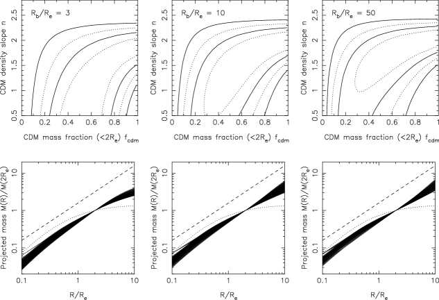
Figure 1: The structure of lens galaxies. All calculations assume a single star formation redshift (Model 1), but there is little change if we allow for a range of star formation redshifts (Model 2). Top: Constraints on the shape of the mass profile, which is set by the CDM mass fraction inside 2 effective radii ($f_{cdm}$), and the inner logarithmic slope of the CDM halo ($n$, with density $\rho\propto r^{-n}$). The halo is modeled with a cuspy profile (Muñoz et al. 2001), which breaks to an outer logarithmic slope of $3$ at a characteristic radius $R_{b}$. We show constraints for models with $R_{b}/R_{e}=3$, $10$ and $50$, where $R_{e}$ is the optical effective radius. Solid contours represent $\Delta\chi^{2}=2.30$ and $6.17$, the 68% and 95% confidence levels for two parameters. Dotted lines represent $\Delta\chi^{2}=1$ and $4$, the 68% and 95% confidence levels for one parameter. The errors have been rescaled so that the best-fit model has $\chi^{2}=N_{DOF}$. Bottom: The mass profiles of models favored at 68% confidence. Solid lines are the projected masses inside $R/R_{e}$. Profiles are normalized to a fixed projected mass at $R=2R_{e}$. For comparison we show the de Vaucouleurs profile (dotted line), and an offset isothermal profile (dashed line). While the allowed models exhibit a wide range of dark matter abundances and break radii, they all have total mass profiles which are approximately isothermal over the radial range spanned by the lensed images.

We begin by updating the RKK analysis of galaxy structure, taking into account the effects of galaxy evolution. To facilitate comparisons with the RKK results, we will derive our structural constraints using Model 1, which postulates a single star formation redshift. We assume the linear evolution model, but replacing this with the detailed evolutionary tracks has little quantitative effect. In Fig. 1 we plot constraints on the dark matter abundance $f_{cdm}$ and inner power-law slope $n$ by simultaneously optimizing the other parameters – $x$, $d\log(M/L)_{B}/dz$ and the normalization ($\gamma_{0}$ for the FP, $\Upsilon_{*}$ for the homology formalism). Solid lines are the 68% ($\Delta\chi^{2}<2.30$) and 95% ($\Delta\chi^{2}<6.17$) confidence limits in two dimensions; dotted lines are the 68% ($\Delta\chi^{2}<1$) and 95% ($\Delta\chi^{2}<4$) confidence limits in one dimension. These and all subsequent values of $\Delta\chi^{2}$ follow the setting of the scale factor $\delta_{scl}$ such that the best-fit model has $\chi^{2}=N_{DOF}$. Constraints are shown for three different values of the CDM break radius, $R_{b}/R_{e}=3$, $10$ and $50$. Smaller values of $R_{b}/R_{e}$ mean that the steep outer slope has a more prominent effect on the radial scales probed by the lens sample ($0.2<R/R_{e}<7$; see RKK). To compensate, the inner slope $n$ must become shallower as $R_{b}/R_{e}$ is decreased. The best-fit models have $\chi^{2}=44.1$, $43.8$ and $44.0$ for $R_{b}/R_{e}=3$, $10$ and $50$, respectively, corresponding to an rms scatter of $0.16$ in $\log(M/L)$. Based on our estimated uncertainties, this implies an intrinsic scatter of $\sim 30\%$. Note that a $\chi^{2}$ of $44$ for $N_{DOF}=17$ is a very poor fit, suggesting that structural homology and a single star formation redshift do not provide a good description of the lens data (see also vvF). This is also the case for the standard FP, whose intrinsic scatter is larger than can be explained by measurement errors alone (e.g., Jorgensen et al. 1996).

Our nearly identical values of $\chi^{2}$ for the different break radii indicate that our model is over-parameterized. For simplicity we will set $R_{b}/R_{e}=50$ for all subsequent calculations, and therefore treat the dark matter halo as a power law. Note, however, that this limit is not identical to the power-law surface mass $M(R)\propto R^{3-n}$ which RKK used to describe the halo. Specifically, the RKK model does not have a consistent three-dimensional projection for $n\leq 1$. As $n\rightarrow 1$ the two models are quantitatively different, with the RKK power law approaching a mass sheet ($\Sigma={\rm constant}$), and the cuspy model approaching a logarithmic surface density distribution ($\Sigma\propto\ln R$). Hence, for a given point ($f_{cdm}$ and $n\simeq 1$) in the parameter plane describing our new model, the projected mass profile is slightly steeper than the same point in the RKK model plane.

Despite our inability to separate the effects of the inner power-law slope, break radius and CDM mass fraction, all acceptable models are very close to isothermal on the scale of several effective radii. We plot the mass profiles in Fig. 1. Our profile constraints agree with those of RKK, who assumed a fixed evolution model corresponding to a star formation redshift of $z_{f}=3$. By including luminosity evolution as a free parameter, however, we allow for a slightly broader range of mass profiles. In the limit of a nearly scale-free mass model ($\Upsilon_{*}\rightarrow 0$, $f_{cdm}\rightarrow 1$, $R_{b}/R_{e}\gg 1$), our constraint on the logarithmic density slope is $n=2.06\pm 0.17$, compared to the RKK limit of $n=2.07\pm 0.13$. Each constraint is at 68% confidence, or $\Delta\chi^{2}<1$. We still detect dark matter to very high significance, as a model in which mass traces light is rejected at $\Delta\chi^{2}=9.2$ (compared to $\Delta\chi^{2}=10.7$ in RKK). In summary, uncertainties in the luminosity evolution do not affect our conclusions that early-type galaxies are nearly isothermal on the scale of a few effective radii, and that a small but non-zero fraction of dark matter ($f_{cdm}>0.08$, 95% C.L.) is required in this regime, independent of the stellar mass-to-light ratio.

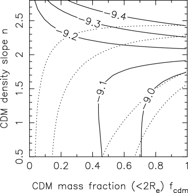
Figure 2: The recovered local FP intercept $\gamma_{0}$ as a function of mass profile, for $h=0.65$. We assume isotropic orbits ($\beta_{iso}=0$) and a cuspy dark matter halo with $R_{b}/R_{e}=50$. Velocity dispersions are estimated in an aperture with radius $R_{e}/8$. The FP slopes are fixed at $\alpha=1.25$ and $\beta=0.325$, corresponding to $x=0.3$. Solid lines are contours of best-fit $\gamma_{0}$. Dotted lines are the 68% and 95% confidence limits on the model (in two dimensions). These limits are slightly different than those shown in Fig. 1 because we have fixed the value of $x$. We find that the local FP intercept $\gamma_{0}$ varies slowly over our parameter space, and must therefore be measured to a precision of $\ll 0.1$ to improve the model constraints. Bender et al. (1998) measures $\gamma_{0}\sim-9.0$ for $\alpha=1.25$ and $\beta=0.32$.

The zero-point of the FP depends on some combination of the radial mass profile, mass-to-light ratio, orbital anisotropy and spectroscopic aperture, as these factors determine the dynamical constant $c_{M}$ (see eq. 7 and 8). If the local zero-point $\gamma_{0}$ has been accurately measured for a given set of slopes $\alpha$ and $\beta$, then the FP formalism adds information that is not included in the homology formalism, and could therefore improve our model constraints. We refit the intercept in our analysis because there is no accurate, independent measurement of $\gamma_{0}$ specifically for low-density environments. However, we can estimate the precision to which $\gamma_{0}$ must be measured in order to affect constraints on our structure/evolution model. In Fig. 2 we show the best-fit value of $\gamma_{0}$ as a function of mass profile. For demonstration purposes we assume FP slopes corresponding to $x=0.3$ ($\alpha=1.25$ and $\beta=0.325$), and calculate velocity dispersions for isotropic orbits ($\beta_{iso}=0$) in an aperture with radius $R_{e}/8$. We find that $\gamma_{0}$ varies slowly over the parameter plane if the FP slopes are fixed. The values vary wildly if $x$ is simultaneously fit. The value of $\gamma_{0}$ must be measured to a precision of $\ll 0.1$ to improve the model constraints. We therefore find that the FP adds little useful information beyond that already contained in the AMR relations.

While we have assumed that early-type galaxies are homologous, constraints on the typical mass profile (Fig. 1) show the range over which individual galaxy profiles might reasonably scatter. Dynamical studies of individual lenses can directly address departures from homology, and are therefore a powerful complement to our statistical analysis. Velocity dispersions have been measured for seven of the lenses in our sample: Q2237+0305 (Foltz et al. 1992), MG1549+3047 (Lehar et al. 1996), PG1115+080 (Tonry 1998), HST14176+5226 (Ohyama et al. 2002; Gebhardt et al. 2003; Treu & Koopmans 2004), MG2016+112 (Koopmans & Treu 2002), 0047–281 (Koopmans & Treu 2003), and B1608+656 (Koopmans et al. 2003). Two of the galaxies are particularly interesting, as dynamical measurements would imply that they have mass profiles which deviate significantly from isothermal. PG1115+080 (Weymann et al. 1980) has a velocity dispersion which is higher than the isothermal prediction, indicating a steeper mass profile (Tonry 1998; Treu & Koopmans 2002b). In contrast, HST14176+5226 (Ratnatunga et al. 1995) has a velocity dispersion which is lower than the isothermal prediction (Ohyama et al. 2002; Gebhardt et al. 2003; Treu & Koopmans 2004), indicating a shallower mass profile. Based on the existence of such structural outliers, it has been argued that estimated velocity dispersions are insufficient for evolution studies with gravitational lens samples. We now show that this will not be a significant concern for our new evolution constraints (§4.2).

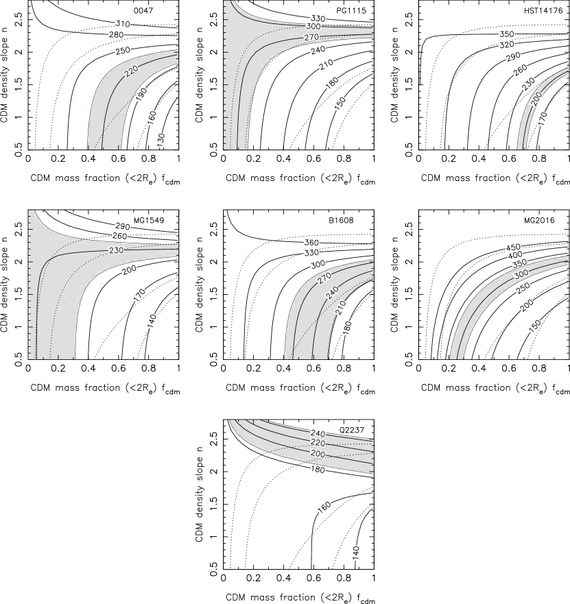
Figure 3: Velocity dispersions for lens galaxies. Solid lines are contours of constant velocity dispersion, estimated in circular apertures with area equal to that of the respective apertures in which they were observed. Dotted lines are the two-dimensional model constraints for $R_{b}/R_{e}=50$, shown in Fig. 1. The shaded areas are the measured velocity dispersions (68% C.L.). As previously noted, the dynamics of two galaxies may require profiles which are significantly different than isothermal. PG1115+080 is steeper, while HST14176+5226 is shallower. Substituting the higher Ohyama et al. (2002) or Treu & Koopmans (2004) velocity dispersion for the Gebhardt et al. (2003) value would bring HST14176+5226 into better agreement with our statistical results.

We wish to determine the degree to which dynamical measurements of lens galaxies are compatible with the range of mass profiles allowed by our FP/homology analysis. First, at each point in $(f_{cdm}-n)$ space, we set the profile normalization of the lens according to its AMR relation. We then estimate the velocity dispersion and compare it to the measured value. For our dynamical estimates we use a circular aperture with an area equal to that of the aperture in which the velocity dispersion has been measured, and assume isotropic orbits ($\beta_{iso}=0$). We expect our comparisons to be accurate at the level of $\sim 15\,{\rm km\,s^{-1}}$. For each lens, we plot in Fig. 3 contours of constant $\sigma$, along with our global profile constraints. We see that five of the seven lenses are nearly isothermal, and are consistent with our 68% confidence limits on the mean mass profile. Note that while our constraints on the individual mass profiles are qualitatively similar to those derived in the literature, there are small systematic disparities due to the use of differing structural parameters (effective radius, image separation, or environmental corrections). We confirm that the dynamical measurements of two galaxies require profiles that are formally inconsistent with isothermal. However, the comparison ignores systematic uncertainties in the dynamical model due to the derivation of velocity dispersions from Gaussian profiles and the ellipticities of the galaxies, each of which will reduce the significance of these deviations (see Kochanek, Schneider & Wambsganss 2004 for additional discussion). For PG1115+080, Tonry (1998) measures $\sigma=281\pm 25\,{\rm km\,s^{-1}}$ in a $1\farcs 0$ squared aperture. We find that this galaxy must have a profile which is significantly steeper than isothermal: $\rho\propto r^{-2.4}$, similar to the value favored by Treu & Koopmans (2002b). For HST14176+5226, Gebhardt et al. (2003) measure $\sigma=202\pm 9\,{\rm km\,s^{-1}}$ in a similar aperture, which is marginally inconsistent with a previous measurement of $\sigma=230\pm 14\,{\rm km\,s^{-1}}$ by Ohyama et al. (2002) and a similar measurement by Treu & Koopmans (2004). We plot the Gebhardt et al. (2003) value because it implies the greatest departure from the mean model. As expected, we find that HST14176+5226 requires a profile that is shallower than isothermal, with $\rho\propto r^{-1.7}$, and a rather high dark matter fraction ($f_{cdm}>0.6$). The discrepancy persists if we substitute the Ohyama et al. (2002) or Treu & Koopmans (2004) measurements, though at a reduced significance. While both PG1115+080 and HST14176+5226 appear to have mass profiles which are different than isothermal, Fig. 3 shows that the constraints on their profiles are consistent with our 95% confidence limit on the lens galaxy population – though only marginally consistent with our 68% confidence range. However, if the width of our statistical constraints reflects intrinsic scatter about the mean homology relation, then we might expect $\sim 1/3$ of lenses to be outliers at the level of PG1115+080 or HST14176+5226. This fraction is consistent with the present dynamical sample.

Consequently, our profile constraints are a sufficient proxy for measured velocity dispersions in gravitational lens galaxies. By simultaneously considering structure and evolution, we will derive limits on the evolution rate and mean star formation redshift which account for the allowed range over which galaxies may depart from a strict homology.

4.2 Focus on Luminosity Evolution

We now turn to luminosity evolution. Because of the large degeneracy between the CDM slope $n$ and abundance $f_{cdm}$, we will further simplify the total mass model to the scale-free limit ($\Upsilon_{*}\rightarrow 0$, $f_{cdm}\rightarrow 1$, $R_{b}/R_{e}\gg 1$). Note that this simplification does not have any effect on the evolution constraints versus the full mass model, but it does make it easier to display the results, particularly with regard to the interplay between mass concentration and evolution.

4.2.1 Model 1: Single Star Formation Redshift

We begin by analyzing Model 1, which postulates that lens galaxies were formed at a common epoch, and therefore follow a common evolutionary track as a function of redshift. This model is intended to describe the mean properties of the galaxy sample, and provide a standard for comparing results obtained by different groups. We reiterate, however, that this model does not provide a statistically good fit to the data. As we show in §4.2.2, including a range of star formation redshifts leads to a vastly improved model of the lens sample (see also vvF).

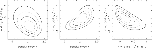
Figure 4: Constraints on the structure and evolution rate in Model 1. Plotted are pairwise constraints on the linear evolution rate $d\log(M/L)_{B}/dz$, mass-to-light ratio index $x$, and logarithmic density slope $n$ for a scale-free total mass distribution. Contours are drawn as in Fig. 1.

In Fig. 4 we plot pairwise constraints on the evolution rate $d\log(M/L)_{B}/dz$, mass-to-light ratio index $x$, and logarithmic density slope $n$, which now describes the total mass distribution. As we can see from Fig. 4, the parameters in our model are correlated. The anti-correlation between $x$ and $d\log(M/L)_{B}/dz$ is easiest to explain, as these two quantities enter the model as a product: $\log M(R)\propto(1+x)[\log L(z)+d\log(M/L)_{B}/dz\ z]$ (see eq. 12). This effect widens the favored range of $x$, compared to the constraints derived by RKK for a fixed $z_{f}=3$ evolution model. Specifically, we find $x=0.18^{+0.24}_{-0.18}$, while the RKK value is $x=0.14^{+0.16}_{-0.12}$ (both 68% C.L.). The source of the other correlations is not clear, though they may be related to the increasing mass scale of the lens sample with redshift (R03).

Optimizing over all structural parameters, we measure an evolution rate of $d\log(M/L)_{B}/dz=-0.50\pm 0.19$ at 68% confidence. The 95% confidence range is $-0.86<d\log(M/L)_{B}/dz<-0.10$. These constraints are identical for the full mass model and the scale-free limit, and are not significantly altered by setting $x$ to reflect locally measured FP slopes. Our results are consistent with the findings of R03, who measured $d\log(M/L)_{B}/dz=-0.54\pm 0.09$ (68% C.L.) from a sample of 28 lens galaxies under the assumption of isothermal mass profiles. Simultaneously optimizing the galaxy structure does weaken constraints on the evolution rate, but not to the point that they are uninteresting. The conclusion that lenses favor a slow evolution rate is unchanged.

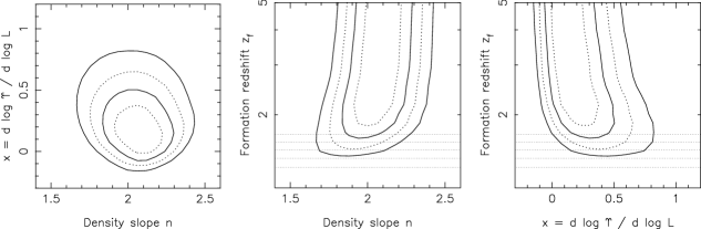
Figure 5: Constraints on the structure and mean star formation redshift $\langle z_{f}\rangle$ in Model 1. The panels are analogous to those in Fig. 4. Horizontal dotted lines mark $\langle z_{f}\rangle=1.3$, $1.4...1.7$. The lens sample favors old stellar populations, with $\langle z_{f}\rangle>1.5$ at 95% confidence.

We next consider bounds on the mean star formation redshift by using evolution tracks derived from the BC96 population synthesis models. Pairwise constraints are plotted in Fig. 5. The constraint on the mass-to-light ratio index ($x=0.14^{+0.22}_{-0.16}$, 68% C.L.) is somewhat tighter than that derived using the linear evolution rate. The small difference is due to the fact that the real tracks do not map into the linear tracks for later formation redshifts; e.g., there is no real track which is well approximated by a linear model for $z_{f}\lesssim 1.5$.

The best-fit model has a mean star formation redshift of $\langle z_{f}\rangle\simeq 2.2$, and the data are consistent with stellar ages as old as the universe itself. Coming from the other side, the constraints are far more restrictive: $\langle z_{f}\rangle>1.8$ at 68% confidence, and $\langle z_{f}\rangle>1.5$ at 95% confidence. Note that these results are not sensitive to our photometric conversion technique (§3.1). We find quantitatively similar bounds if the luminosities are derived from a $z_{f}=1.5$ spectrum, or from the spectra which best fit the colors of individual lenses. Excluding the four systems with estimated source redshifts slightly weakens the 95% confidence limit to $\langle z_{f}\rangle>1.4$.

The above evolution constraints are remarkable, considering that we have assumed no specific shape for the mass profile of lens galaxies. While we do assume that early-type galaxies comprise a regular population, the range of permitted profiles crudely approximates the degree of scatter allowed by the AMR relations. We can therefore account for possible departures from homology, without directly measuring individual velocity dispersions. Based on this simultaneous analysis of structure and evolution, we conclude that, on average, early-type galaxies in low-density environments have rather old stellar populations ($\langle z_{f}\rangle\simeq 2$), similar in age to their cluster counterparts.

4.2.2 Model 2: Range of Star Formation Redshifts

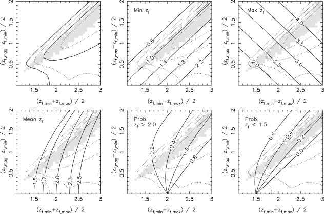
Figure 6: Top left: Constraints on the detailed star formation history of lens galaxies (Model 2). Stars form over an interval spanning $z_{f,min}$ to $z_{f,max}$, with uniform probability density in $\log z_{f}$. Confidence limits are plotted using solid and dotted contours as before, and are calculated from likelihood differences. We have optimized over all other model parameters. Significant scatter in $z_{f}$ is favored, and the single-$z_{f}$ scenario is excluded. Models which match the statistical properties of the actual lens sample are shaded in each panel. For these models, the lens data are consistent with the likelihood distribution determined from simulated data sets. The remaining panels show contours illustrating the distribution of star formation redshifts. Here our previous constraints are shown as dotted contours. Top center: Minimum $z_{f}$. Top right: Maximum $z_{f}$. Bottom left: Mean $z_{f}$. Bottom center: Fraction of galaxies forming at $z_{f}>2.0$. Bottom right: Fraction of galaxies forming at $z_{f}<1.5$.

We now turn to Model 2, which allows galaxies to form over a range of redshifts: $dP/d\log z_{f}={\rm constant}$ between $z_{f,min}$ and $z_{f,max}$. (Substituting a model in which the probability density of star formation is uniform over $z_{f}$, rather than $\log z_{f}$, has little effect on any of our primary results.) In Fig. 6 we plot constraints on the star formation model, optimizing over the global mass profile and mass-to-light ratio parameters. We have re-mapped the parameter space in terms of $(z_{f,min}+z_{f,max})/2$ and $(z_{f,max}-z_{f,min})/2$, as this better illustrates the physical meaning of the constraints. In the main panel (upper left), solid lines are the 68% ($\Delta\ln{\cal L}=-1.15$) and 95% ($\Delta\ln{\cal L}=-3.09$) confidence limits in two dimensions; dotted lines are the 68% ($\Delta\ln{\cal L}=-0.5$) and 95% ($\Delta\ln{\cal L}=-2.0$) confidence limits in one dimension. In subsequent panels of Fig. 6 we overlay contours to better describe the distribution of star formation redshifts in the model. Specifically, we plot the minimum, maximum and mean formation redshifts, as well as the fraction of stars forming earlier than $z_{f}=2.0$ and later than $z_{f}=1.5$.

The lens sample favors models with significant scatter in star formation redshift: $z_{f,max}-z_{f,min}>0.4$ at 95% confidence and $z_{f,max}-z_{f,min}>1.7$ at 68% confidence, each based on one-dimensional likelihood differences. The required scatter in $z_{f}$ increases with mean star formation redshift. This can be understood by noting that luminosity evolution depends much more sensitivity on $z_{f}$ when $z_{f}$ is small. At higher mean formation redshifts, a broader redshift range is required to produce the same luminosity scatter for galaxies at $z<1$. The nearly linear nature of the degeneracy – $(z_{f,max}-z_{f,min})/2\propto(z_{f,min}+z_{f,max})/2$ – indicates that the analysis is most sensitive to $z_{f,min}$, which is consistent with the rapid variation of evolutionary tracks for late formation redshifts. For the lens sample, $z_{f,min}$ cannot be much smaller than 1. Undoubtedly the high redshift ($z>0.5$) lens galaxies will dominate this constraint, as they are most sensitive to $z_{f}$. In contrast, models with much later star formation could be allowed if only low redshift lenses were considered. We note that the distribution of star formation redshifts can vary significantly among acceptable models of the lens sample. For example, the most favored models ($\Delta{\cal L}<-1.15$) allow anywhere from $0$ to $40\%$ of galaxies to form at $z_{f}<1.5$ (Fig. 6). We therefore conclude that low-redshift star is an important component of our model. However, in all of our acceptable models the mean star formation redshift is relatively high ($\langle z_{f}\rangle>1.5$).

It is interesting to note that allowing a range of star formation redshifts leads to a relatively modest improvement versus a single-$z_{f}$ scenario, at least from a maximum likelihood perspective. For example, we find that the best-fit single-$z_{f}$ model ($z_{f,min}=z_{f,max}\sim 2.2$) is at only $\Delta\ln{\cal L}=-2.1$ with respect to the best overall model. There is, however, a large improvement in terms of finding models which provide a good statistical description of the data. As the spread in $z_{f}$ is increased from zero, the likelihood describing the data ($\ln{\cal L}$) increases slowly, while the mean likelihood of data sets drawn from the Monte Carlo ($\langle\ln{\cal L}_{sim}\rangle$) decreases due to the fact that the model is inherently more diffuse. This leads to a rapid improvement in matching the statistical properties of the lens sample to that of the models. For example, the best-fit single-$z_{f}$ model has a likelihood which is lower than its corresponding $\langle\ln{\cal L}_{sim}\rangle$ by $|\Delta\ln{\cal L}|\sim 12$ (this is nearly equal to $(\chi^{2}-N_{DOF})/2$, as expected), and well outside the range described by $\ln{\cal L}_{sim}^{STD}$. Models with a single star formation redshift are thus clearly inconsistent with the statistical properties of the data. However, by $z_{f,max}-z_{f,min}\sim 1$ we find models for which $|\ln{\cal L}-\langle\ln{\cal L}_{sim}\rangle|\leq\ln{\cal L}_{sim}^{STD}$. Such models meet the necessary condition for statistical compatibility, in the sense that the real lens sample may actually be drawn from them. This regime is marked by the shaded area in each panel of Fig. 6.

In conclusion, models in which early-type field galaxies form homologously over a range of redshifts offer a vastly improved representation of the actual lens sample. Allowing some fraction of galaxies to form at low redshift is an important component of these models, though the mean star formation redshift is still relatively high. The best-fit models meet the necessary condition for statistical consistency with the lens sample, based on the interpretation of likelihoods. As noted in §3.1, altering the assumed luminosity errors does not change this conclusion.

5 Are Lensing Analyses Consistent?

5.1 Statistical Results

The luminosity evolution of gravitational lens galaxies has recently been explored by van de Ven et al. (2003), who use the FP to derive an evolution rate of $d\log(M/L)_{B}/dz=-0.62\pm 0.13$ from a sample of 26 lenses. This is slightly faster than the findings of either R03 ($-0.54\pm 0.09$) or this paper ($-0.50\pm 0.19$ for Model 1), even though the lens samples and photometry are nearly the same. Furthermore, vvF claim that rather late mean star formation redshifts are permitted ($\langle z_{f}\rangle=1.8^{+1.4}_{-0.5}$, 68% C.L.), while much of this range is excluded by R03 ($\langle z_{f}\rangle>1.8$, 95% C.L.) and the combined structure/evolution analysis of §4.2.1 ($\langle z_{f}\rangle>1.5$, 95% C.L.). While the results of RKK and vvF are technically consistent, it is instructive to discuss three factors which account for the small differences: data weighting, stellar evolution models, and sample selection.

First, differences in data weighting account for most of the systematic disparity in evolution rates. We set a fixed uncertainty for all galaxy luminosities, ensuring that each lens has a similar relative contribution to the fit. In contrast, vvF use uncertainties which they derive from their photometric conversion. Based on their quoted errors on the surface brightness, some galaxies are far more important to the fit than other galaxies. Data weighting has a surprisingly large impact on the derived evolution rate. vvF already demonstrate this by testing an error term (to account for scatter) which is added in quadrature with other errors. This has the effect of weighting the galaxies more uniformly, and slows the evolution rate from $d\log(M/L)_{B}/dz=-0.62\pm 0.13$ to $-0.56\pm 0.12$. We have confirmed these results by reanalyzing the data tabulated in vvF. Furthermore, we find that the vvF data yield an even slower evolution rate of $d\log(M/L)_{B}/dz=-0.46\pm 0.12$ (very similar to our value) if we impose uniform weighting. The choice of weighting is clearly important for constraining the evolution model, and the vvF method is not unreasonable. However, we believe that our scheme provides a more realistic description of the global properties of the lens galaxy population, since uncertainties in Model 1 are certain to be dominated by intrinsic scatter in the mass profile and formation redshift, rather than by measurement errors. Galaxies should not be segregated based on nominal photometric errors if those errors are much too small to account for the observed scatter in the FP. Moreover, weighting galaxies by their photometric errors can introduce a Malmquist bias, which we may be seeing in the vvF analysis. Relatively brighter galaxies are expected to have better photometry, giving them greater statistical weight. Since brighter galaxies at high redshift will also imply a greater degree of luminosity evolution, the mean evolution rate will tend to be biased toward faster values. Nearby lens galaxies, which are bright but have little ability to distinguish between star formation models, would also be more strongly weighted than the distant galaxies which are vital for determining stellar age through luminosity evolution.

Second, the constraints on stellar age are affected by models of the evolution tracks $e(z)$ as a function of star formation redshift. We use the tracks derived from the BC96 stellar synthesis code. In contrast, vvF use an approximation to the Worthey (1994) simulation results: $\log(M/L)_{B}\propto\kappa\log(t-t_{f})$, where $t-t_{f}$ is the stellar age and $\kappa\simeq 0.93$. The models agree very well for $z_{f}\gtrsim 2$, but the BC96 model evolves more rapidly than the vvF fitting function for $z_{f}\leq 1.5$. As a result, later star formation redshifts are more strongly disfavored with the BC96 model, which tightens our lower bound on $\langle z_{f}\rangle$. We tested this hypothesis by reanalyzing the vvF data (with their quoted uncertainties). For example, while vvF find that their $z_{f}=1.3$ track is marginally consistent with their data, the corresponding BC96 track is unambiguously rejected at $\Delta\chi^{2}=12$. We believe that the BC96 model facilitates more accurate constraints on the mean star formation redshift, as it offers a more detailed treatment of young stellar populations than the vvF approximation.

Third, differences in sample selection have a small systematic effect on the evolution results. Systems without measured source redshifts are rejected by vvF, but are included in our analysis (with an estimate of $z_{s}=2.0\pm 1.0$). Two of these systems – MG1131+0456 (Hewitt et al. 1988) and B1938+666 (Patnaik et al. 1992) – are particularly interesting. Each is at high redshift ($z_{d}=0.84$ and $0.88$, respectively) and exhibits a larger than average mass-to-light ratio (especially MG1131+0456). Hence, they force the model to slightly slower evolution rates. While excluding such systems alters constraints on the mean star formation redshift at the level of only $\sim 0.1$ (see §4.2), there is no reason that these lenses should be rejected just because they are outliers. In all other respects, they look like typical elliptical galaxies (Tonry & Kochanek 2000). One may argue, however, that our choice for the estimated source redshift biases the result. We note that the implied mass-to-light ratios of these galaxies can be reduced if the sources are at a much higher redshift ($z_{s}\gtrsim 4$). Based on the optical properties of the sources, this is indeed a reasonable scenario. However, we find that these systems have an equally important role in the fit even if we substitute “measured” values of $z_{s}=4.0$ for our estimated values of $z_{s}=2.0\pm 1.0$ – while the absolute deviation from the global model is reduced, this is almost completely compensated by the reduced fit tolerance for systems with a measured $z_{s}$. Therefore, the inclusion of these systems in our analysis is strongly justified, and their effects on the fit are real.

Finally, it is interesting to note that R03 and vvF have no systematic differences in rest frame magnitudes, despite using alternate techniques for photometric conversion. However, vvF appear to have more scatter in their data points, and we trace this to the photometry. Larger scatter slightly broadens the vvF confidence regions compared to our own, and therefore leads to a somewhat weaker rejection of late formation redshifts.

5.2 Individual Lenses

Several studies have focussed on the structure and evolution of individual lens galaxies (Treu et al. 2002a,b; Koopmans & Treu 2003; Koopmans et al. 2003; Gebhardt et al. 2003; Treu & Koopmans 2004). While these analyses have the benefit of using measured velocity dispersions in the fundamental plane relation, there are also two significant drawbacks. First, to determine the evolution implied by a single galaxy or a small number of galaxies, one must make an explicit comparison against a local FP intercept measured from other samples. This often means using the intercept for ellipticals in the Coma cluster to evaluate the evolution of field galaxies, even though these populations should not, in general, have identical intercepts at $z=0$. Second, such studies may be susceptible to a Malmquist bias, which presumably makes it easier to measure velocity dispersions in more luminous, higher surface brightness galaxies with younger stellar populations. In this case, a sample of lenses with measured velocity dispersions, especially at higher redshift, would be biased toward faster evolution rates. Such effects may already be evident in the current dynamical sample.

The Lens Structure and Dynamics survey (LSD; Koopmans & Treu 2002, 2003; Treu & Koopmans 2002a; Koopmans et al. 2003; Treu & Koopmans 2004) has measured the velocity dispersions of several gravitational lenses, which are combined with HST photometry to constrain structure and evolution. Five of these lenses appear in our sample: MG2016+112 (Lawrence et al. 1984), 0047–281 (Warren et al. 1996), B1608+656 (Myers et al. 1995), HST14176+5226 (Ratnatunga et al. 1995), and PG1115+080 (Weymann et al. 1980). As we discussed in §4.1, our statistical constraints on the galaxy mass profile are largely consistent with those derived through dynamical measurements and modeling. Note, however, that Treu & Koopmans (2004) now favor a mean logarithmic slope which is significantly shallower and marginally inconsistent with isothermal, based on a combined analysis of six lens galaxies. Two of these galaxies do not currently appear in our sample, and help weight the LSD analysis toward shallower profiles.

The LSD sample also favors faster evolution rates and younger stellar populations than our results indicate. This may be due in part to a luminosity-related selection bias, or at least small number statistics. For example, our evolution results for MG2016+112 and 0047–281, based on a fixed local FP intercept, agree well with those measured in the LSD survey – but each lens scatters on the “young” side of our evolutionary trend-lines. Moreover, the LSD survey has observed B1608+656, whose spectral properties suggest that the galaxy has undergone significant star formation triggered by an ongoing merger (Koopmans et al. 2003). Using dust corrections based on observed color gradients, they derive a luminosity which is much larger than that of passively-evolving galaxies, and a luminosity evolution which is much faster than our estimate for the overall sample. Based on an analysis of their lens sample, Treu & Koopmans (2004) find an evolution rate of $d\log(M/L)_{B}/dz=-0.72\pm 0.10$, which is systematically faster but still broadly consistent with the evolution rate we derive by optimizing over the mass profile.

Departures from homology can also have interesting effects on the derived evolution rates. If we compare the implied FP intercept with a fixed local value, then a larger velocity dispersion yields a slower evolution rate, and vice versa. PG1115+080, whose measured velocity dispersion is much higher than the isothermal prediction (Tonry 1998; Treu & Koopmans 2002b), must undergo virtually no luminosity evolution to $z=0.31$ if it is to fall on the local FP. Alternatively, if the galaxy evolves at a standard evolution rate, its structure cannot be consistent with the rest of the early-type galaxy population. HST14176+5226, in contrast, yields a significantly faster evolution rate if the isothermal velocity dispersion estimate is replaced with one of its measured values. Unless the quoted error bars on the velocity dispersions have been underestimated, the findings of Gebhardt et al. (2003), Treu & Koopmans (2004) and others suggest that early-type galaxies exhibit significant structural diversity. Such deviations from homology warn against using small numbers of lenses to constrain an evolution model meant to describe the galaxy population as a whole.

6 Summary and Discussion

Evolution studies of early-type galaxies based on gravitational lens samples (Kochanek et al. 2000; R03; vvF) have often been criticized for using estimated, rather than measured, velocity dispersions, because a mass model is required to convert the accurately measured projected mass into a dynamical estimate. The primary concern has been that the preferred mass model for lenses, an isothermal model with a flat rotation curve, could be incorrect. The secondary concern is that early-type galaxies may not be well characterized by any single mass distribution that is homologous to the luminosity distribution. By simultaneously modeling both the structure and evolution of lens galaxies, our present analysis helps address these concerns. Specifically, we determine the best-fit mass profile for lens galaxies (as well as the range over which individual lenses might scatter), and account for these effects on the mean evolution model. Our technique builds on the homologous two-component mass models of RKK, which were constrained using the ensemble of aperture mass-radius relations derived from lensed image geometries. The homology formalism is virtually identical to the fundamental plane, with the AMR relations substituting for measured velocity dispersions. In essence, this allows us to trace luminosity evolution with the FP, while directly using the quantity (aperture mass) that strong lensing naturally constrains.

We first updated constraints on the structure of early-type galaxies, assuming that lenses are characterized by a single star formation redshift. We find that uncertainty in the evolution model has little effect on our structural results. The FP strongly favors nearly isothermal ($n=2$) mass profiles on scales of a few effective radii, with a mean density slope of $n=2.06\pm 0.17$ (68% C.L.). These statistical constraints are consistent with the isothermal paradigm favored by modeling (Kochanek 1995; Cohn et al. 2001; Muñoz et al. 2001; Rusin et al. 2002; Winn et al. 2003) and dynamical (Treu & Koopmans 2002a, 2002b; Koopmans & Treu 2003; Koopmans et al. 2003) studies of individual lens galaxies, the dynamics of local ellipticals (e.g., Rix et al. 1997; Romanowsky & Kochanek 2001; Gerhard et al. 2001), and their X-ray halos (e.g., Fabbiano 1989; Matsushita et al. 1998; Loewenstein & White 1999). Note, however, that Treu & Koopmans (2004) favor models with systematically shallower profiles, while Romanowsky et al. (2003) favor significantly more concentrated models. Our analysis indicates that a small but non-zero fraction ($f_{cdm}>0.08$, 95% C.L.) of the mass projected inside two effective radii must be in the form of an extended dark matter halo, independent of any assumed stellar mass-to-light ratio. We also constrain the increase in the total mass-to-light ratio with galaxy luminosity ($\Upsilon_{*}\propto L^{x}$) : $x=0.18^{+0.24}_{-0.18}$ for the linear evolution model, and $x=0.14^{+0.22}_{-0.16}$ for the detailed BC96 evolution tracks (both 68% C.L.). These results are consistent with recent dynamical analyses of early-type galaxies (Gerhard et al. 2001; Bernardi et al. 2003; Borriello et al. 2003; Padmanabhan et al. 2004). Because the FP is closely related to the homology formalism, our constraint on $x$ can be considered the first constraint on the slopes of the lensing fundamental plane: $1.1<\alpha<2.0$ and $0.3<\beta<0.4$. These constraints are not yet very restrictive, but they are consistent with measurements of the local FP (e.g., Jorgensen et al. 1996; Pahre et al. 1998a; Bernardi et al. 2003).

Next we considered the luminosity evolution of lens galaxies, and find a small effect from the uncertainties in the mass model. We began by investigating a model in which all galaxies form at a common redshift (Model 1). The same assumption has been made in almost every analysis of early-type galaxies, and therefore provides a basis for comparing results. The lens sample favors a linear evolution rate of $d\log(M/L)_{B}/dz=-0.50\pm 0.19$ (68% C.L.). This constraint includes the spread in structural properties that are consistent with the AMR relations, and is therefore weaker than the value derived by R03 based on isothermal profiles, $d\log(M/L)_{B}/dz=-0.54\pm 0.09$ (68% C.L.). Assuming the standard cosmological parameters and a Salpeter IMF, we require a mean star formation redshift of $\langle z_{f}\rangle>1.8$ at 68% confidence, and $\langle z_{f}\rangle>1.5$ at 95% confidence, based on the BC96 spectral population models. These constraints are remarkable, considering that we make no assumption regarding the shape of the galaxy mass distribution or the slopes of the fundamental plane. Our only assumption is that these galaxies are structurally homologous, but even this is not restrictive: we obtain identical conclusions if the increase in mass-to-light ratio with luminosity is modeled as a systematic non-homology. We favor slightly older stellar populations in lens galaxies than van de Ven et al. (2003), who suggest that lenses could be consistent with mean star formation redshifts as late as $\langle z_{f}\rangle\sim 1.2$. We have traced these differences to data weighting, evolution models and sample selection. In conclusion, our single-$z_{f}$ analysis again indicates that, on average, early-type galaxies in low-density environments have old stellar populations – perhaps as old as their counterparts in rich clusters.

Model 1 does not provide a good fit to the data given the estimated statistical uncertainties, much as the scatter in the standard FP also exceeds measurement errors. This suggests that additional sources of complexity have not been properly taken into account. In particular, we can be confident that galaxies are neither perfectly homologous nor form at a common redshift. The scatter about our best fitting solution corresponds to a spread of approximately 30–35% in some combination of mass (deviations from homology) and luminosity (range of star formation epochs). For our overall constraints on the mean structure and the mean star formation redshift, we included these additional uncertainties in our error estimates.

We explored one source of this scatter using the seven lens systems in our sample with direct velocity dispersion measurements. For each system we can estimate the parameters of the mass model needed to reconcile the velocity dispersion with the aperture mass constraint. In general, all seven are consistent with our statistical results, given their mutual errors. This is just a rephrasing of the fact that our error estimates in Model 1 have correctly included the scatter created by deviations from homology or a spread in formation epochs. Four of the seven lenses have parameters and parameter degeneracies similar to our statistical models. PG1115+080 requires a steeper mass distribution, while HST14176+5226 requires a shallower mass distribution. However, systematic errors in measuring and modeling stellar velocity dispersions might significantly mitigate these discrepancies. Q2237+0305, the bulge of a nearby spiral galaxy (Huchra et al. 1985), should probably be described by a more complex mass model, but an isothermal profile can still describe its inner dynamics.

We also investigated a model which can directly account for the observed scatter in the homology relation by allowing a range of star formation redshifts. Specifically, we assumed that stars form between $z_{f,min}$ and $z_{f,max}$, with uniform probability density in $\log z_{f}$, and that the galaxies are structurally homologous at formation. By ignoring any intrinsic distribution of mass profiles, we expect to maximize the range of formation redshifts necessary to reproduce the observed scatter. Applying a likelihood analysis to the lenses, we find that a significant spread in formation redshift is favored: ($z_{f,max}-z_{f,min}>0.4$ at 95% confidence, and $z_{f,max}-z_{f,min}>1.7$ at 68% confidence), while the single-$z_{f}$ model is ruled out. Moreover, simulated data sets created from a subset of the acceptable models yield likelihoods similar to that of the real data. Allowing a range of formation redshifts therefore provides a vastly improved statistical description of the lens sample. The required scatter in $z_{f}$ increases almost linearly with the mean star formation redshift. This can be understood by noting that luminosity evolution depends much more sensitively on $z_{f}$ when $z_{f}$ is small. We find that the distribution of star formation redshifts can vary significantly among acceptable models of the lens sample. For example, the most favored models ($\Delta{\cal L}<-1.15$) allow anywhere from $0$ to $40\%$ of galaxies to form at $z_{f}<1.5$ (Fig. 6). We therefore conclude that the stars in early-type field galaxies form over a substantial range of redshifts, and that some fraction of these stars may have formed as recently as $z_{f}\sim 1$. Our analysis bolsters the findings of Treu et al. (2001, 2002), van de Ven et al. (2003), Koopmans et al. (2003), and van der Wel et al. (2004), who argue that late star formation in some fraction of field ellipticals is essential for explaining their evolutionary history. However, we depart from a few recent claims (Treu et al. 2001, 2002; Gebhardt et al. 2003) that the mean star formation redshift of field ellipticals may be as late as $z_{f}=1$. In all of our statistically acceptable models, the mean star formation redshift is relatively high ($\langle z_{f}\rangle>1.5$).

Understanding the star formation history of early-type field galaxies remains a work in progress. There is, however, growing consistency among results based on colors (Menanteau et al. 2001; vvF; Bell et al. 2004), spectral properties (Bernardi et al. 1998; Schade et al. 1999; Kuntschner et al. 2002; Treu et al. 2002) and the fundamental plane (Kochanek et al. 2000; van Dokkum et al. 2001; Treu et al. 2001, 2002; Rusin et al. 2003; van de Ven et al. 2003; van Dokkum & Ellis 2003; van der Wel et al. 2004; Treu & Koopmans 2004; this paper). Taken together, these analyses present a strong case that field ellipticals formed the bulk of their stars between $z_{f}=1.5$ and $2.0$, and are therefore not much younger than their counterparts in high-density environments. This largely disagrees with the predictions of semi-analytic CDM models (e.g., Baugh et al. 1996; Kauffmann 1996; Kauffman & Charlot 1998; Diaferio et al. 2001). Moreover, based on the internal scatter of the various samples, it appears that the stars in field ellipticals are likely to have formed over a range of redshifts, with some fraction of the stars forming as late as $z_{f}\sim 1$. The degree to which these galaxies experience late star formation is a subject of continuing debate, and several of the above results disagree on the details.

What is the source of these remaining discrepancies among analyses of early-type field galaxies? Sample selection is probably the best starting hypothesis. Each of the above evolution studies employs different criteria for selecting early-type galaxies. For example, Treu et al. (2001, 2002) use morphological/magnitude/color cuts, van Dokkum & Ellis (2003) use morphological/magnitude cuts, and Gebhardt et al. (2003) use the bulge fraction. The lens sample, by contrast, is selected on mass, with large velocity dispersion ellipticals dominating the lensing optical depth. The mass selection makes the gravitational lens sample unique, as it is the only one not to be affected by Malmquist biases related to luminosity, color, or other star formation signatures. However, lensing also selects more massive samples of ellipticals. Assuming an isothermal profile, the 22 lenses we analyzed have a mean velocity dispersion of $\sim 240\,{\rm km\,s^{-1}}$, about $10-25\%$ higher than any of the other samples listed above. The mean velocity dispersion of lens galaxies also increases with redshift, due to angular selection effects (R03). Because there is evidence to indicate that more massive early-type galaxies may be older (van der Wel et al. 2004), the higher mean velocity dispersion of the lens sample could partially account for its slower evolution rate. Additional work is clearly necessary to quantify the benefits and biases of the various samples.

Whatever the remaining uncertainties, the lens galaxies are an extraordinarily powerful probe of galactic structure and evolution. Using only 22 lenses, we can simultaneously constrain the mean mass profile of early-type galaxies, the dependence of the mass-to-light ratio on luminosity, and the rate of stellar evolution, with statistical and systematic uncertainties that are competitive with all other methods. The power of gravitational lenses is a result of the aperture mass-radius relations derived from the image geometries, but good photometry and measured redshifts are needed to make use of these constraints. Follow-up imaging and spectroscopy is therefore vital to expanding the current lens sample, which may soon enable significantly improved statistical analyses. Such future studies could investigate lenses as a function of color, velocity dispersion, environment or spectral properties. In addition, a sufficiently large sample of lenses could probe not only luminosity evolution, but structural evolution as well (e.g., Mao & Kochanek 1994; Rix et al. 1994; Ofek, Rix & Maoz 2003), thereby tracing the merger history in low-density environments. Detailed dynamical studies of individual lenses, such as those being carried out by the LSD survey, are also vital, as they can directly map the diversity of the lens galaxy population. Similar physical constraints can be obtained using time delay measurements in gravitational lenses, if we can safely assume that the Hubble constant is accurately measured. With a known Hubble constant, time delays measure the surface mass density near the lensed images (Kochanek 2002), which would break the model degeneracies for individual lenses in the same manner as a velocity dispersion measurement. Models for the time variability created by the microlensing of lensed images can also help break the degeneracy because the light curves can be used to determine the fraction of the surface mass density in the form of stars (Kochanek 2004; see also Schechter & Wambsganss 2002 for a discussion of statistical constraints based on flux ratio anomalies). Because of their unique properties, gravitational lenses will continue to contribute significantly to our knowledge of early-type galaxies, and provide a testing ground for galaxy formation theories.

References

- (1)
- (2) Baugh, C.M., Cole, S., & Frenk, C.S. 1996, MNRAS, 283, 1361
- (3)
- (4) Bell, E.F., Wolf, C., Meisenheimer, K., Rix, H.-W., Borch, A., Dye, S., Kleinheinrich, M., Wisotzki, L., & McIntosh, D.H. 2004, ApJ, 608, 752
- (5)
- (6) Bender, R., Saglia, R.P., Ziegler, B., Belloni, P., Greggio, L., Hopp, U., & Bruzual, G. 1998, ApJ, 493, 529
- (7)
- (8) Bernardi, M., Renzini, A., da Costa, L.N., Wegner, G., Alonso, M.V., Pellegrini, P.S., Rité, C., & Willmer, C.N.A. 1998, ApJL, 508, L143
- (9)
- (10) Bernardi, M., et al. 2003, AJ, 125, 1866
- (11)
- (12) Bertin, G., et al. 1994, A&A, 292, 381
- (13)
- (14) Bertin, G., Ciotti, L., & Del Principe, M. 2002, A&A, 386, 149
- (15)
- (16) Borriello, A., Salucci, P., & Danese, L. 2003, MNRAS, 341, 1109
- (17)
- (18) Bower, R.G., Lucey, J.R., & Ellis, R.S. 1992, MNRAS, 254, 601
- (19)
- (20) Bruzual, A.G., & Charlot, S. 1993, ApJ, 405, 538
- (21)
- (22) Caon, N., Capaccioli, M., & D’Onofrio, M. 1993, MNRAS, 265, 1013
- (23)
- (24) Ciotti, L., Lanzoni, B., & Renzini, A. 1996, MNRAS, 282, 1
- (25)
- (26) Cohn, J.D., Kochanek, C.S., McLeod, B.A., & Keeton, C.R. 2001, ApJ, 554, 1216
- (27)
- (28) Cole, S., Aragon-Salamanca, A., Frenk, C.S., Navarro, J.F., & Zepf, S.E. 1994, MNRAS, 271, 781
- (29)
- (30) Davis, M., Efstathiou, G., Frenk, C.S., & White, S.D.M. 1985, ApJ, 292, 371
- (31)
- (32) Diaferio, A., Kauffmann, G., Balogh, M.L., White, S.D.M., Schade, D., & Ellingson, E. 2001 MNRAS, 323, 999
- (33)
- (34) Djorgovski, S., & Davis, M. 1987, ApJ, 313, 59
- (35)
- (36) Dressler, A., Lynden-Bell, D., Burstein, D., Davies, R.L., Faber, S.M., Terlevich, R., & Wegner, G. 1987, ApJ, 313, 42
- (37)
- (38) Ellis, R.S., Smail, I., Dressler, A., Couch, W.J., Oemler, A., Jr., Butcher, H., & Sharples, R.M. 1997, ApJ, 483, 582
- (39)
- (40) Fabbiano, G. 1989, ARA&A, 27, 87
- (41)
- (42) Faber, S.M., Dressler, A., Davies, R.L., Burstein, D., & Lynden-Bell, D. 1987, in: Nearly normal galaxies, ed. S.M. Faber (New York: Springer), 175
- (43)
- (44) Ferreras, I., Charlot, S., & Silk, J. 1999, ApJ, 521, 81
- (45)
- (46) Foltz, C.B., Hewett, P.C., Webster, R.L., & Lewis, G.F. 1992, ApJL, 386, L43
- (47)
- (48) Gebhardt, K., et al. 2003, ApJ, 597, 239
- (49)
- (50) Gerhard, O., Kronawitter, A., Saglia, R.P., & Bender, R. 2001, AJ, 121, 1936
- (51)
- (52) Hernquist, L. 1990, ApJ, 356, 359
- (53)
- (54) Hewitt, J.N., Turner, E.L., Schneider, D.P., Burke, B.F., & Langston, G.I. 1988, Nature, 333, 537
- (55)
- (56) Holtzman, J.A., Burrows, C.J., Casertano, S., Hester, J.J., Trauger, J.T., Watson, A.M., & Worthey, G. 1995, PASP, 107, 1065
- (57)
- (58) Huchra, J., Gorenstein, M., Kent, S., Shapiro, I., Smith, G., Horine, E., & Perley, R. 1985, AJ, 90, 691
- (59)
- (60) Im, M., et al. 2002, ApJ, 571, 136
- (61)
- (62) Jorgensen, I., Franx, M., & Kjaergaard, P. 1996, MNRAS, 280, 167
- (63)
- (64) Jorgensen, I., Franx, M., Hjorth, J., & van Dokkum, P.G. 1999, MNRAS, 308, 833
- (65)
- (66) Kauffmann, G., White, S.D.M., & Guiderdoni, B. 1993, MNRAS, 264, 201
- (67)
- (68) Kauffmann, G. 1996, MNRAS, 281, 487
- (69)
- (70) Kauffmann, G., & Charlot, S. 1998, MNRAS, 294, 705
- (71)
- (72) Kauffmann, G., et al. 2003, MNRAS, 341, 33
- (73)
- (74) Keeton, C.R., Kochanek, C.S., & Falco, E.E. 1998, ApJ, 509, 561
- (75)
- (76) Keeton, C.R., Christlein, D., & Zabludoff, A.I. 2000, ApJ, 545, 129
- (77)
- (78) Kelson, D.D., van Dokkum, P.G., Franx, M., Illingworth, G.D., & Fabricant, D. 1997, ApJL, 478, L13
- (79)
- (80) Kelson, D.D., Illingworth, G.D., van Dokkum, P.G., & Franx, M. 2000, ApJ, 531, 184
- (81)
- (82) Kochanek, C.S. 1994, ApJ, 436, 56
- (83)
- (84) Kochanek, C.S. 1995, ApJ, 445, 559
- (85)
- (86) Kochanek, C.S., et al. 2000, ApJ, 543, 131
- (87)
- (88) Kochanek, C.S. 2002, ApJ, 578, 25
- (89)
- (90) Kochanek, C.S. 2004, ApJ, 605, 58
- (91)
- (92) Kochanek, C.S. Schneider, P., & Wambsganss, J. 2004, Gravitational Lensing: Strong, Weak & Micro, Proceedings of the 33rd Saas-Fee Advanced Course, G. Meylan, P. Jetzer & P. North, eds. (Berlin: Springer-Verlag)
- (93)
- (94) Koopmans, L.V.E., & Treu, T. 2002, ApJL, 568, L5
- (95)
- (96) Koopmans, L.V.E., & Treu, T. 2003, ApJ, 583, 606
- (97)
- (98) Koopmans, L.V.E., Treu, T., Fassnacht, C.D., Blandford, R.D., & Surpi, G. 2003, ApJ, 599, 70
- (99)
- (100) Kuntschner, H., Smith, R.J., Colless, M., Davies, R.L., Kaldare, R., & Vazdekis, A. 2002, MNRAS, 337, 172
- (101)
- (102) Lawrence, C.R., Schneider, D.P., Schmidet, M., Bennett, C.L., Hewitt, J.N., Burke, B.F., Turner, E.L., & Gunn, J.E. 1984, Sci, 223, 46
- (103)
- (104) Lehar, J., Cooke, A.J.; Lawrence, C.R., Silber, A.D., & Langston, G.I. 1996, AJ, 111, 1812
- (105)
- (106) Loewenstein, M., & White, R.E. 1999, ApJ, 518, 50
- (107)
- (108) Madgwick, D.S., et al. 2002, MNRAS, 333, 133
- (109)
- (110) Mao, S.D., & Kochanek, C.S. 1994, MNRAS, 268, 569
- (111)
- (112) Matsushita, K., Makishima, K., Ikebe, Y., Rokutanda, E., Yamasaki, N., & Ohashi, T. 1998, ApJL, 499, L13
- (113)
- (114) Menanteau, F., Abraham, R.G., & Ellis, R.S. 2001, MNRAS, 322, 1
- (115)
- (116) Merritt, D. 1985a, AJ, 90, 1027
- (117)
- (118) Merritt, D. 1985b, MNRAS, 214, 25
- (119)
- (120) Moore, B., Quinn, T., Governato, F., Stadel, J., & Lake, G. 1999, MNRAS, 310, 1147
- (121)
- (122) Myers, S.T., et al. 1995, ApJL, 447, L5
- (123)
- (124) Muñoz, J.A., Kochanek, C.S., & Keeton, C.R. 2001, ApJ, 558, 657
- (125)
- (126) Navarro, J.F., Frenk, C.S., & White, S.D.M. 1997, ApJ, 490, 493
- (127)
- (128) Ofek, E.O., Rix, H.-W., & Maoz, D. 2003, MNRAS, 343, 639
- (129)
- (130) Ohyama, Y., et al. 2002, AJ, 123, 2903
- (131)
- (132) Osipkov, L.P. 1979, Pis’ma Astron. Zh. 5, 77
- (133)
- (134) Padmanabhan, N., et al. 2004, New Astronomy, 9, 329
- (135)
- (136) Pahre, M.A., Djorgovski, S.G., & de Carvalho, R.R. 1998a, AJ, 116, 1591
- (137)
- (138) Pahre, M.A., de Carvalho, R.R., & Djorgovski, S.G. 1998b, AJ, 116, 1606
- (139)
- (140) Patnaik, A.R., Browne, I.W.A., Wilkinson, P.N., & Wrobel, J.M. 1992, MNRAS, 254, 655
- (141)
- (142) Ratnatunga, K.U., Ostrander, E.J., Griffiths, R.E., & Im, M. 1995, ApJL, 453, L5
- (143)
- (144) Rix, H.-W., Maoz, D., Turner, E.L., & Fukugita, M. 1994, ApJ, 435, 49
- (145)
- (146) Rix, H.-W., de Zeeuw, P.T., Cretton, N., van der Marel, R.P., & Carollo, C.M. 1997, ApJ, 488, 702
- (147)
- (148) Romanowsky, A.J., & Kochanek, C.S. 2001, ApJ, 553, 722
- (149)
- (150) Romanowsky, A.J., Douglas, N.G., Arnaboldi, M., Kuijken, K., Merrifield, M.R., Napolitano, N.R., Capaccioli, M., & Freeman, K.C. 2003, Science, 301, 1696
- (151)
- (152) Rusin, D., Norbury, M., Biggs, A.D., Marlow, D.R., Jackson, N.J., Browne, I.W.A., Wilkinson, P.N., & Myers, S.T. 2002, MNRAS, 330, 205
- (153)
- (154) Rusin, D., et al. 2003, ApJ, 587, 143
- (155)
- (156) Rusin, D., Kochanek, C.S., & Keeton, C.R. 2003, ApJ, 595, 29
- (157)
- (158) Salpeter, E. 1955, ApJ, 121, 161
- (159)
- (160) Schade, D., et al. 1999, ApJ, 525, 31
- (161)
- (162) Schechter, P.L., & Wambsganss, J. 2002, ApJ, 580, 685
- (163)
- (164) Schneider, P., Ehlers, J., & Falco, E.E. 1992, Gravitational Lenses (Berlin: Springer-Verlag)
- (165)
- (166) Stanford, S.A., Eisenhardt, P.R., & Dickinson, M. 1998, ApJ, 492, 461
- (167)
- (168) Tonry, J.L. 1998, AJ, 115, 1
- (169)
- (170) Tonry, J.L., & Kochanek, C.S. 2000, AJ, 119, 1078
- (171)
- (172) Treu, T., Stiavelli, M., Bertin, G., Casertano, S., & Moller, P. 2001, MNRAS, 326, 237
- (173)
- (174) Treu. T., Stiavelli, M., Casertano, S., Moller, P., & Bertin, G. 2002, ApJL, 564, L13
- (175)
- (176) Treu, T., & Koopmans, L.V.E. 2002a, ApJ, 575, 87
- (177)
- (178) Treu, T., & Koopmans, L.V.E. 2002b, MNRAS, 337L, 6
- (179)
- (180) Treu, T., & Koopmans, L.V.E. 2004, ApJ, 611, 739
- (181)
- (182) Trujillo, I., Burkert, A., & Bell, E.F. 2004, ApJL, 600, L39
- (183)
- (184) van Albada, T.S., Bertin, G., & Stiavelli, M. 1995, MNRAS, 276, 125
- (185)
- (186) van de Ven, G., van Dokkum, P.G., & Franx, M. 2003, MNRAS, 344, 924
- (187)
- (188) van der Wel, A., Franx, M., van Dokkum, P.G., & Rix, H.-W. 2004, ApJL, 601, L5
- (189)
- (190) van Dokkum, P., & Franx, M. 1996, MNRAS, 281, 985
- (191)
- (192) van Dokkum, P.G., Franx, M., Kelson, D.D., & Illingworth, G.D. 1998, ApJL, 504, L17
- (193)
- (194) van Dokkum, P.G., Franx, M., Fabricant, D., Kelson, D.D., & Illingworth, G.D. 1999, ApJL, 520, L95
- (195)
- (196) van Dokkum, P.G., Franx, M., Fabricant, D., Illingworth, G.D., & Kelson, D.D. 2000, ApJ, 541, 95
- (197)
- (198) van Dokkum, P.G., & Franx, M. 2001, ApJ, 553, 90
- (199)
- (200) van Dokkum, P.G., Franx, M., Kelson, D.D., & Illingworth, G.D. 2001, ApJL, 553, L39
- (201)
- (202) van Dokkum, P.G., & Stanford, S.A. 2003, ApJ, 585, 78
- (203)
- (204) van Dokkum, P.G., & Ellis, R.S. 2003, ApJL, 592, L53
- (205)
- (206) Warren, S.J., Hewett, P.C., Lewis, G.F., Moller, P., Iovino, A., & Shaver, P.A. 1996, MNRAS, 278, 139
- (207)
- (208) Weymann, R.J., et al. 1980, Nature, 285, 641
- (209)
- (210) White, S.D.M., & Rees, M.J. 1978, MNRAS, 183, 341
- (211)
- (212) Winn, J.N., Rusin, D., & Kochanek, C.S. 2003, ApJ, 587, 80
- (213)
- (214) Witt, A.N., Thronson, H.A., Jr., Capuano, J.M., Jr. 1992, 393, 611
- (215)
- (216) Worthey, G. 1994, ApJS, 95, 107
- (217)
- (218) Wuyts, S., van Dokkum, P.G., Kelson, D.D, Franx, M., & Illingworth, G.D. 2004, ApJ, 605, 677
- (219)