Cosmological Parameter Constraints as Derived from the Wilkinson Microwave Anisotropy Probe Data via Gibbs Sampling and the Blackwell-Rao Estimator

Abstract

We study the Blackwell-Rao (BR) estimator of the probability distribution of the angular power spectrum, $P(C_{\ell}|\mathbf{d})$, by applying it to samples of full-sky no-noise CMB maps generated via Gibbs sampling. We find the estimator, given a set of samples, to be very fast and also highly accurate, as determined by tests with simulated data. We also find that the number of samples required for convergence of the BR estimate rises rapidly with increasing $\ell$, at least at low $\ell$. Our existing sample chains are only long enough to achieve convergence at $\ell\mathrel{\mathchoice{\lower 3.6pt\vbox{\halign{$\mathsurround=0pt\displaystyle\hfil#\hfil$\cr<\crcr\sim\crcr}}}{\lower 3.6pt\vbox{\halign{$\mathsurround=0pt\textstyle\hfil#\hfil$\cr<\crcr\sim\crcr}}}{\lower 3.6pt\vbox{\halign{$\mathsurround=0pt\scriptstyle\hfil#\hfil$\cr<\crcr\sim\crcr}}}{\lower 3.6pt\vbox{\halign{$\mathsurround=0pt\scriptscriptstyle\hfil#\hfil$\cr<\crcr\sim\crcr}}}}40$. In comparison with $P(C_{\ell}|\mathbf{d})$ as reported by the WMAP team we find significant differences at these low $\ell$ values. These differences lead to up to $\sim 0.5\ \sigma$ shifts in the estimates of parameters in a 7-parameter $\Lambda$CDM model with non-zero $\textrm{d}n_{\textrm{s}}/\textrm{d}\ln k$. Fixing $\textrm{d}n_{\textrm{s}}/\textrm{d}\ln k=0$ makes these shifts much less significant.

Unlike existing analytic approximations, the BR estimator can be straightforwardly extended for the case of power spectra from correlated fields, such as temperature and polarization. We discuss challenges to extending the procedure to higher $\ell$ and provide some solutions.

I Introduction

As predicted (Spergel, 1995; Knox, 1995; Jungman et al., 1996), observations of the cosmic microwave background (CMB) anisotropies (e.g. (Kuo et al., 2004; Bennett et al., 2003; Readhead et al., 2004)) have provided very tight constraints on cosmological parameters (e.g. (Spergel et al., 2003; Goldstein et al., 2003; Rebolo et al., 2004)). The standard approach to estimating cosmological parameters, given a map of the CMB, is to first estimate the probability distribution of the angular power spectrum from the map or time-ordered data, $P(C_{\ell}|\mathbf{d})$, and then use $P(C_{\ell}|\mathbf{d})$ to get the probability distribution of the cosmological parameters assuming some model. While it is possible to estimate the cosmological parameters without ever estimating $P(C_{\ell}|\mathbf{d})$, going through this intermediate step has several advantages. Chief among these is that one can estimate parameters for many different parameter spaces, each time starting from the same $P(C_{\ell}|\mathbf{d})$ instead of from an earlier point in the analysis pipeline, thereby reducing demands on computer resources.

The path from $P(C_{\ell}|\mathbf{d})$ to cosmological parameter constraints is most often traversed by the generation of a Monte Carlo Markov chain (MCMC) Gilks et al. (1996); Christensen et al. (2001); Knox et al. (2001). The chain is a list of locations in the cosmological parameter space which has the useful property that the probability that the true value is in some region of parameter space is proportional to the number of chain elements in that region of parameter space. The chain is generated using a Metropolis-Hastings algorithm that requires evaluation of $P(C_{\ell}|\mathbf{d})$ at tens of thousands of randomly chosen trial locations.

At low $\ell$ $P(C_{\ell}|\mathbf{d})$ is significantly non-Gaussian. Non-Gaussian analytic forms, whose parameters can be estimated from the data, have been investigated (Bond et al., 2000; Bartlett et al., 2000; Verde et al., 2003) and widely used. The validity of these analytic approximations however is not under rigorous mathematical control. It is established on a case-by-case basis by comparison with computationally expensive brute-force evaluations of $P(C_{\ell}|\mathbf{d})$. Further, these comparisons do show some level of discrepancy which may be significant for parameter estimation.

Here we calculate $P(C_{\ell}|\mathbf{d})$ with the BR estimator as suggested by Wandelt et al. (2004). This estimator is a sum over $P(C_{\ell}|\mathbf{s}_{i})$ where the $\mathbf{s}_{i}$ are a chain of possible all-sky signal maps produced as a by-product of the Gibbs sampling procedure. The BR estimator has some appealing properties. First, it is exact in the limit of an infinite number of samples. Second, given the samples, it can be very rapidly calculated.

Of course, the BR estimator is only accurate given a sufficient number of samples for convergence. We study convergence of the BR estimate from samples generated from first-year WMAP Q, V and W band data as described by Eriksen et al. (2004) and O’Dwyer et al. (2004). We find that the number of samples rises exponentially with increasing maximum multipole considered, $\ell_{\rm max}$, due to the rising volume of the space to be explored. Beyond $\ell\sim 40$ we need more samples than the 955 that we have.

Even at $\ell\leq 30$ where our BR estimate has converged, we find significant differences between our BR-estimated $P(C_{\ell}|\mathbf{d})$ and that given by the WMAP team as described by Hinshaw et al. (2003) (hereafter H03) and Verde et al. (2003). These differences are not due solely to BR though, but the combined effect of a number of differences in our analysis procedures. To investigate the significance of these differences we estimate cosmological parameters in two cases: i) using the WMAP team’s description of $P(C_{\ell}|\mathbf{d})$ and ii) using a hybrid scheme where we replace the WMAP team’s $P(C_{\ell}|\mathbf{d})$ at $\ell\leq 30$ with the BR estimate. Assuming a zero mean curvature $\Lambda$CDM cosmology parameterized by the primordial power spectrum amplitude and power-law index, reionization redshift, baryon density, cold dark matter density and a cosmological constant, we find no significant changes to the parameter constraints. With this model, the data at $\ell>30$ can be used to predict the low $\ell$ behavior sufficiently well that the low $\ell$ $P(C_{\ell}|\mathbf{d})$ differences are unimportant. However, when we allow a logarithmic scale-dependence to the power-law spectral index, the high $\ell$ data cannot predict the low $\ell$ data as accurately and the discrepancies at low $\ell$ are important. We find that the evidence for a running index is weakened when using our improved description of the likelihood.

That small differences in $P(C_{\ell}|\mathbf{d})$ can lead to significant differences in parameter constraints has been pointed out already by Slosar et al. (2004). They also used a hybrid procedure, calculating the $\ell\leq 12$ likelihood of the parameters directly from a coarsened version of the WMAP maps at every step in the generation of the Markov chain. They further used a more conservative treatment of the uncertainty from foreground contamination than was used in our and the WMAP team’s own modeling. Nevertheless, Slosar et al. (2004) also find significantly weakened evidence for non-zero running, in agreement with the present analysis.

Our current inability to use Gibbs sampling for parameter estimation over the whole range of $\ell$ (entirely bypassing analytic approximations to $P(C_{\ell}|\mathbf{d})$) is unfortunate. With the inclusion of foregrounds (in particular point sources) and/or with data from multiple detectors, each with their own beam profile uncertainties, reliable analytic descriptions of the uncertainty in $C_{\ell}$ at high $\ell$ do not exist either. In principle, sampling approaches can take these uncertainties into account with arbitrary accuracy. Below we discuss challenges to extending sampling procedures to high $\ell$. Further, we demonstrate that a simple modification to the BR estimator can dramatically reduce the number of independent samples required for convergence.

The BR estimate, given samples of maps for temperature and polarization as well, can easily be extended to estimate the joint probability distribution of the temperature and polarization auto- and cross-correlation power spectra. In contrast, there are no other existing methods for describing this probability distribution other than expensive brute-force direct evaluation from the maps, or neglect of the cross-correlations in the power spectrum errors. Neglecting these correlations can lead to significant errors Doré et al. (2004).

A strong case for a hybrid estimator, similar to the one used in the current paper, was made by Efstathiou (2004). The idea was to use an approximate, but computationally cheap, pseudo-$C_{\ell}$ method at high $\ell$, and a more accurate quadratic estimator at low $\ell$’s where the pseudo-$C_{\ell}$ approach is significantly sub-optimal. Here we point out that Gibbs sampling together with the BR estimator can replace the quadratic estimator for the low $\ell$ range. Certainly, the computational cost is significantly higher because of the sampling stage, and the method does not lend itself as easily to Monte Carlo simulations. But BR does have several advantages. First, the complete description of uncertainties due to monopole and dipole subtraction, foreground marginalization and correlated noise is much more transparent in this approach. Second, the computational scalings of the two methods are very different, implying that the “low” $\ell$ regime can be extended to significantly higher multipoles with the Gibbs sampling method than with the quadratic estimator. Finally, the BR estimator accurately describes the significantly non-Gaussian distribution, $P(C_{\ell}|\mathbf{d})$, which is assumed to be Gaussian in (Efstathiou, 2004).

In section II we briefly review Gibbs sampling and the BR estimator. In section III we discuss convergence. In Section IV we compare BR with the analytic approximations of the WMAP likelihood code in a 2-parameter space of amplitude and tilt, demonstrating the convergence of the chains and our discrepancies with WMAP. In section V we present the cosmological parameter results. In section VI we discuss modifications to BR to allow extension to higher $\ell$ values. In section VII we conclude.

II Gibbs Sampling and the Blackwell-Rao Estimator

The current paper is a natural extension of the work on CMB analysis through Gibbs sampling initiated by Jewell et al. (2004) and Wandelt et al. (2004), and applied to the first-year WMAP data by Eriksen et al. (2004) and O’Dwyer et al. (2004). Here we only briefly review the conceptual points behind this method, and refer the interested reader to those papers for full details.

In this paper we focus on the first-year WMAP data, in which case the observed data may be written in the form

$$\mathbf{d}=\mathbf{As}+\mathbf{n}.$$ (1)

Here $\mathbf{d}$ is a noisy sky map, $\mathbf{s}$ is the true sky signal, $\mathbf{A}$ denotes beam convolution, and $\mathbf{n}$ is instrumental noise. The sky signal is assumed to be Gaussian distributed with zero mean and a harmonic space covariance matrix $\mathbf{C}_{\ell m,\ell^{\prime}m^{\prime}}=C_{\ell}\delta_{\ell\ell^{\prime}}\delta_{mm^{\prime}}$. The noise is also assumed to be Gaussian distributed, with zero mean and a pixel-space covariance matrix $\mathbf{N}_{ij}=\sigma_{0}^{2}/\sqrt{N_{\textrm{obs}}(i)}\delta_{ij}$ which is perfectly known.

II.1 Elementary Gibbs Sampling

Our goal is to establish the posterior probability distribution $P(C_{\ell}|\mathbf{d})$. Since all quantities are assumed to be Gaussian distributed, this can in principle be done by evaluating the likelihood function (and assuming a prior). However, this brute-force approach involves determinant evaluation of a mega-pixel covariance matrix for modern data sets, and is therefore computationally unfeasible. An alternative approach was suggested by Jewell et al. (2004) and Wandelt et al. (2004), namely to draw samples from the posterior, rather than evaluate it.

While it is difficult to sample from $P(C_{\ell}|\mathbf{d})$ directly, it is in fact fairly straightforward to sample from the joint probability distribution $P(C_{\ell},\mathbf{s}|\mathbf{d})$ using a method called Gibbs sampling (Gelfand and Smith, 1990; Tanner, 1996): Suppose we can sample from the conditional distributions $P(C_{\ell}|\mathbf{s},\mathbf{d})$ and $P(\mathbf{s}|C_{\ell},\mathbf{d})$. Then the theory of Gibbs sampling says that samples $(\mathbf{s}^{i},C_{\ell}^{i})$ can be drawn from the joint distribution $P(C_{\ell},\mathbf{s}|\mathbf{d})$ by iterating the following sampling equations,

$$\mathbf{s}^{i+1} \leftarrow P(\mathbf{s}|C_{\ell}^{i},\mathbf{d}),$$ (2)

$$C_{\ell}^{i+1} \leftarrow P(C_{\ell}|\mathbf{s}^{i+1}).$$ (3)

The symbol ’$\leftarrow$’ indicates that a random vector is drawn from the distribution on the right hand side. After some burn-in period, the samples will converge to being drawn from the required joint distribution. Finally, $P(C_{\ell}|\mathbf{d})$ is found by marginalizing over $\mathbf{s}$.

How to sample from the required conditional densities is detailed by Jewell et al. (2004), Wandelt et al. (2004) and Eriksen et al. (2004). These papers also describe how to analyze multi-frequency data, as well as how to deal with complicating issues such as partial sky coverage and monopole and dipole contributions. It is also straightforward to include several forms of foreground marginalization within this framework, and the uncertainties introduced by any such effects are naturally expressed by the properties of the sample chains; no explicit post-processing is required.

II.2 Parameter Estimation and the Blackwell-Rao Approximation

By ‘parameter estimation’ we mean mapping out the posterior distribution $P(\theta|\mathbf{d})$, where $\theta$ is the desired set of parameters. This is usually done by first choosing some set of parameters from which a corresponding power spectrum is computed by numerical codes such as CMBFast. Second, the distribution value for the chosen parameters are then found by estimating $P(C_{\ell}(\theta)|\mathbf{d})$. This procedure is then either repeated over a grid in the parameters, or incorporated into an MCMC chain.

Thus to estimate parameters we must be able to evaluate $P(C_{\ell}|\mathbf{d})$ for any model $C_{\ell}$. While we could compute the histogram of the Gibbs $C_{\ell}$ samples and simply read off the appropriate values, the BR estimator suggested for this purpose by Wandelt et al. (2004) converges more rapidly. First we expand the signal sample $\mathbf{s}$ in terms of spherical harmonics,

$$s(\theta,\phi)=\sum_{\ell=0}^{\infty}\sum_{m=-\ell}^{\ell}s_{\ell m}Y_{\ell m}(\theta,\phi),$$ (4)

and define its realization-specific power spectrum $\sigma_{\ell}$ by

$$\sigma_{\ell}\equiv\frac{1}{2\ell+1}\sum_{m=-\ell}^{\ell}|s_{\ell m}|^{2}.$$ (5)

Next we note that

$$P(C_{\ell}(\theta)|\mathbf{s},\mathbf{d})=P(C_{\ell}(\theta)|\mathbf{s}),$$ (6)

since the power spectrum only depends on the data through the signal component. Furthermore, it only depends on the signal through $\sigma_{\ell}$, and not its phases, and therefore

$$P(C_{\ell}(\theta)|\mathbf{s})=P(C_{\ell}(\theta)|\sigma_{\ell}).$$ (7)

We may then write

$$P(C_{\ell}|\mathbf{d}) =\int P(C_{\ell},\mathbf{s}|\mathbf{d})\,\textrm{d}\mathbf{s}$$ (8)

$$=\int P(C_{\ell}|\mathbf{s},\mathbf{d})P(\mathbf{s}|\mathbf{d})\,\textrm{d}\mathbf{s}$$ (9)

$$=\int P(C_{\ell}|\sigma_{\ell})P(\sigma_{\ell}|\mathbf{d})\,\textrm{D}\sigma_{\ell}$$ (10)

$$\approx\frac{1}{N_{\textrm{G}}}\sum_{i=1}^{N_{\textrm{G}}}P(C_{\ell}|\sigma_{\ell}^{i}),$$ (11)

where $N_{\textrm{G}}$ is the number of Gibbs samples in the chain. This is called the Blackwell-Rao (BR) estimator for the density $P(C_{\ell}|\mathbf{d})$. Its meaning is illustrated in Fig. 1.

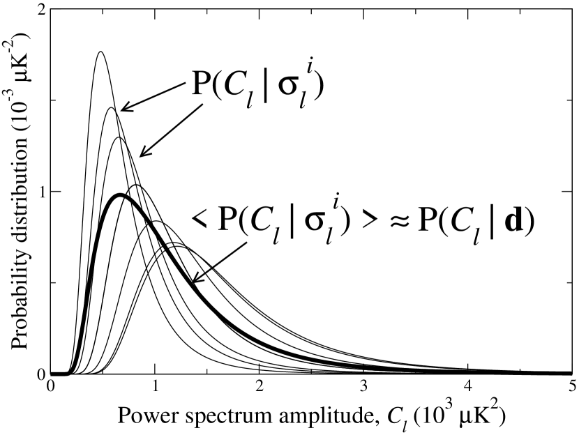
Figure 1: A one-dimensional illustration of the BR estimator. The thin lines indicate the $P(C_{\ell}|\sigma_{\ell}^{i})$ distributions, and the thick line shows their average. This average converges toward the true density $P(C_{\ell}|\mathbf{d})$ as the number of samples increases.

The expression in Eq. 11 is very useful because, for a Gaussian field,

$$P(C_{\ell}|\sigma_{\ell})\propto\prod_{\ell=0}^{\infty}\frac{1}{\sigma_{\ell}}\left(\frac{\sigma_{\ell}}{C_{\ell}}\right)^{\frac{2\ell+1}{2}}\,e^{-\frac{2\ell+1}{2}\frac{\sigma_{\ell}}{C_{\ell}}},$$ (12)

or

$$\ln P(C_{\ell}|\sigma_{\ell})=\sum_{\ell=0}^{\infty}\left(\frac{2\ell+1}{2}\left[-\frac{\sigma_{\ell}}{C_{\ell}}+\ln\left(\frac{\sigma_{\ell}}{C_{\ell}}\right)\right]-\ln\sigma_{\ell}\right),$$ (13)

up to a normalization constant. Eq. 13 is straightforward to compute analytically, and an arbitrarily exact representation of the posterior (with increasing $N_{\textrm{G}}$) may therefore be established conveniently by means of Eqs. 11 and 13.

II.3 Comparison with Brute-Force Likelihood Evaluation

In order to verify that the method works as expected, we apply it to a simulated map, and compare the results to a brute-force evaluation of the likelihood. Since this likelihood computation requires inversion of the signal plus noise covariance matrix, we limit ourselves to a low-resolution case, with properties similar to those of the COBE-DMR data (Bennett et al., 1996), but with significantly lower noise. Specifically, we simulate a sky using the best-fit WMAP power law spectrum, including multipoles between $\ell=2$ and 30. We then convolve this sky with the DMR beam, add 0.5% of the 53 GHz DMR noise (in order to regularize the covariance matrix as the beam drops off), and finally we apply the extended DMR sky cut.

Figure 2: Contours in $(q,n)$ space of constant probability given the simulated data described in text, for both the BR estimator (solid) and brute-force evaluation of the likelihood (dashed). Contours are where $-2\ln P(C_{\ell}|\textbf{d})$ rises by 0.1, 2.3, 6.17, and 11.8 from its minimum value, corresponding (for Gaussian distributions) to the peak, and the 1, 2 and 3$\sigma$ confidence regions.

 

(a) Convergence ratio $f=0.06$

(b) Convergence ratio $f=0.47$

Figure 3: Illustration of the convergence criterion defined by Eq. 15. If $f\equiv 0$, the two distributions overlap perfectly, while if $f\equiv 2$, then they are completely separated. The two distribution pairs shown here have $f=0.06$ and $f=0.47$, respectively.

This simulation is then analyzed both using the Gibbs sampling and BR machinery as described above, and by computing the full likelihood over a parameter grid using the Cholesky decomposition method of Górski (1994). The model power spectrum chosen for this exercise is of the form

$$C_{\ell}(q,n)=q\left(\frac{\ell}{\ell_{\textrm{0}}}\right)^{n}C_{\ell}^{\textrm{fid}},$$ (14)

where $q$ is an amplitude parameter, $n$ is a spectral index, $\ell_{\textrm{0}}$ is a reference multipole, and $C_{\ell}^{\textrm{fid}}$ is a fiducial power spectrum, which we take to be that of a flat $\Lambda$CDM model that fits the data well. The fiducial spectrum is chosen to be the input spectrum, and consequently, we should expect the likelihood of the parameters to peak near $(q,n)=(1,0)$.

The comparison between the brute-force evaluation and the BR approximation is not quite as straightforward as one would like. The problem lies in how to truncate the spherical harmonics expansion at high $\ell$’s. The brute-force likelihood computation requires that the full signal component is contained in the included harmonic expansion, which means that the noise power has to be larger than the convolved signal power before truncation. On the other hand, the Gibbs sampling approach requires a large number of samples to converge in this low signal to noise regime. The simulation was therefore constructed as a compromise: a very small amount of noise was added to make the covariance matrix well-behaved at the very highest $\ell$’s included, but not more than necessary. Still, small differences between the two approaches must be expected.

The results from this exercise are shown in Fig. 2. The contours show the lines of constant likelihood where $-2\ln P(C_{\ell}|\textbf{d})$ rises by 0.1, 2.3, 6.17 and 11.8 from the minimum, corresponding to the peak and the 1, 2, and $3\sigma$ regions for a Gaussian distribution. The solid lines show the results from the BR computation, and the dashed lines show the results from the exact likelihood computation. Obviously, the agreement between the two distributions is excellent, considering the very different approaches taken, and the above-mentioned high-$\ell$ truncation problem.

III Convergence of the BR estimator applied to WMAP data

The ultimate goal of this paper is to apply the methods described above to the first-year WMAP data. In order to do so, we first need to determine the accuracy of the BR estimator given our finite number of samples. In this section we do so by examining how the BR estimator fluctuates as different subsets of the Gibbs chains are used.

The Gibbs machinery was applied to the first-year WMAP data by O’Dwyer et al. (2004), and the primary results from that analysis were a number of $C_{\ell}$ and $\sigma_{\ell}$ sample chains. These chains are available to us, and form the basis of the following analysis. The data we use here are those computed from the eight cosmologically interesting WMAP Q-, V- and W-bands, comprising 12 independent chains of about 80 samples each for a total of 955 samples. For more details on how these samples were generated, we refer the reader to O’Dwyer et al. (2004) and Eriksen et al. (2004).

The main question we need to answer before proceeding with the actual analysis is, how well does this finite number of samples describe the full likelihood for a given range of multipoles? To answer this question, we define a simple test based on the $(q,n)$ model of Eq. 14 as follows: We construct two subsets from the 955 available samples, each containing $N_{\textrm{s}}<955/2$ samples, and map out the probability distribution for each subset, including only multipoles in the range $2\leq\ell\leq\ell_{\textrm{max}}$. From the two resulting probability distributions, $P_{1}(q,n)$ and $P_{2}(q,n)$, we compute the quantity

$$f=\frac{\int|P_{1}(q,n)-P_{2}(q,n)|\,\textrm{d}q\textrm{d}n}{\int P_{1}(q,n)\,\textrm{d}q\textrm{d}n},$$ (15)

which measures the relative normalized difference between the two distributions; if $f\equiv 0$ then the two distributions overlap perfectly, and if $f\equiv 2$, they are completely separated. We then increase $N_{\textrm{s}}$ until $f<0.05$ for the first time. Two sets of such distributions are shown in Fig. 3, having $f=0.06$ and $f=0.47$ respectively.

Of course, the chain is likely to go in and out of convergence as $N_{\textrm{s}}$ is increased further for quite some time, and therefore there will be a large random contribution to this particular statistic. For that reason we repeat the experiment eleven times, each time scrambling the full 955 sample chain, and define the median of the resulting $N_{\textrm{s}}^{i}$’s as the number of samples required for convergence. The process is then repeated for various values of $\ell_{\textrm{max}}$.

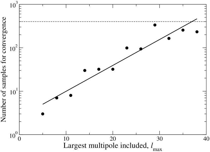
Figure 4: The number of samples required for convergence in the BR estimator of the first-year WMAP data, as defined in Section III. The dots indicate the results computed from the data as described in the text, while the solid line indicates a exponential best-fit. The dashed lines indicate the limit above which we cannot probe because of the limited number of available samples. For this calculation we chose $f=0.05$.

The results from this exercise are summarized in Fig. 4. Two important conclusions may be drawn from the information shown in this plot. First, the number of samples required for convergence increases very rapidly with $\ell_{\textrm{max}}$, possibly following an exponential. However, the fit is less than perfect, and the true function may possibly be steeper at the very smallest multipoles than the larger ones, which would be helpful when probing the higher $\ell$-range. Unfortunately, the limited number of available samples prohibits us from determining this function further.

Second, while it is strikingly clear from Fig. 4 that the existing number of samples is inadequate for probing the full multipole range properly, we may still conclude that the multipole range $2\leq\ell\leq 30$ is quite stable given that we have 955 samples. In the analysis described in the next section, we therefore construct a hybrid likelihood consisting of the BR likelihood for $\ell\leq 30$ and the analytic WMAP approximation at higher $\ell$’s.

A second demonstration of the same result is shown in Fig. 5, where we have computed the two-parameter likelihood using the BR estimator, splitting the sample chain into two parts, for three disjoint $\ell$-ranges ($\ell\in[2,12],[13,20]$ and $[21,30]$). Here we see that the estimator is very stable over each of the three $\ell$ ranges.

Figure 5: Constraints on $q$ and $n$ where $C_{\ell}(q,n)=q\,(\ell/\ell_{0})^{n}\,C_{\ell}^{\textrm{fid}}$ and $C_{\ell}^{\textrm{fid}}$ is a fiducial $\Lambda$CDM power spectrum for $\ell_{0}=8$, 17, and 25 from left to right. Solid lines are for one half of the BR samples and dashed lines are for another half. Contour levels are as in Fig. 2.

We have also considered the question of burn-in of the 12 independent sample chains, by repeating the analyses described above with reduced chains. Specifically, we removed the five or ten first samples from each chain, and repeated the analyses. Neither result changed as an effect of this trimming, implying that burn-in is not a problem for the Gibbs sampling approach at low $\ell$’s when the estimated WMAP spectrum is used to initialize the Gibbs chains. This result is in good agreement with the results presented by Eriksen et al. (2004), who showed that the correlation length of the Gibbs chain is virtually zero when the signal-to-noise is much larger than one.

IV Blackwell-Rao vs. WMAP $P(C_{\ell}|\mathbf{d})$

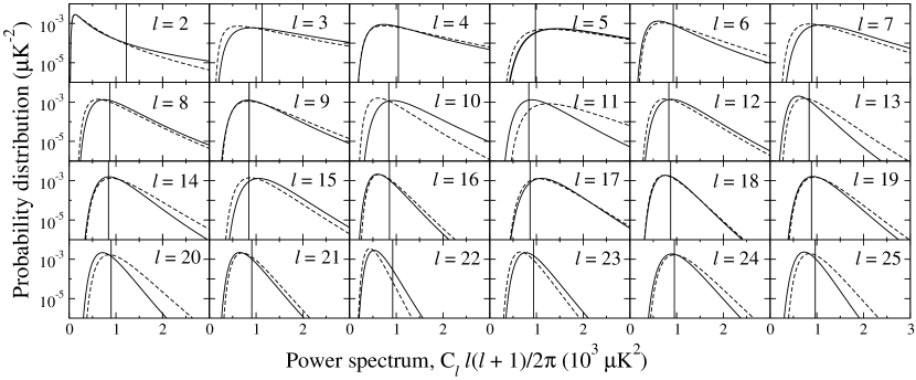
Figure 6: Comparison of the BR (solid curve) and the analytic WMAP (dashed curve) univariate likelihood functions for each multipole up to $\ell=25$. The vertical lines indicates the value of the best-fit WMAP power-law model (not including a running spectral index). The univariate likelihood functions are computed by slicing through the multivariate likelihood, fixing all other multipoles at the corresponding best-fit value. Notice that all distributions shown here are strongly non-Gaussian.

There are a number of differences between our analysis and the WMAP team’s analysis. Here we examine the resulting differences in $P(C_{\ell}|\mathbf{d})$ and in the next section on estimates of cosmological parameters. Our goal is to understand the significance of these low $\ell$ differences. We do not attempt to completely disentangle which $P(C_{\ell}|\mathbf{d})$ differences are due to which analysis differences.

There are at least four areas where the WMAP team’s analysis differs from ours:

1. They use a pseudo-$C_{\ell}$ technique to estimate the most likely $C_{\ell}$;

2. At $\ell<100$, in order to reduce residual foreground contamination they do not include Q-band data;

3. Their pseudo-$C_{\ell}$ estimate places zero weight on the auto-correlation of maps from the individual differencing assemblies; and,

4. They use a variant of the analytic approximation of Bond et al. (2000) to the shapes of the likelihoods.

A number of these differences in analysis procedures were discussed by H03 and Verde et al. (2003). Regarding item 1, one can see in H03 Fig. 12 differences at low $\ell$ between a maximum-likelihood analysis and pseudo-$C_{\ell}$ analysis as applied to V-band data. Regarding item 2, in Fig. 3 of H03 one can see differences at low $\ell$ between inclusion and exclusion of the Q-band data. Regarding item 3, one can see differences at low $\ell$ in Fig. 6 of H03 depending on whether the auto-correlations are included.

The net result of all these effects is shown in Fig. 6 and 7. In Fig. 6, we compare the univariate likelihood functions for all multipoles up to $\ell=25$, as computed using both the WMAP analytic approximation (dashed smooth line) and the BR approximation (solid smooth line). The BR likelihoods are computed by varying one single multipole at a time, keeping the other multipoles fixed at the best-fit power-law model value.

There are a few clear differences between the two sets of distributions shown in Fig. 6, the most prominent being a small horizontal shift in most cases, or in other words, different power spectrum estimates. This was anticipated, given the differences discussed above.

More important than these shifts are the relative shapes of the two distributions. Such features are most easily compared when the two distributions have identical modes, which is the case for $\ell=2,4,9$ and 14. In the quadrupole case we see that the BR distribution has a heavier tail than the WMAP distribution, while the opposite is true for the other three cases. On the other hand, we find spectacular agreement for the $\ell=17$ and 18 cases. All in all, the results shown in this figure are consistent with the idea that the Gibbs sampling approach is an optimal method, while the WMAP approach is based on a pseudo-$C_{\ell}$ method, and the latter is therefore expected to have slightly larger error bars. The only case for which this rule is obviously broken is the quadrupole, and thus we have reason to question the accuracy of this particular multipole.

We also note that a similar analysis was carried out by Slosar et al. (2004). One of their major results was a significantly broader likelihood than the WMAP likelihood (as well as a strong shift toward larger amplitudes) for $\ell\leq 10$. The main difference between that analysis and the present is that they marginalized over three foreground templates, and, given the results shown in this section, this additional degree of freedom is most likely the cause of the broadened likelihood, rather than inherently under-estimated errors in the WMAP likelihood code. Slosar et al. (2004) also found a coherent shift toward larger amplitudes. We see this ourselves to a lesser degree in Fig. 6. Seven out of the eleven $C_{\ell}$ in the $\ell=2$ to 12 range show some amount of shift to higher $\ell$.

To further study the differences in $P(C_{\ell}|\mathbf{d})$ between the BR approximation and the analytical approximation used by the WMAP team, we once again adopt the two-parameter non-physical model defined in Equation 14, $C_{\ell}(q,n)=q\left(\ell/\ell_{0}\right)^{n}C_{\ell}^{\textrm{fid}}$, and map out in Fig. 7 the two likelihoods in $q$ and $n$ using the two approximations. We display these likelihoods over the same $\ell$ ranges as in Fig. 5. We can see in the left panel (the $\ell=2$ to 12 range) clear evidence for a shift to higher power hinted at by the individual multipole distributions in Fig. 6. The peak shifts by $\sim 3/4\sigma$ and the BR contours are slightly tighter than the WMAP ones. Discrepancies are smaller in the $\ell=13$ to 20 range and smaller still in the 21 to 30 range, especially near $n=0$. Note that the likelihood at $|n|\mathrel{\mathchoice{\lower 3.6pt\vbox{\halign{$\mathsurround=0pt\displaystyle\hfil#\hfil$\cr>\crcr\sim\crcr}}}{\lower 3.6pt\vbox{\halign{$\mathsurround=0pt\textstyle\hfil#\hfil$\cr>\crcr\sim\crcr}}}{\lower 3.6pt\vbox{\halign{$\mathsurround=0pt\scriptstyle\hfil#\hfil$\cr>\crcr\sim\crcr}}}{\lower 3.6pt\vbox{\halign{$\mathsurround=0pt\scriptscriptstyle\hfil#\hfil$\cr>\crcr\sim\crcr}}}}1$ is irrelevant for physical models since their spectral shapes do not deviate that strongly from that of the fiducial.

Figure 7: Constraints on $q$ and $n$ where $C_{\ell}(q,n)=q\,(\ell/\ell_{0})^{n}\,C_{\ell}^{\textrm{fid}}$ and $C_{\ell}^{\textrm{fid}}$ is a fiducial $\Lambda$CDM power spectrum for $\ell=2$ to $\ell=12$ with $\ell_{0}=8$ (left panel), $\ell=13$ to $\ell=20$ and $\ell_{0}=17$ (center panel) and $\ell=21$ to $\ell=30$ with $\ell_{0}=25$ (right panel). Solid lines are for BR and dashed lines are for the WMAP likelihood code. Contour levels are as in Figure 2.

To summarize this section, we have seen that the BR estimate and that of WMAP for $P(C_{\ell}|\mathbf{d})$ do differ slightly at low $\ell$’s. This should result in differences in parameter estimates, to which we now turn.

V Effect on cosmological parameters

We now explore how significant these low $\ell$ differences are for estimates of cosmological parameters. We consider two different cosmological model parameter spaces. The first is a flat $\Lambda$CDM cosmology with a power-law primordial power spectrum. The second parameter space allows for a logarithmic scale-dependence to the power-law spectral index so that $n_{\textrm{s}}(k)=n_{\textrm{s}}(k_{0})+\textrm{d}n_{\textrm{s}}/\textrm{d}\ln k\ln(k/k_{0})$. The $\textrm{d}n_{\textrm{s}}/\textrm{d}\ln k$ parameter is commonly referred to as the ‘running of the spectral index’, a reference to the analogous dependence of gauge coupling strength with energy scale in quantum field theories.

We explore the parameter spaces via the MCMC mechanism as described by, e.g., Christensen et al. (2001). For the 6-parameter cosmological models we use $\omega_{\textrm{b}}$, $\omega_{\textrm{d}}$, $\Omega_{\Lambda}$, $z_{\textrm{rei}}$, $A$, $n_{\textrm{s}}$ (baryon density, cold dark matter density, dark energy density, redshift of reionization, amplitude of the primordial power spectrum at $k=0.05\,{\rm Mpc}^{-1}$ and the scalar index; the total matter density is $\omega_{\textrm{m}}=\omega_{\textrm{b}}+\omega_{\textrm{d}}$) and a calibration parameter for each of CBI (Pearson et al., 2003) and ACBAR (Dickinson et al., 2004; Rebolo et al., 2004). For the 7-parameter cosmological model we use the the same six parameters plus $\textrm{d}n_{\textrm{s}}/\textrm{d}\ln k$. We evaluate the likelihood given the WMAP data with the subroutine available at the LAMBDA data archive. For CBI and ACBAR we use the offset log-normal approximation of the likelihood (Bond et al., 2000). The likelihood given all these data together (referred to as the WMAPext dataset by Spergel et al. (2003)) is given by the product of the individual likelihoods. For the the hybrid schemes, we replace the the WMAP likelihood calculation for the temperature power spectrum in the range $2\leq\ell\leq 30$ with the BR estimator. In all cases, we employ a prior that is zero except for models with $0.40<h<0.95$, $\tau<0.30$, and $6.0<z_{\textrm{rei}}$ (Fan et al., 2002) in which case the prior is unity. All chains have 100,000 samples.

	$\textrm{d}n_{\textrm{s}}/\textrm{d}\ln k$ fixed to zero			$\textrm{d}n_{\textrm{s}}/\textrm{d}\ln k$ free to vary
Parameter	WMAP $P(C_{\ell}|\mathbf{d})$	hybrid	difference/$\sigma$	WMAP $P(C_{\ell}|\mathbf{d})$	hybrid	difference/$\sigma$
$n_{\textrm{s}}$	$0.97\pm 0.03$	$0.97\pm 0.03$	0.0	$0.880\pm 0.048$	$0.903\pm 0.047$	0.4
$\tau$	$0.132^{+0.097}_{-0.048}$	$0.140^{+0.080}_{-0.053}$	0.1	$0.202\pm 0.065$	$0.208\pm 0.063$	0.1
$A$	$0.80\pm 0.10$	$0.79\pm 0.10$	0.1	$0.91\pm 0.11$	$0.90\pm 0.11$	0.1
$\omega_{\textrm{b}}$	$0.023\pm 0.001$	$0.023\pm 0.001$	0.0	$0.0215\pm 0.0013$	$0.0219\pm 0.0012$	0.3
$\omega_{\textrm{m}}$	$0.136\pm 0.014$	$0.132\pm 0.013$	0.3	$0.140\pm.015$	$0.134\pm 0.014$	0.4
$h$	$0.72\pm 0.05$	$0.73\pm 0.05$	0.2	$0.682\pm 0.054$	$0.708\pm 0.054$	0.5
$\textrm{d}n_{\textrm{s}}/\textrm{d}\ln k$	—	—	—	$-0.079\pm 0.031$	$-0.063\pm 0.031$	0.5

Table 1: Cosmological parameter means and standard deviations derived from the WMAPext dataset using the WMAP likelihood code (columns 2 and 5) and using our hybrid approach where the WMAP likelihood code for the tempearture angular power spectrum is replaced at $\ell\leq 30$ with our BR estimate of $P(C_{\ell}|\mathbf{d})$. The columns labeled ‘difference/$\sigma$’ give the difference in the parameter means divided by the standard deviation of the hybrid method. Note that the finite number of chain samples gives rise to an uncertainty in each mean of $\sim 0.1\sigma$.

The results for the 6-parameter case using the WMAP likelihood code (column 2 of the table) reproduce those reported by Spergel et al. (2003). We see that the hybrid scheme leads to almost no differences, with any shifts in most likely values smaller than $1/3\sigma$. Thus there is only a very weak dependence on the differences in $P(C_{\ell}|\mathbf{d})$ at low $\ell$. The reason for this is that with the 6-parameter model the data at high $\ell$ tightly constrain the range of $C_{\ell}$ values at low $\ell$.

Now we turn to the difference between columns 4 and 5, where the only difference in their derivation is the treatment of the temperature power spectrum at $\ell\leq 30$. With the extra freedom in the 7-parameter model, the high $\ell$ data can no longer be extrapolated to low $\ell$ with as much confidence. The data at low $\ell$ are thus more informative than in the six-parameter case and the differences at low $\ell$ become more important. Four parameters show shifts greater than $1/3\sigma$: $n_{\textrm{s}}$, $\omega_{\textrm{b}}$, $\omega_{\textrm{m}}$ and $\textrm{d}n_{\textrm{s}}/\textrm{d}\ln k$. The biggest shift is in $\textrm{d}n_{\textrm{s}}/\textrm{d}\ln k$. It reduces a $2.5\sigma$ detection to a 2$\sigma$ detection.

We checked to make sure these shifts are significant, given our limited number of chain elements. To do so, we looked at 4 subsamples of the 7-parameter case chains, each with 25,000 samples, to examine fluctuations in the subsample mean values of each parameter. We found these subsample means to deviate from the total sample means with an rms of $\sim 0.2\sigma$. We thus estimate the sample variance error in our sample means to be $\sim 0.1\sigma$. We also ran a chain with 100,000 samples with the switch at $\ell=20$, and found it to be consistent with the hybrid chain with the switch at $\ell=30$.

The direction of the changes is consistent with Fig. 7. We see our own analysis has a higher level of power and lower level of tilt in the $\ell=2-12$ range and is more restrictive of upward power fluctuations in the $\ell=13-20$ range compared to the WMAP team’s analysis. Thus we want the model power spectra to be more negatively sloped at low $\ell$. This is accomplished by the 0.026 increase in the running which reduces $n_{\textrm{s}}(k)$ at $k=0.009\,Mpc^{-1}$ (which projects to $\ell=12$) by 0.11 from its value at $k_{0}=0.05\,\textrm{Mpc}^{-1}$.

It should be noted that the parameter values are strongly dependent on the high $\tau$ cut. In fact we have found that most of the probability is at $\tau>0.3$, as has been noticed for WMAP + VSA (Rebolo et al., 2004; Slosar et al., 2004) and for WMAP+CBI (Readhead et al., 2004). At these high $\tau$ values, the running tends to be negative also. Having high $\tau$ and a negative running though is a priori unlikely in hierarchical models of structure formation, and is also disfavored when large-scale structure data is included (Slosar et al., 2004).

VI Extending BR to higher $\ell$’s

We face two challenges to extending the BR estimator to higher $\ell$ values. The first is that the greater the range of $\ell$ values, the greater the volume of parameter space to be explored (in units of the width of the posterior in each direction) and therefore the larger the number of samples required. The second is that as the signal-to-noise ratio drops below unity, the correlation length of the Gibbs samples, produced by the algorithms of Wandelt et al. (2004) and Jewell et al. (2004), starts to get very long thereby reducing the effective number of independent samples. We do not address this second problem here, which becomes important around $\ell\sim 350$, except to say that we are currently implementing potential solutions.

We see evidence of the first problem in Fig. 4. Here we discuss two solutions, both of which rely on the low level of dependencies between the errors in $C_{\ell}$ at different $\ell$ values. For the first solution, we replace the BR estimate with a ‘band BR’ estimate where the averaging over samples is done in discrete bands of $\ell$ that are then multiplied together. Specifically,

$$P(\{C_{\ell}\}|\mathbf{d}) = \Pi_{B}\langle P\left(C_{l_{<}(B)},C_{l_{<}(B)+1}...,C_{l_{>}(B)}\right.$$ (16)

$$\left.|\sigma^{i}_{l_{<}(B)},\sigma^{i}_{l_{<}(B)+1}...,\sigma^{i}_{l_{>}(B)}\right)\rangle$$

where $\langle...\rangle$ indicates averaging over samples and the lower and upper $\ell$ values of each band $B$ are denoted by $\ell_{<}(B)$ and $\ell_{>}(B)$.

The advantage of the band BR estimator is that it reduces the volume of the space to be explored from one with $\ell_{\rm max}-\ell_{\rm min}+1$ dimensions to a product over spaces with number of dimensions equal to the width of the bands, greatly reducing the volume in units of the extent of the posterior. The approximation here ignores inter-band dependencies. Tests though have shown these to be negligibly small for bands of width 12.

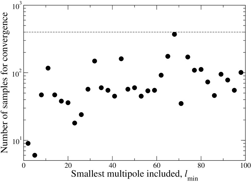
Figure 8: The number of samples required for convergence for the band BR estimator of the first-year WMAP data, as defined in Section III for bands extending from $\ell_{\rm min}$ to $\ell_{\rm min}+11$. The dots indicate the results computed from the data.

To demonstrate the reduction in the number of samples necessary for convergence, we re-do Fig. 4. In Fig. 4 $\ell_{\rm min}$ was fixed to 2 as $\ell_{\rm max}$ increased. Here as $\ell_{\rm max}$ increases so does $\ell_{\rm min}$ so that $\ell_{\rm max}-\ell_{\rm min}+1=12$. We see in Fig. 8 that switching to the band BR estimator flattens out the trend of necessary number of samples with $\ell_{\rm max}$.

It may be possible to exploit the near-independence of different $\ell$ values further. We can use BR (or even a fit to the histogram of $C_{\ell}$ values in the chain) to estimate univariate marginalized distributions, multiply these together as if they were independent, and then correct for the correlations with an analytic correction factor. Namely,

$$\ln P(\{C_{\ell}\}|\mathbf{d}) = \sum_{\ell}\ln\left(P(C_{\ell}|\mathbf{d})\ \right)$$ (17)

$$+ \sum_{\ell}\frac{\delta C_{\ell}^{2}}{2C_{\ell\ell}}-\sum_{\ell,\ell^{\prime}}\delta C_{\ell}F_{\ell\ell^{\prime}}\delta C_{\ell^{\prime}}/2$$

where $\delta C_{\ell}\equiv C_{\ell}-\langle C_{\ell}\rangle$, $F_{\ell\ell^{\prime}}$ is the $C_{\ell}$ Fisher matrix and $C_{\ell\ell^{\prime}}$ is its inverse. These matrices can be computed as in H03. Note that the above expression is exact for a Gaussian distribution, with the first term in the log of the correction factor simply canceling out the sum of the logs of the marginalized one-dimensional distributions. Such a procedure will only require a handful of independent samples. Further, one could combine our two solutions here by using band BR with an analytic correction for the neglected inter-band dependencies.

Certainly this use of analytics could be extended further to reduce the demand for number of independent samples. We expect that an adequate analytic form can be found for the posterior. One would then use the BR estimator, or the $C_{\ell}$ samples, to fit the parameters of this analytic form. Such an approach could greatly reduce the demand for the number of independent samples. Essentially, we would be exploiting the fact that $P(\{C_{\ell}\}|\mathbf{d})$ is a very smooth distribution with a lot of regularity, such as the structure of inter-$\ell$ correlations and shapes of univariate distributions. Such an approach will probably be necessary in the high $\ell$ regime where larger correlation lengths (at least for current sampling techniques) greatly reduce the number of independent samples.

In the low signal-to-noise regime the number of independent samples required, even to explore the posterior for a single $\ell$ value, increases because the width of the BR estimator from an individual sample is much smaller than the width of the posterior (since the former is for a noiseless sky). This problem can be mitigated by artificially broadening the BR kernel. Specifically, we would set

$$\ln\left(P\left(C_{\ell}|\sigma_{\ell}\right)\right) = \frac{n_{\ell}}{2}\left[-\frac{\sigma_{\ell}}{C_{\ell}}+\ln\left(\frac{\sigma_{\ell}}{C_{\ell}}\right)\right]-\ln(\sigma_{\ell})$$

$${\rm and\ \ }n_{\ell} \equiv (2\ell+1)\left(1+\alpha N_{\ell}/C_{\ell}\right)^{-2}$$ (18)

where $N_{\ell}$ is the noise contribution to the power spectrum of the map. Setting $\alpha>0$ broadens the kernel for each sample from $\propto C_{\ell}$ to $\propto(C_{\ell}+\alpha N_{\ell})$. Unfortunately it also broadens the posterior from $\propto(C_{\ell}+N_{\ell})$ to $\propto\left(C_{\ell}+(1+\alpha)N_{\ell}\right)$. Thus one must choose $\alpha$ small enough so the posterior is not overly broadened. At high $C_{\ell}/N_{\ell}$ this broadening makes no difference. At low $C_{\ell}/N_{\ell}$ the sample kernel is broadened by a large factor ($1+\alpha N_{\ell}/C_{\ell}$) while the posterior is broadened only by 1+$\alpha$. Thus one can broaden the sample kernel in the low signal-to-noise regime (exactly where we want to broaden it) by a very large amount, without significantly broadening the posterior. The number of independent samples required for convergence will drop by this same factor.

Finally, we mention one more way to reduce the dimensionality of the space to be explored, and thus the number of samples required. And that is to replace the $C_{\ell}$’s with band powers. In the low signal-to-noise regime such a replacement need not lead to significant loss of information, assuming models with smooth $C_{\ell}$’s.

VII Conclusions

We have found BR to be a useful step in the process of converting CMB anisotropy data, and a model of it, into estimates of $P(C_{\ell}|\mathbf{d})$. We have shown that precise characterization of this distribution at low $\ell$ is a key step in the estimation of cosmological parameters. The differences between $P(C_{\ell}|\mathbf{d})$ as computed by us with a hybrid approach that uses BR at $\ell\leq 30$ and as computed by the WMAP team can lead to important differences in estimates of cosmological parameters.

The BR estimator converges rapidly at low $\ell$, but requires many independent samples at high $\ell$. By exploiting the weak inter-$\ell$ dependence in $P(C_{\ell}|\mathbf{d})$ we were able to modify the BR estimator to greatly improve convergence without significantly sacrificing accuracy. Extensions that will allow its use with correlated data, such as temperature and polarization, or weak lensing shear from multiple redshift bins, and to higher $\ell$ are worth pursuing.