Initial results from SECIS observations of the 2001 eclipse

Abstract

SECIS observations of the June 2001 total solar eclipse were taken using an Fe xiv 5303 Å filter. Automated tools based on wavelet analysis was used to detect intensity oscillations on various areas of the images. Statistical analysis of the detections found in the areas covered by the moon and the upper corona allowed us to estimate the atmospheric and instrumental effects on the detection of intensity oscillations. An area of the lower corona, close to Active Region 9513, was found with a statistically significant amount of intensity oscillations with periodicity of $\sim$7.5$s$. The shape of the wavelet transformation of those detections matches theoretical predictions of sausage-mode perturbations and for the first time in the SECIS project, second order oscillations were also detected.

1 Introduction

The magnetohydrodynamic (MHD) waves in corona loops have been investigated as a possible cause of coronal heating by numerous authors. Hollweg [1] first proposed a mechanism that involved MHD waves dumping their energy into the solar corona through ion viscosity and electrical resistivity, while other authors favoured magnetic reconnection followed by current dissipation (for example Parker [2]). Priest & Schrijver [3] have recently published a review article that contains all the theoretical attempts and their limitations.

MHD oscillations are usually divided in two main categories depending on the presence or not of density perturbations. Magnetoacoustic MHD waves are defined as the density, pressure and temperature perturbations (which are in turn divided into slow and fast modes), while the incompressible waves are called Alfvén and are also divided into those with movements perpendicular to the magnetic field and torsional. Roberts et al. [4] study a low-$\beta$ plasma, using reasonable values for the solar corona approximations and predicted that fast magnetoacoustic (sausage-mode) oscillations with frequencies around 1 Hz can be excited in coronal loops. They also study the signature of a wave train, created by a pulsation at $x=0$ observed at a point $x=x^{\prime}$. Much later, Nakariakov et al. [5] used numerical analysis to confirm the initial study and provide a more accurate simulation.

The Solar Eclipse Coronal Imaging System (SECIS) is an eclipse imager that was developed specifically to detect corona oscillations, following a long history of similar attempts (Koutchmy et al. [6], Pasachoff & Landman [7], Singh et al. [8], Cowsik et al. [9], Pasachoff et al. [10]). An Fe xiv 5303 Å filter was used by the SECIS project to observe the August 1999 and June 2001 total solar eclipses and the results of the 1999 observations were reported in a sequence of papers (Williams et al. [11], Williams et al. [12], Katsiyannis et al. [13]), while a detailed description of the instrument is provided by Phillips et al. [14]. [11], [12] and [13] consistently detected several periodicities in the range of 4-7 s, while [12] reported a propagating wave train travelling through the corona loop with a phase-speed of $\sim$2100 km s^-1, making a fast-mode MHD wave as the most likely explanation of the observed intensity perturbation. By working on a different loop of the same active region [13] found intensity oscillations just outside but fully aligned with visual corona loops. Their detections were in the same frequency range and have similar amplitudes as with [11] and [12]. After calculating the physical characteristics of the loop (physical dimensions, density, etc) and with reasonable assumptions regarding the strength of the magnetic field, Roberts (private communication) confirmed that the frequencies reported by the above authors ([11], [12] and [13]) are well within the range predicted by [4].

Following the observations, reduction and data analysis of the 2001 eclipse were reported by Katsiyannis et al. [15]. In this paper we will present further progress in the analysis of the data, a detailed statistical analysis of the effects of the earth’s atmosphere and some preliminary detections of oscillations in the lower solar corona.

2 Observations

An analytical description of the observations taken by SECIS during the August 1999 total solar eclipse is presented by [14]. Although the SECIS total solar eclipse observations of 2001 are described in detail by [15], a briefer description of these observations is presented in this section for clarity. In particular, the alterations made to the instrument and some of the characteristics and specifications will be presented below.

• The green Fe xiv 5303 Å filter used in the previous eclipse was replaced with a broader, also Fe xiv 5303 Å filter, centred at practically the same line. The new filter has a full-width-half-maximum (FWHM) of 5 Å while the old filter was just 2 Å.

• A metallic encloser was used to cover the optical elements of SECIS and reduce the amount of scattered light. The whole optical path from the back of the Schmidt telescope to the charge-coupled device (CCD) cameras was covered by this cover. A detailed diagram of the instrument and the optical path covered can be found in [14].

• Instabilities of the rotation axis speed of the heliostat have been observed by [14]. As a possible cause of those instabilities is contamination of the driving mechanism of the heliostat, a cover was produced that protected the area from dust. The analysis of the data that followed showed no repeat of the 1999 instabilities on the 2001 observations.

• The CCD cameras were cooled by newly installed fans, reducing the thermal effects.

The 21^st of June 2001 total solar eclipse was observed following similar procedure to the August 1999 experiment. The instrument was transfered in parts and was assembled on the the roof of the Physics department of the University of Zambia, in Lusaka, Zambia (Latitude: 15^∘ 20^′ South; Longitude:28^∘ 14^′ East). The optical components of the instrument were aligned using a pocket laser while the heliostat and the optical axis of the instrument were aligned with the solar path using the standard gnome technique. Distant objects were used for the focusing of the various optic components.

During the eclipse weather conditions were good with practically no wind or clouds. The cooling fans of the CCD cameras were switched on early on the day of the eclipse but were switched off a few minutes before totality to avoid vibrations to the instrument. The two identical CCD detectors have 512 $\times$ 512 pixels, which combined with the optics of the instrument provide us with an observable area of $\sim$ 34$\times$34 arcmin² and a resolution of 4 arcsec pixel^-1 (see [11] and references therein). Due to edge effects and localised thermal effects on the CCD, an area of $\sim$ 400 $\times$ 300 pixels was used for the data analysis. Also the first 1000 frames of the data set were not used in any part of the analysis described below as they were effected by light from the photosphere during the start of the eclipse (an effect also known as “diamond rings effect”). Having a previous knowledge of the limitations of the CCD on the observable area and in line with practice followed during the 1999 eclipse, the observations were not centred at the centre of the disk but close to the North-East limb. This location was chosen because of the appearance of NOAA Active Region 9513 off the limb of the disk on the previous day. 8000 images were obtained during totality by the SECIS instrument with a cadence of 39 frames per second, so the whole duration of the totality was covered. The same area of the Sun was observed also by the Solar and Heliospheric Observatory (SoHO) during totality so the physical characteristics of AR 9513 can be determined.

Sky flat fields and dark frames (flats and darks for short) were obtained the next morning. The same exposure time with the eclipse observations was used for both the flats and the darks. For the flat fields the heliostat was turned towards a featureless part of the sky, while for the dark frames the apertures of the two lenses were closed to f/22 and the cameras were covered completely with a black cloth.

3 Data Reduction and Analysis

The data reduction software developed for the analysis of the 2001 eclipse data is described in detail by [15]. Since then various improvements were made mostly to the way the images were aligned. A brief description of the whole reduction and analysis is below and the differences with [15] will be explicitly mentioned.

3.1 Image Alignment

In a first stage dark current and sky flat subtraction was performed in the standard way for astronomical images.

The second phase involved alignment of the 8000 images to an accuracy of one pixel.

The third step was the 8000 images to be aligned with an accuracy of 1 pixel. This was a different goal to what [15] tried to achieve as later test revealed that the sub-pixel accuracy may introduce artificial oscillations. The first step of the alignment procedure was to use the Sobel filter to calculate the edge of the moon disk and then, assuming a constant lunar radius, a fit of the disk was produced and compared with the edge fitted by the Sobel function. Those points that were lying outside the fit by more than 3$\sigma$ were rejected. In the next step we assumed that the centre of the moon was moving in respect to the Sun with a constant velocity and the images were corrected for this effect. In the final stage further accuracy was achieved by using an area of the 1000^th image containing featureless parts of corona as well as a sharp transition from the moon disk as a reference. This area was correlated with the equivalent areas of the rest of the 8000 images and the pixel shifts for which this correlation was maximum were considered the final shifts for the alignment of the images. Unlike the procedure followed by [15], there was no expansion of the correlation area.

3.2 Wavelet analysis

In line with previous work on SECIS ([11]-[13] and [15]) continuous wavelet analysis was used to detect intensity oscillations. This choice was made mainly because coronal loop oscillations are not expected to necessarily last more than a few periods which meant that a technique that produces the power of an oscillation over the whole length of the experiment (like Fourier analysis) would be unsuitable. As practically all the detections of intensity oscillations done by SECIS have periods on the region of $\sim$5 to 8$s$, while the time series are either 40$s$ (1999 data set) or 205$s$, none of the detections reported by [11], [12] and [13] would had been possible if Fourier analysis was used.

Torrence & Compo [16] describe in detail the algorithm used and provide a discussion of its benefits and application on various scientific problems. A very brief description of the transformation follows below for completeness.

$$\psi(\eta)=\pi^{-1/4}\exp(i\omega_{0}\eta)\exp(\frac{-\eta^{2}}{2}),$$

where $\eta=t/s$ is the dimensionless time parameter, t is the time, s the scale of the wavelet (i.e. its duration), $\omega_{0}=s\omega$ is the dimensionless frequency parameter, and $\pi^{-1/4}$ is a normalisation term (see [16]).

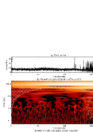
Figure 1: Wavelet transform analysis of point x=374, y=211 of the aligned data set. Panel (a) contains the time series while (b) is the wavelet transform. The contours in panel (b) highlight the areas where the detected power is at the 99% confidence level and the hatched area is the cone-of-influence (COI).

The results of the wavelet analysis described above applied to pixel x=374, y=211 of the aligned 2001 data set are shown on Figure 1. Panel (a) is a plot of the time series of pixel x=374, y=211 of the aligned data. Panel (b) displays the power density wavelet transform of the above time series with the lighter areas representing the higher values. The hatched region marks the cone-of-influence (COI) and represents the areas that suffer from edge effects. Everything inside the COI should be discarded. More details on the edge effects introduced by a finite time-series and how the hatched area is affected by this can be found in [16] and the references their in. The contours of panel (a) surround the area where the detected power exceeds the 99% confidence level.

4 Automated Detection of Oscillations

Software for the automated detection of intensity oscillations on the SECIS data set was developed by [15] and was extensively used for this study also. As with [15] this was done due to the large number of pixels included in the data set. In total 5400 pixels were passed through the scanning program for the determination of atmospheric and instrumental effect and the detection of lower corona loop oscillation (for more details see sections 5 and 6).

The following criteria were applied for the detections to be considered valid. Both the choice of the mother wavelet and the selection criteria were chosen for consistency with previous work by [12], [13] and [15]. See [13] for a detailed discussion on the establishment of these criteria.

• All values of coefficients falling within the COI are discarded.

• Only areas with 99% confidence level or higher are taken into account.

• All oscillations lasting less than the time length of three periods were discarded.

A brief description of the software, written in IDL, follows:

1. For a given pixel of the data set the continuous wavelet coefficients of the time series was produced.

2. For the lowest periodicity the number of the first sample in time that is unaffected by the COI is determined. This sample is called ${\rm t}$.

3. For the same periodicity the last sample that is unaffected by the COI, ${\rm t^{\prime}}$, was calculated.

4. The number of the sample that predates ${\rm t^{\prime}}$ by three periodicities is determined. This sample is called ${\rm t}_{\mathrm{m}ax}$

5. The confidence level of the sample ${\rm t}$ is calculated

6. If the confidence level of sample ${\rm t}$ is 99% or higher, then the confidence level of the sample that is three periods later, say ${\rm t_{+3}}$, is also extracted. Otherwise we go to step 8.

7. If the confidence level of ${\rm t_{+3}}$ is also 99% or higher the co-ordinates of the pixel, the current periodicity and ${\rm t}$ are recorded. In this case the algorithm goes to step 9. In this point, it is assumed that if ${\rm t}$ and ${\rm t_{+3}}$ have both confidence level of 99% or higher, all samples between them will have confidence level of 99% or higher in the same periodicity. This assumption is rarely wrong. All automated detections we have ever inspected manually fulfil this hypothesis.

8. Go to the next ${\rm t}$ and repeat steps 5-7 until ${\rm t}$ becomes ${\rm t_{max}}$.

9. Go to next periodicity and repeat steps 2-8 until the periodicity reaches the limit of 70.9 $s$.

10. Move to the next pixel of the array and start again the entire procedure.

70.9 $s$ is the upper limit of periodicities that can be detected in the SECIS 2001 data set. This is because any oscillations with longer periods do not have a long enough part of the time series outside the COI to satisfy the criteria mentioned above.

5 Atmospheric and Instrumental effects

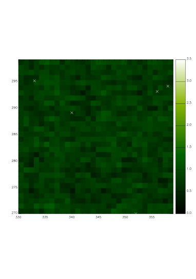
Figure 2: A 30$\times$30 pixels area covered by the Moon. Out of the 900 pixels, 5 were found to oscillate with a periodicity of 7-8 $s$. The pixels where those oscillations were found, are marked with ‘x’. On average, the chance of a pixel of this area to be found to oscillate is 0.56%.

Each frame of the SECIS eclipse observations can be divided into three parts. The first is the area covered by the moon disk and contains only signal from scattered line from the Earth’s atmosphere. The second part has signal mainly from the solar corona and the third part is dominated by light coming from the outer corona.

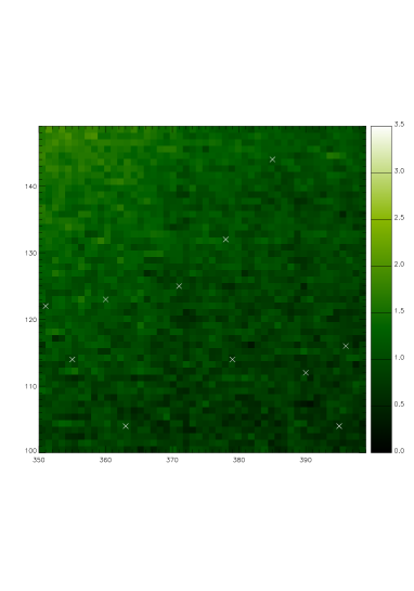
Figure 3: A 50$\times$50 pixels area of the upper corona. Out of the 2500 pixels, 11 were found to oscillate with a periodicity of 7-8 $s$. On average, the chance of a pixel of this area to be found to oscillate is 0.44%.

The different properties of these three areas are used in order to estimate the atmosphere and instrumental effects to the detection of intensity oscillations. The automated method and the criteria for detecting oscillations, as defined in the previous sections, were applied to a sample area of the moon and the outer corona. Figures 2 and 3 contain the averaged, over the whole time sequence, images of an area of the moon and outer corona respectively. The two axes of both images are the pixel coordinates of the aligned data set and the green scale are the average pixel values. Both areas were chosen to be close to AR 9513 but significantly distant to the edge of the moon (for the disk sample) and the edges of the useful area (for the outer corona sample).

When applied to the sample moon area, for the detection of oscillations with 7-8$s$ periodicity, the automated software produced 5 detections of oscillations out of 900 pixels. Since no signal from the lower corona is detected in this area directly, all counts generated will be either CCD read-out noise, or scattered atmospheric light. When different ranges of periodicity are scanned by the same software in the same area different pixels in random locations are found to oscillate. This led us to believe that the moon detections behave randomly and normal statistical procedures can be used to determine the atmospheric and instrumental effects. Further verification of this assumption is provided by the 50$\times$50 area of the outer corona displayed in Figure 3. Using the same software, 11 oscillations were found in the same periodicity range, making the average possibility of a pixel of this coronal area to found with intensity oscillations 0.44%. This is very close to 0.56% for the moon area reported above and confirms our assumption that the intensity oscillation in the outer corona are too weak for SECIS to detect them. Therefore any oscillations found in the upper are mostly due to atmospheric and instrumental effects. To provide further confirmation to this assumption more sample areas will be used from both the lunar disk and outer corona areas and the possibility of a pixel to oscillate will be calculated for each sample area separately. The standard deviation of this measurements will provide us with an estimation of how consistent the atmospheric and instrumental effects are throughout the data set.

6 Detections of Oscillations around AR 9513

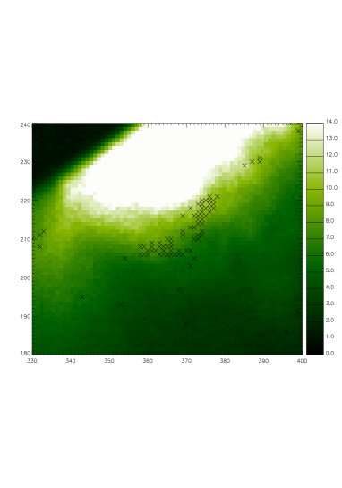
Figure 4: The area outside AR 9513 where the intensity oscillations with periodicity of 7-8$s$ were detected. All pixels with intensity oscillations are marked with ‘x’.

Figure 4 presents an area of the lower corona close to AR 9513 as observed by SECIS. Pixels with intensity oscillations that passes the established criteria are marked with ‘x’. The detections included in this Figure are, in their majority, due to plasma intensity oscillation in the solar corona and not due to atmospheric or instrumental effects for mainly two reasons:

1. The spatial distribution of the detected oscillations, unlike that of Figures 2 and 3, is not random, but highly concentrated in one area.

2. All 66 detections of interest are gathered in a very compact area. Figure 5 contains all oscillations in a 25$\times$19 pixels frame of 475 pixels in total. Based on the previous statistics an area of the moon or outer corona of the same size should have 2.4 detections due to atmospheric or instrumental effects.

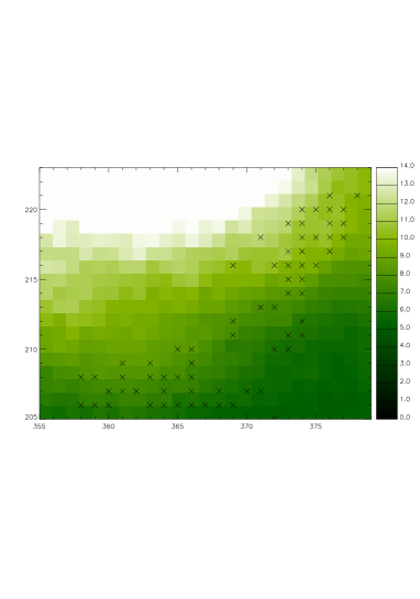
Figure 5: The area of AR 9513 with the highest population of oscillations with 7-8$s$ periodicity. This area is 25$\times$19 pixels in size (475 pixels in total). Based on the statistics calculated by the sample Moon and upper corona areas (see Figures 2 and 3), on average, there should be 2.4 detections due to atmospheric or instrumental effects.

Figure 6: Wavelet analysis of pixel x=374, y=211. This is a typical sample of a detection of intensity oscillations in the area of Figure 5. The rest of the detections seen on Figure 1 and this image do not pass the criteria established by [13].

Figure 1 is a display the wavelet analysis of the example point x=374, y=211 while Figure 6 is a zoom-in of the area of Figure 1 that contains the oscillations that pass the criteria established by [13].

Figure 6 has an interesting feature that appears in some of the 66 detections reported here and has not been seen in the 1999 observations yet. Although not detected by the automated software, as it does not satisfy the duration criteria established by [13], there is an oscillation contemporary to the main detection at exactly half the periodicity. This detection lasts for $\sim$12$s$ and starts almost simultaneously with the main oscillation, 7.5 $s$. As this secondary oscillation does not satisfy the duration criteria of [13], we would normally ignore it, but there is a number of coincidences that make it worth reporting. Namely, the oscillation starts practically simultaneously with the main one (and definitely within the limits of the mother wavelet time resolution) and it has exactly half of the periodicity of the main detection. Those two properties make it a perfect candidate for identification as a second order sausage-mode oscillation.

References

1. Hollweg, J.V., 1981, SolPhys, 70, 25

2. Parker, E.N., 1988, ApJ, 330, 474

3. Priest, E.R., Schrijver, C.J., 1999, SolPhys, 190, 1

4. Roberts B., Edwin P.M., Benz A.O., 1984, ApJ, 279, 857

5. Nakariakov V.M., Arber T.D., Ault C.E., Katsiyannis A.C., Williams D.R., 2004, MNRAS, 349, 705

6. Koutchmy, S., Žugžda, Y.D. & Locǎns, V., 1983, A&A, 120, 185

7. Pasachoff, J.M. & Landman, D.A., 1984, Sol. Phys., 90, 325

8. Singh, J., Cowsik, R., Raveendran, A.V., Bagare, S.P., Saxena, A. K., Sundararaman, K., Krishan, V., Naidu, N., Samson, J.P.A., Gabriel, F., 1997, Sol. Phys., 170, 235

9. Cowsik, R., Singh, J., Saxena, A.K., Srinivasan, R. & Raveendran, A.V., 1999, Sol. Phys., 188, 89

10. Pasachoff, J.M., Badcock, B.A., Russell, K.D. & Sea ton, D.B., 2002, Sol. Phys., 207, 241

11. Williams, D.R., Phillips, K.J.H., Rudawy P., Mathioudakis, M., Gallagher, P. T., O’Shea, E., Keenan, F. P., Read, P., Rompolt, B., 2001, MNRAS, 326, 428

12. Williams, D. R., Mathioudakis, M., Gallagher P.T., Phillips, K. J. H., McAteer, R. T. J., Keenan, F. P., Rudawy, P., Katsiyannis, A. C., 2002, MNRAS, 336, 747

13. Katsiyannis, A. C., Williams, D. R., McAteer, R. T. J., Gallagher, P. T., Keenan, F. P., Murtagh, F., 2003, A&A, 406, 709

14. Phillips, K.J.H., Read, P., Gallagher P.T., Keenan, F. P., Rudawy, P., Rompolt, B., Berlicki, A., Buczylko, A., Diego, F., Barnsley, R.,Smartt, R.N., Pasachoff, J.M., Badcock, B.A., 2000, Sol. Phys., 193, 259

15. Katsiyannis, A. C., McAteer, R. T. J., Williams, D. R., Gallagher, P. T., Keenan, F. P., 2004, SoHO, 13, 459

16. Torrence & C., Compo, G.P., 1998, Bull. Amer. Meteor. Soc., 79, 61