Physics of accretion in the millisecond pulsar XTE J1751–305

Abstract

We have undertaken an extensive study of X-ray data from the accreting millisecond pulsar XTE J1751–305 observed by RXTE and XMM-Newton during its 2002 outburst. In all aspects this source is similar to a prototypical millisecond pulsar SAX J1808.4–3658, except for the higher peak luminosity of 13 per cent of Eddington, and the optical depth of the hard X-ray source larger by factor $\sim$2. Its broad-band X-ray spectrum can be modelled by three components. We interpret the two soft components as thermal emission from a colder ($kT\sim 0.6$ keV) accretion disc and a hotter ($\sim 1$ keV) spot on the neutron star surface. We interpret the hard component as thermal Comptonization in plasma of temperature $\sim$40 keV and optical depth of $\sim$1.5 in a slab geometry. The plasma is heated by the accretion shock as the material collimated by the magnetic field impacts on to the surface. The seed photons for Comptonization are provided by the hotspot, not by the disc. The Compton reflection is weak and the disc is probably truncated into an optically thin flow above the magnetospheric radius. Rotation of the emission region with the star creates an almost sinusoidal pulse profile with rms amplitude of 3.3 per cent. The energy-dependent soft phase lags can be modelled by two pulsating components shifted in phase, which is naturally explained by a different character of emission of the optically thick spot and optically thin shock combined with the action of the Doppler boosting. The observed variability amplitude constrains the hotspot to lie within 3–4$\degr$ of the rotational pole. We estimate the inner radius of the optically thick accreting disc of about 40 km. In that case, the absence of the emission from the antipodal spot, which can be blocked by the accretion disc, gives the inclination of the system to be $\gtrsim 70\degr$.

1 Introduction

Millisecond radio pulsars are believed to be spun-up to their fast rotational speeds during the phase of accretion from their companion stars (for a review see e.g. Bhattacharya 1995). Though fast radio pulsars have been known for over 20 years, accretion-powered millisecond pulsars had proven to be an elusive missing link for a long time. SAX J1808.4–3658, the first millisecond pulsar (spin period $P_{s}$ = 2.5 ms) in a low-mass X-ray binary (LXMB) was discovered in 1998 (Wijnands & van der Klis, 1998a) by Rossi X-ray Timing Explorer (RXTE). Recent discoveries of XTE J1751–305 ($P_{s}$ = 2.3 ms; Markwardt et al. 2002, hereafter M02), XTE J0902–314 ($P_{s}$ = 5.4 ms; Galloway et al. 2002), XTE J1807–294 ($P_{s}$ = 5.3 ms; Markwardt, Smith & Swank 2003), XTE J1814–338 ($P_{s}$ = 3.2 ms; Markwardt & Swank 2003), and IGR J00291+5934 ($P_{s}$ = 1.67 ms; Eckert et al. 2004; Markwardt et al. 2004) have brought the total number of currently known accreting millisecond pulsars to six.

Gierliński, Done & Barret (2002, henceforth GDB02) analysed energy spectra of SAX J1808.4–3658 from the 1998 outburst. The X-ray spectral shape remained almost constant throughout the outburst and could be fitted by a blackbody and thermal Comptonization. Weak Compton reflection ($\Omega/2\pi\sim 0.1$) was also detected. GDB02 interpreted the blackbody as emission from the heated spot on the neutron star, and the Comptonization taking place in an accretion column, as the material collimated by the magnetic field impacts on to the neutron star surface. The phase-resolved X-ray spectra showed that pulsation of these two components is shifted in phase. Poutanen & Gierliński (2003, henceforth PG03) applied the full relativistic treatment to the energy-resolved pulse profiles of SAX J1808.4–3658 and studied the effects of different angular distribution of the emission pattern from the blackbody and Comptonization components. They estimated the neutron star radius to be $\sim$ 6.5 and $\sim$ 11 km for a 1.2 and 1.6 M_⊙ neutron star, respectively.

XTE J1751–305 is in a very tight binary, with the orbital period of only 42 minutes and the mass function of the pulsar $1.3\times 10^{-6}$ M_⊙, which gives a minimum mass for the companion of about 0.014 M_⊙ (M02). The distance, $D$, to the source is not known, though as it might be related to the Galactic centre, therefore we assume $D\sim$ 8.5 kpc. M02 estimated the distance to be greater than 7 kpc, using indirect arguments.

In this paper we examine the X-ray spectra of XTE J1751–305 from its April 2002 outburst, observed by XMM-Newton and RXTE. In Section 4 we study the (phase-averaged) energy spectra, in particular the broad-band 0.7–200 keV simultaneous spectrum from both instruments. We model them by the blackbody and Comptonization from hotspot and accretion shock, respectively. We also show that another soft component, from the accretion disc, is required. In Sections 5 and 6 we study phase-resolved spectra and interpret them in terms of two independently pulsating spectral components. In Section 8 we discuss our results and derive constraints on the accretion flow geometry which occur to be very similar to those found for SAX J1808.4–3658 (GDB02).

2 Observations

2.1 RXTE

RXTE observed XTE J1751–305 from 3^rd to 30^th of April 2002. We reduced these data using ftools version 5.3. Proportional Counter Array (PCA) units 1 and 4 were switched off for most of this period. As unit 0 lost its propane layer in May 2000 and its calibration is uncertain, we decided to use the data from units 2 and 3 only. For each of the observations with the unique identifier (obsid) we extracted energy spectra in 3–20 keV band. Analogous Crab spectra from the same period show features at a level of  1 per cent, most likely of the instrumental origin. Therefore, we applied 1 per cent systematic errors in each of the PCA energy channels in addition to statistical errors.

In addition to the PCA data we also extracted 20–200 keV High-Energy X-ray Timing Experiment (HEXTE) spectra from both detector clusters. During observation of April 3 HEXTE did not perform ‘rocking’ and did not record background, so we could not use these data. Table 1 contains log of the RXTE observations analysed in this paper.

XTE J1751–305 is only  2^∘ away from the Galactic centre, so its X-ray spectrum is contaminated by the diffuse Galactic ridge emission. Fortunately, RXTE performed several observations in the direction of XTE J1751–305 after the outburst (see fig. 1 in M02). Between 20^th and 25^th of April PCA count rate remained constant and minimal (there was a small outburst later on), indicating its origin from the background. We accumulated average PCA spectrum from this period (with average count rate of $12.01\pm 0.04$ s^-1 in detectors 2+3, all layers) and used it as an additional background for outburst observations. Table 1 contains PCA count rates corrected for this effect. HEXTE spectra were not affected by the diffuse emission.

We extracted phase-resolved energy spectra from the PCA Event mode files (configuration E_125us_64M_0_1s) with timing resolution of 122 $\mu$s (except for the April 3 observation where we used GoodXenon mode files, with resolution of 1 $\mu$s). We generated folded light-curves in 16 phase bins, for each PCA channel, using events from all layers of units 2 and 3. We have chosen beginning of the phase ($\phi=0$) at the bin with lowest 3–20 keV count rate. Photon arrival times were corrected for orbital movements of the pulsar and the spacecraft, using ephemeris from M02. Background files were created from standard models, with addition of the April 20–25 spectrum to represent the diffused emission. We also extracted power density spectra (PDS) from the same event data files, but using units 0, 2 and 3. We have created power density spectra in the ${}^{1}/_{128}$–512 Hz frequency range from averaging fast Fourier transforms over 128-s data intervals.

2.2 XMM-Newton

XMM-Newton observed XTE J1751–305 on 2002 April 7, with the total exposure of 33 ks. We reduced the data from European Photo Imaging Camera PN (EPIC-pn) detector using sas version 5.4.1. and following guidelines in the MPE cookbook (http://wave.xray.mpe.mpg.de/xmm/cookbook). The detector operated in timing mode where spatial information was compressed into one dimension. We extracted EPIC-pn spectrum from a stripe in raw CCD coordinates RAWX (36,56), collecting single and double events only. The background was extracted from the adjacent stripe in RAWX (16,36).

All spectral analysis (both phase-resolved and phase-averaged) was done using the xspec 11.2 spectral package (Arnaud, 1996). The error of each model parameter is given for a 90 per cent confidence interval, except for the pulse profiles in Sec. 6, where we used 1$\sigma$ errors. The relative normalization of the PCA and HEXTE instruments is uncertain, so we allowed this to be an addition free parameter in all spectral fits.

Table 1: Log of RXTE observations analysed in this paper. Start and end times are in the UT days of April 2002. Exposures are in seconds and (background subtracted) count rates are in counts per second from detectors 2 and 3 of PCA and separately from cluster 0 and 1 of HEXTE. During the first observation HEXTE did not observe background.

				PCA (2+3)		HEXTE 0		HEXTE 1
No.	Obsid	Start	End	Exposure	Count rate	Exposure	Count rate	Exposure	Count rate
1	70134-03-01-00	3.653	3.720	3168	250.5$\pm$0.6	N/A		N/A
2	70131-01-01-00	4.644	4.912	10960	237.3$\pm$0.5	3520	18.7$\pm$0.2	3461	15.2$\pm$0.2
3	70134-03-02-00	5.162	5.179	720	226.5$\pm$0.8	257	19.8$\pm$0.9	263	14.4$\pm$0.8
4	70131-01-02-00	5.535	5.773	6384	214.8$\pm$0.5	2039	17.3$\pm$0.3	2012	14.0$\pm$0.2
5	70131-01-03-01	6.525	6.542	1456	190.0$\pm$0.6	425	16.4$\pm$0.6	431	12.3$\pm$0.5
6	70131-01-03-00	6.591	6.763	9200	185.9$\pm$0.4	2859	15.3$\pm$0.2	2791	12.0$\pm$0.2
7	70131-01-04-00	7.515	7.753	12416	163.3$\pm$0.4	3839	13.7$\pm$0.2	3809	10.7$\pm$0.2
8	70131-01-05-03	8.061	8.083	1168	162.4$\pm$0.6	432	14.3$\pm$0.7	410	8.9$\pm$0.6
9	70131-01-05-02	8.131	8.149	864	154.8$\pm$0.7	313	14.4$\pm$0.9	302	10.3$\pm$0.8
10	70131-01-05-01	8.199	8.215	576	155.4$\pm$0.8	204	12.6$\pm$1.1	198	9.3$\pm$1.0
11	70131-01-05-04	8.267	8.467	2368	147.7$\pm$0.5	754	13.8$\pm$0.5	749	9.4$\pm$0.4
12	70131-01-05-000	8.505	8.743	12544	144.9$\pm$0.4	3897	13.4$\pm$0.2	3799	9.6$\pm$0.2
13	70131-01-05-00	8.772	9.007	4752	143.1$\pm$0.4	1645	12.9$\pm$0.3	1586	8.9$\pm$0.2
14	70131-01-06-00	9.435	9.601	8800	129.0$\pm$0.3	2831	12.6$\pm$0.2	2731	8.6$\pm$0.2
15	70131-01-06-01	9.627	9.799	8464	126.1$\pm$0.3	2714	12.1$\pm$0.2	2660	8.0$\pm$0.2
16	70131-01-07-00	10.418	10.525	6592	112.1$\pm$0.3	2093	10.4$\pm$0.3	2092	7.1$\pm$0.2
17	70131-01-07-01	10.551	10.789	11552	108.6$\pm$0.3	3619	9.9$\pm$0.2	3573	6.8$\pm$0.2
18	70131-01-08-000	11.409	11.713	15552	94.3$\pm$0.3	4840	8.9$\pm$0.2	4794	5.9$\pm$0.1
19	70131-01-08-00	11.742	11.912	6704	91.2$\pm$0.3	2376	8.7$\pm$0.2	2334	5.5$\pm$0.2
20	70131-01-09-000	12.333	12.638	9632	56.7$\pm$0.2	2934	5.9$\pm$0.2	2870	3.3$\pm$0.2
21	70131-01-10-00G	13.322	13.496	5120	13.7$\pm$0.2	1683	1.3$\pm$0.3	1686	0.6$\pm$0.2

3 Outburst

Figure 1: 3–20 keV unabsorbed flux of observations 1–21 (Table 1). The solid lines correspond to $F\propto e^{-t/7.2^{\rm d}}$ and $F\propto e^{-t/0.63^{\rm d}}$.

Fig. 1 shows the evolution of the 3–20 keV unabsorbed flux during the outburst (see also M02). The peak flux during observation 2 was $1.5\times 10^{-9}$ erg s^-1 cm^-2. Using a Comptonization model (see Section 4), we estimated the peak bolometric X-ray/$\gamma$-ray flux of $3.1\times 10^{-9}$ erg s^-1 cm^-2. For a distance of 8.5 kpc (assuming the source to be close to the Galactic centre) this corresponds to the bolometric luminosity of $2.7\times 10^{37}$ erg s^-1, or 13 per cent of Eddington luminosity $L_{\rm Edd}$ for a 1.4 M_⊙ neutron star. This is much brighter than SAX J1808.4–3658 with the estimated peak bolometric luminosity of 2.2 per cent of $L_{\rm Edd}$ (GDB02).

The light curve of XTE J1751–305 shows a striking similarity to that of SAX J1808.4–3658 (see fig. 1 in Gilfanov et al. 1998; see also M02). After the peak the flux declined exponentially, with $e$-folding factor of 7.2 days (10 days in SAX J1808.4–3658), until it reached a break after which the flux dropped suddenly with the $e$-folding factor of $\sim$0.6 days (1.3 days in SAX J1808.4–3658). The break in the light curve is most likely associated with the onset of the cooling wave in the accretion disc (GDB02).

4 Phase-averaged energy spectra

Table 2: Summary of spectral models used in this paper.

Model	xspec components	Description
DTH	wabs*(diskbb+thcomp)	Multicolour disc and thermal Comptonization of the disc photons.
DTF	wabs*(diskbb+thcomp)	The same as DTH, but the seed photon temperature is free and independent of the disc.
DBTH	wabs*(diskbb+bbodyrad+thcomp)	Multicolour disc, single-temperature blackbody and thermal Comptonization of the blackbody photons.
DBTF	wabs*(diskbb+bbodyrad+thcomp)	The same as DBTH, but the seed photon temperature is free and independent of the blackbody.
DBPS	wabs*(diskbb+bbodyrad+compps)	The same as DBTH, with thcomp replaced by compps.
DBPF	wabs*(diskbb+bbodyrad+compps)	The same as DBTF, with thcomp replaced by compps.

4.1 Physical picture and spectral models

If the neutron star magnetic field is strong enough, the accreting material will follow magnetic field lines and form a shock close to the neutron star surface (for the accretion geometry see fig. 12 of GDB02 and Romanova et al., 2004). The shock is pinned down to the stellar surface at luminosity of a few per cent of $L_{\rm Edd}$ (Basko & Sunyaev, 1976; Lyubarskii & Sunyaev, 1982). Gravitational energy is dissipated in the shock and is transferred from the protons to the electrons by Coulomb collisions. The main cooling mechanism is Comptonization of soft photons provided by the neutron star. The stellar surface is heated under the shock, while the hard X-rays, produced in the shock, can also irradiate the surrounding surface, so that the black body emission region can cover a somewhat larger area.

Such a physical picture is in agreement with observations of SAX J1808.4–3658 (GDB02, PG03). We presume that XTE J1751–305 is a similar source to SAX J1808.4–3658. Thus we expect emission from the hotspot on the neutron star surface, which we model as a blackbody. We also expect emission from the accretion shock, which we model by thermal Comptonization. We consider two possible geometries of the shock and hotspot, shown in Fig. 2. For the phase-averaged fits we assume that the angle between the rotation axis and the magnetic pole is small, so that the slab model of the shocked region viewed at a fixed angle is justified. We will show later in Sec. 8.3.4 that this assumption is feasible. In addition to the above components we might expect thermal emission from the accretion disc and Compton reflection from the disc and/or neutron star surface.

For the spectral description we use the models summarized in Table 2. Their spectral components are as follows. bbodyrad is a single-temperature blackbody, normalized to its apparent area (at a given distance), which represents the emission from a hotspot at a neutron star surface. diskbb is a multicolour (accretion) disc model (Mitsuda et al., 1984), normalized to the inner disc radius (at a given distance). We correct the inner disc radius for the spectral hardening with factor $f_{\rm col}$ = 1.8 (Shimura & Takahara, 1995) and for the torque-free inner boundary condition, with factor $\zeta$ = 0.37 (Gierliński et al., 1999): $R_{\rm in}=f^{2}_{\rm col}\zeta R_{\rm in,apparent}$. The exact value of the hardening factor is not well known, but recent numerical accretion disc simulations place it between 1.8 and 2.0, increasing with luminosity (Davis et al. 2004). Additional uncertainty comes from general and special relativistic corrections (see e.g. Cunningham, 1975; Zhang, Cui & Cheng, 1997). Later in this paper we discuss the effects of the disc with the continuous torque through the inner radius.

thcomp is a thermal Comptonization model, using an approximate solution of the Kompaneets (1956) equation (Zdziarski, Johnson & Magdziarz, 1996). It is parameterized by the asymptotic power-law photon index, $\Gamma$, electron temperature, $T_{\rm e}$ and seed photon temperature, $T_{\rm seed}$. compps is another Comptonization model (Poutanen & Svensson, 1996). It finds an exact numerical solution of the Comptonization problem explicitly considering successive scattering orders. It also allows for various hot plasma geometries. For a slab geometry of the emission region, this model is parameterized by the optical depth of the scattering medium, $\tau$, electron temperature, $T_{\rm e}$, seed photon temperature, $T_{\rm seed}$, and the inclination angle to the slab normal. The interstellar absorption was described by model wabs with the hydrogen column density $N_{\rm H}$ as a parameter.

4.2 XMM-Newton

Miller et al. (2003) successfully fitted EPIC-pn spectrum of XTE J1751–305 with a simple phenomenological model of a blackbody and power law. We confirmed that this model gave a very good reduced $\chi^{2}/\nu$ = 2013/1859, indeed. There are, however, two fundamental issues here. Firstly, the most probable radiative process that gives rise to emission above $\sim$1 keV is thermal Comptonization which can be described by a power law in a narrow energy band only. At energies around seed photon temperature, the Comptonization spectrum has a low-energy cutoff. Secondly, the best-fitting spectral index of the power law ($\Gamma=1.44\pm 0.01$) is in strong disagreement with RXTE data, where the spectrum is much softer, $\Gamma\sim$ 1.8–1.9 (see below).

Therefore, we tried a physically motivated model. Instead of the power law we used thcomp, assuming that the seed photons were from the blackbody component. This model gave rather poor fit with $\chi^{2}/\nu$ = 2754/1859 and broad residuals implying wrong shape of the continuum. In the second attempt we allowed the seed photons for Comptonization to be independent of the blackbody component. This fit was much better ($\chi^{2}/\nu$ = 2044/1858), but the large apparent area of the blackbody, $A_{\rm bb}\sim$ 1400 ($D$/8.5 kpc)² km², ruled out its origin from the neutron star surface. Instead, it rather originated from the accretion disc, so we replaced the blackbody by the multicolour disc (model DTF in Table 2). The results are shown in Table 3. The seed photons for Comptonization ($kT_{\rm seed}=0.68_{-0.01}^{+0.02}$ keV) were much hotter than the disc photons ($kT_{\rm disc}=0.38_{-0.02}^{+0.03}$ keV) and they might have originated from the neutron star surface (see Gierliński & Done 2002; GDB02). We tried to model the surface emission by adding a single-temperature blackbody component with its temperature tied to the seed photons (see Fig. 2a). Model DBTH improved the fit by $\Delta\chi^{2}=28$ over model DTF, with one degree of freedom less (Table 3). The apparent area of this blackbody, $A_{\rm bb}=36_{-4}^{+3}$ ($D$/8.5 kpc)² km², was consistent with a hotspot on the neutron star surface.

Table 3: Best-fitting parameters of the models applied to EPIC-pn data. Models are described in Table 2. Inner disc radius $R_{\rm in}$ and apparent area of the blackbody $A_{\rm bb}$ were calculated assuming distance of 8.5 kpc. thcomp temperature was fixed at 30 keV.

Model	DTF	DBTH
$N_{\rm H}$ (1022 cm-2)	1.04${}_{-0.03}^{+0.02}$	1.01${}_{-0.02}^{+0.01}$
$kT_{\rm disc}$ (keV)	0.38${}_{-0.02}^{+0.03}$	0.51${}_{-0.03}^{+0.09}$
$R_{\rm in}\sqrt{\cos i}$ (km)	16.5${}_{-2.6}^{+2.5}$	10.0${}_{-2.2}^{+1.5}$
$kT_{\rm bb}$ (keV)	-	0.89${}_{-0.05}^{+0.09}$
$A_{\rm bb}$ (km2)	-	36${}_{-4}^{+3}$
$\Gamma$	1.90${}_{-0.01}^{+0.02}$	1.72${}_{-0.14}^{+0.07}$
$kT_{\rm seed}$ (keV)	0.68${}_{-0.01}^{+0.02}$	$=kT_{\rm bb}$
$\chi^{2}/\nu$	2039.5/1858	2011.9/1857

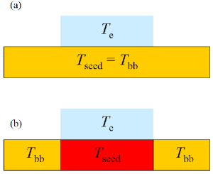
Figure 2: Schematic geometries of the emission region, consisting of the accretion shock above, and the hotspot on the surface of the neutron star. (a) Geometry corresponds to a small temperature gradient in the hotspot, i.e. the case where seed photons have the same temperature as the photons in the observed black body component (models DBTH, DBPS). (b) Geometry corresponds to a large temperature gradient where seed photons are hotter than the illuminated region of the neutron star surface around the shock, which gives rise to the observed black body emission (models DBTF, DBPF). The emitting region corresponds to a point where the accretion column impacts on the surface (see fig. 12 in GDB02).

There were no distinct features around 7 keV in the residuals, and we did not detect Compton reflection at a statistically significant level in the EPIC-pn spectrum. The best-fitting amplitude of reflection was only $\Omega/2\pi=0.01_{-0.01}^{+0.06}$ giving fit improvement of $\Delta\chi^{2}$ = 1.9 with two degrees of freedom less.

4.3 Simultaneous XMM-Newton and RXTE

Figure 3: EPIC-pn/PCA cross-calibration. The figure shows the residuals (data-to-model ratio) of the EPIC-pn (triangles) and PCA (squares) spectra to a power-law model. The EPIC-pn spectrum was rebinned for presentation only.

Encouraged by the results from XMM-Newton we extended the observed bandwidth by adding an RXTE spectrum. Observation 6 from Table 1 was simultaneous with EPIC-pn data. It overlapped with a small fraction of the EPIC-pn exposure only, but there was very little spectral variability throughout this observation, so spectra from both instruments should be the same. We also checked the cross-calibration between the two instruments to look for possible response discrepancies. We fitted both spectra in the overlapping 3–10 keV band by a power law. The spectral indices were in good agreement, $\Gamma=1.660\pm 0.005$ and $1.667\pm 0.015$ for EPIC-pn and PCA, respectively. The residuals were also quite similar (see Fig. 3), indicating nearly identical spectral shape. We decided that the broad-band analysis of the simultaneous XMM-Newton and RXTE was feasible. We fitted the EPIC-pn spectrum and PCA/HEXTE observation 6 together with a sequence of models, which are summarized in Table 2. We allowed for the relative normalization of these instruments to be free and used PCA normalization for flux calculations. The relative normalizations of EPIC-pn, HEXTE clusters 0 and 1 with respect to PCA were 0.64, 0.57 and 0.74, respectively, for our best fit. The fit results are shown in Table 4 and two of the fitted spectra in Fig. 4.

Figure 4: Broad-band spectrum of XTE J1751–305 from EPIC-pn, PCA and HEXTE. The models consists of the multicolour disc (green curve), single-temperature blackbody (blue curve), and thermal Comptonization of the blackbody photons (magenta curve). The dotted curves show unabsorbed spectral components. Panel (a) shows model DBTH, corresponding to the shock geometry shown in Fig. 2a. Panel (b) shows model DBTF, with geometry as in Fig. 2b. See Table 2 for model description and Table 4 for best fitting parameters. The lower panels shows the residuals of EPIC-pn (cyan), PCA (black) and HEXTE (blue).

Table 4: Best-fitting parameters of several models applied to EPIC-pn/PCA/HEXTE simultaneous data. The models are summarized in Table 2. Inner disc radius $R_{\rm in}$ and apparent area of the blackbody $A_{\rm bb}$ are calculated assuming distance of 8.5 kpc. The spectrum and components of the model DBTH are shown in Fig. 4.

Model	DTH	DTF	DBTH	DBTF	DBPS	DBPF
$N_{\rm H}$ (1022 cm-2)	0.926${}_{-0.004}^{+0.005}$	1.050${}_{-0.019}^{+0.033}$	1.015${}_{-0.015}^{+0.020}$	1.000${}_{-0.011}^{+0.023}$	1.012${}_{-0.017}^{+0.018}$	0.998${}_{-0.013}^{+0.014}$
$kT_{\rm disc}$ (keV)	1.13$\pm$0.04	0.35$\pm 0.02$	0.46$\pm 0.03$	0.58$\pm$0.04	0.48$\pm$0.04	0.61$\pm$0.05
$R_{\rm in}\sqrt{\cos i}$ (km)	3.6$\pm$0.2	25.2${}_{-2.7}^{+5.7}$	14.9${}_{-1.9}^{+2.7}$	10.4${}_{-1.1}^{+1.8}$	14.0$\pm$2.0	9.8${}_{-1.2}^{+1.7}$
$kT_{\rm bb}$ (keV)	-	-	0.81$\pm 0.03$	0.95$\pm$0.04	0.84$\pm$0.03	1.00$\pm$0.05
$A_{\rm bb}$ (km2)	-	-	$49\pm 4$	95${}_{-9}^{+14}$	39${}_{-5}^{+11}$	91${}_{-12}^{+16}$
$\Gamma$	1.78$\pm$0.01	1.86$\pm 0.01$	1.81$\pm 0.01$	1.94$\pm$0.05	-	-
$\tau$	-	-	-	-	1.93${}_{-0.15}^{+0.23}$	1.47${}_{-0.14}^{+0.26}$
$kT_{\rm e}$ (keV)	22${}_{-2}^{+3}$	32${}_{-5}^{+8}$	$25_{-3}^{+4}$	42${}_{-10}^{+70}$	29$\pm$4	36${}_{-5}^{+3}$
$kT_{\rm seed}$ (keV)	= $kT_{\rm disc}$	0.64$\pm$0.01	= $kT_{\rm bb}$	1.75$\pm$0.18	=$kT_{\rm bb}$	2.2${}_{-0.3}^{+0.1}$
$A_{\rm seed}$ (km2)	-	-	-	-	790${}_{-140}^{+50}$	20${}_{-7}^{+17}$
$\chi^{2}/\nu$	2271.8/1984	2208.1/1983	2154.3/1982	2127.0/1981	2141.2/1982	2125.5/1981

First, we tested the possibility that the seed photons for Comptonization came from the accretion disc (model DTH). The model fitted the data fairly well (reduced $\chi^{2}/\nu=1.15$). It required however a very small inner radius of the disc, $R_{\rm in}\sqrt{\cos i}=3.6\pm 0.2$ ($D$/8.5 kpc) km (here $i$ is the disc inclination angle), smaller than the expected neutron star radius.

The model DTF, where the seed photons for Comptonization were independent of the disc temperature, gave a good fit to the EPIC-pn data in Section 4.2. We applied the same model to the broad-band spectrum (with free $T_{\rm e}$). It improved the fit by $\Delta\chi^{2}=63.7$ (at 1983 d.o.f.) with respect to DTH. The disc temperature was much lower and its inner disc radius much larger, making it consistent with an overall picture of a millisecond accreting pulsar (GDB02) or, more generally, an atoll source in the island state (e.g. Barret, 2001).

Adding the blackbody source of the seed photons (presumably neutron star surface) as an explicit component (model DBTH) improved the fit further by $\Delta\chi^{2}=53.8$ (at 1982 d.o.f.). The apparent area of the blackbody component, $A_{\rm bb}=49\pm 4$ ($D$/8.5 kpc)² km², was consistent with a hotspot on the neutron star surface. However, this component did not produce enough photons for Comptonization. The Comptonization spectrum of $\Gamma\sim 1.8$ and $kT_{\rm e}\sim 25$ keV requires a similar luminosity in the seed and Comptonized photons, while the observed blackbody component was $\sim$ 30 times weaker than thcomp. This means that majority of the seed photons were not visible, e.g. because they were covered by the Comptonizing accretion column (Fig. 2b). In fact, spectral fits with compps (see below) showed that the actual area of the seed photons source greatly exceeded the expected area of the neutron star.

Therefore, we considered one more model (DBTF), which included the disc emission, the blackbody and Comptonization of unseen seed photons of much higher temperature (see Fig. 2b). This model produced a very good fit, improving previous results by $\Delta\chi^{2}$ = 27.3. It gave high seed photon temperature of $kT_{\rm seed}=1.75\pm 0.18$ keV and much softer spectral index of $\Gamma=1.94\pm 0.05$. As we show below in this section, the seed photons in this model were consistent with the hotspot on the neutron star.

Next, we tested how sensitive the above results were to the choice of a particular model. We replaced thcomp by another Comptonization code, compps. It computes the exact numerical solution of the radiative transfer equation for Comptonization in a given geometry and allows finding the normalization (or apparent area) of the blackbody seed photons. We chose a geometry in which a slab of hot plasma is irradiated from below by the blackbody seed photons. The parameter $\tau$ in the model is the vertical optical depth of the slab, so the actual line-of-sight optical depth depends on the inclination angle $i$. Unlike thcomp, the unscattered seed photons transmitted through the slab are already included in compps model, so any additional blackbody component in the model corresponds to photons not entering the hot plasma. This geometry is consistent with an accretion shock above the hotspot on the neutron star surface (GDB02; PG03).

For this model we assumed that the inclination angle of the slab with respect to the observer was equal to the inclination of the system, $i=60^{\circ}$. This is, certainly, an approximation, as the accretion shock rotates with the neutron star surface. However, as we show later in this paper (see Section 8.3 and Fig. 15) the magnetic inclination $\theta$ is small, $\la$ 10^∘, so the angle at which we see the shock doesn’t vary much.

In the model DBPS, corresponding to the geometry in Fig. 2(a), the temperature of the seed photons was tied to the blackbody component. The apparent area of the source of the seed photons was very large, $A_{\rm seed}=790_{-140}^{+50}$ ($D$/8.5 kpc)² km². This definitely could not be a hotspot on the surface, unless the distance to the source is less than $\sim$3 kpc (but see Section 8.4).

A fit with seed photons independent of the blackbody temperature (model DBPF corresponding to a geometry in Fig. 2b) gave better $\chi^{2}$, but more importantly, yielded much smaller apparent area of the seed photons of $20_{-7}^{+17}$ ($D$/8.5 kpc)² km². On the other hand, the apparent area of the (independent) blackbody component was significantly larger, $A_{\rm bb}\approx 90$ ($D$/8.5 kpc)² km².

The great advantage of compps model is that it computes angle-dependent spectrum. For an intermediate optical depth of the slab of $\tau\sim$ 1.5–2.0 the overall spectral shape of the Comptonized continuum depends only weakly on the observer’s angle with respect to the slab. The main effect is the amount of unscattered seed photons seen at different angles, as it is very sensitive to the actual optical depth along the line of sight, $\tau/\cos i$. So far, we have assumed quite large inclination angle of 60^∘. To check the angular dependence we repeated the fits with models DBPS and DBPF at 30^∘. The DBPS fit was dramatically worse by $\Delta\chi^{2}$ = 75.4. Smaller angle gave larger, not consistent with the observed spectrum, amount of unscattered seed photons. The DBPF fit, with more freedom of shaping the low-energy part of the spectrum gave the fits worse by $\Delta\chi^{2}$ = 7.1 and optical depth of $\tau=2.54\pm 0.15$, larger than at 60^∘ by expected factor of $\cos 30^{\circ}/\cos 60^{\circ}$. The actual line-of-sight optical depth to the seed photons was about 2.9, so the observed unscattered fraction of the seed photons was about 5 per cent. This explains why thcomp, with no unscattered blackbody photons included in the model, could fit the data well. When inclination was allowed to be free, the best-fitting values were $i=79_{-35}^{+11}$ and $65_{-19}^{+10}$ deg, for DBPS and DBPF, respectively.

No reflection was significantly detected in any of these models. We found only upper limits on $\Omega/2\pi$ of 0.06 and 0.41, from DBTF and DBPF, respectively. The first model incorporated reflection with a self-consistent iron line (Życki, Done & Smith, 1998), while the second one included an independent diskline model, with one more free parameter and a less strict constrain.

Figure 5: Fitting results of the blackbody plus thermal Comptonization model (DBTF from Table 2, without disc component) to the outburst RXTE spectra. The electron temperature was fixed at 42 keV, the absorption column at $1.0\times 10^{22}$ cm^-2. $\Gamma$ is the asymptotic photon spectral index, $kT_{\rm seed}$ (keV) is the seed photon temperature, $N_{\rm hard}$ ($10^{-9}$ erg s^-1 cm^-2) is the normalization of the Comptonized component at 10 keV, $kT_{\rm soft}$ (keV) and $A_{\rm soft}$ (km²) are the temperature and apparent area of the soft (blackbody) component, respectively. The fraction of Eddington luminosity, $L_{\rm bol}/L_{\rm Edd}$, and $A_{\rm soft}$ are calculated for a distance of 8.5 kpc.

The total unabsorbed bolometric flux from model DBTF was $F_{\rm bol}=2.9\times 10^{-9}$ erg s^-1 cm^-2, which corresponds to luminosity $L_{\rm bol}=2.5\times 10^{37}$ erg s^-1 or $0.12L_{\rm Edd}$ for a 1.4 M_⊙ neutron star at a distance of 8.5 kpc. The contribution to the total luminosity from the disc and blackbody components was 9 and 13 per cent, respectively.

4.4 RXTE outburst

Finally, we analysed the RXTE spectra from Table 1 covering the whole outburst (observations 2–21). For spectral fitting we used some of the models from Table 2, however without the disc component, which could not be constrained by the PCA data and had little effect above 3 keV. We also fixed the absorption column at $N_{\rm H}=1.0\times 10^{22}$ cm^-2.

Model DBTH gave a good total (i.e. summed over all 20 observations) $\chi^{2}/\nu$ = 2153.7/2440. The spectral parameters remained roughly constant throughout the outburst. In this model the soft blackbody component was very weak, its normalization (or apparent area) consistent with zero in about half of the fits and its contribution to the bolometric luminosity negligible. On the other hand its temperature was well constrained, as it was equal to the temperature of the seed photons in the Comptonized component and constrained by the low-energy cutoff in the spectrum.

When we made seed photon temperature a free parameter (model DBTF), some of the fits become unstable, in particular the electron temperature was not constrained. We fixed $kT_{\rm e}$ = 42 keV (the value taken from the outburst average, see below). After this modification we obtain total $\chi^{2}/\nu$ = 2106.4/2240. The results are presented in Fig. 5. The blackbody and seed photon temperatures were slightly higher and the spectral index slightly softer in the beginning of the outburst, but apart from that the spectral shape remained amazingly constant throughout the outburst. The ratio of unabsorbed fluxes from Comptonization and blackbody was $\sim$ 6.

We also fitted the average spectrum of the entire outburst (co-added observations 2–21). Model DBTF gave a very good fit, $\chi^{2}/\nu=101.4/121$. The blackbody temperature was $kT_{\rm bb}=0.83\pm 0.06$, seed photon temperature $kT_{\rm seed}=1.46_{-0.18}^{+0.13}$ keV, the spectral index $\Gamma=1.93\pm 0.03$ and electron temperature $kT_{\rm e}=42_{-7}^{+9}$ keV. These parameters were consistent with those obtained from the combined XMM and RXTE fits. Compton reflection was not significantly detected again: the was only an upper limit on $\Omega/2\pi<0.15$, with fit improvement of $\Delta\chi^{2}$ = 2.0 and two degrees of freedom less. This average outburst spectrum formed a base for analysis of the phase-resolved spectra in Section 6.

4.5 Summary of spectral results

In the above section we have fitted the X-ray spectrum of XTE J1751–305 by models consisting of the emission from accretion disc, blackbody hotspot and optically thin Comptonization. We have considered two types of models, corresponding to hotspot/shock geometries sketched in Fig. 2. In the first geometry the seed photons for Comptonization originated from the hotspot (DBTH and DBPS, Fig. 4a). In the second geometry the seed photons were considerably hotter than the blackbody (DBTF and DBPF, Fig. 4b). The second geometry was preferred both from statistical point of view (it gave better fit) and from the physical constraints, as the first geometry required the area of the seed photons source larger than the neutron star surface. In the geometry of the short shock above the surface, GDB02 ruled out the origin of the seed photons from the accretion disc.

5 Pulse profiles

Fig. 6 shows the pulse profile of XTE J1751–305 accumulated over the entire outburst. It was not perfectly symmetric, a fit by a single sine function gave rather poor $\chi^{2}/\nu$ = 28.3/13. With the second harmonic added (its phase independent of the first one), the fit was much improved, $\chi^{2}/\nu$ = 17.3/11. The rms amplitudes, calculated from these fits, were 3.28$\pm$0.03 and 0.11$\pm$0.03 per cent for the first and second harmonic, respectively, which correspond to the peak-to-peak amplitudes $(F_{\max}-F_{\min})/(F_{\max}+F_{\min})$ of 4.6 and 0.15 per cent. The lower panel of Fig. 6 shows the residuals of the single-harmonic fit with the second harmonic function overplotted.

Figure 6: Pulse profile of XTE J1751–305. The upper panel shows the folded 2–60 keV PCA light curve accumulated over the entire outburst. The errors are of order of symbol size. The curve represents the model consisting of two harmonics. The lower panel shows the residuals of data minus first harmonic and the second harmonic model curve.

We investigated the energy dependence of the pulse profile. Fig. 7 shows the outburst-averaged pulse profile in three energy bands. The pulse amplitude decreased and its profile shifted towards earlier phase with increasing energy. This effect can be clearly seen in Fig. 8, where we calculated the amplitude and phase lag in each of the PCA energy channels by fitting their pulse profiles by a sine function. Fig. 8a shows the dependence of the pulse rms amplitude on energy, which decreased from around 3.3 per cent at 2–10 keV to less than 2.5 per cent at 20 keV. The absolute value of the time lag with respect to the energy channel 2–3.3 keV increased with energy up to about 120 $\mu$s at 10 keV, above which it seemingly saturated (Fig. 8b). The negative time lag means that the hard photons arrived earlier than the soft photons. This behaviour was very similar to other millisecond pulsars, SAX J1808.4–3658 (Cui, Morgan & Titarchuk 1998; GDB02), XTE J0929–314 (Galloway et al., 2002), and IGR J00291+5934 (Galloway et al., 2005).

Figure 7: Pulse profiles (outburst averaged) in three energy bands.

Figure 8: (a) The rms amplitude of the pulse profile as a function of energy. (b) Time lag of the pulse profile versus energy, with respect to the first energy channel, 2–3.3 keV.

Figure 9: Pulsation in the model consisting of the blackbody and Comptonization of the seed photons independent of this blackbody. Only normalizations of both components were free during the fits. This model with total $\chi^{2}/\nu$ = 501/688 is preferred over the pulsating index model from Fig. 10.

Figure 10: Pulsation in the model consisting of the blackbody and Comptonization of the seed photons independent of this blackbody. Only normalization of the hard component and its spectral index were free during the fits. This model gave worse fit, $\chi^{2}/\nu$ = 592/720, than the two pulsating components model from Fig. 9.

6 Phase-resolved energy spectra

The photon statistics in the phase-resolved spectra was very limited, as each of the phase bins contained only a sixteenth part of the total counts. This made spectral fitting of individual observations difficult. However, as we have shown in the previous section, the spectral shape remained almost constant throughout the outburst, so analysis of the outburst-averaged data was feasible. Thus, we fitted the average phase-resolved spectrum in each of the phase bins by the models developed earlier in this paper.

The best physically motivated models for the broad-band data were DBTF and DBPF, from which we chose DBTF as it is much faster to compute. We simplified this model by removing the disc component, which is not constrained by the PCA-only data. We fixed $N_{\rm H}=1.0\times 10^{22}$ cm^-2 and $kT_{\rm e}$ = 42 keV. This, however, proved to be problematic. Though the total $\chi^{2}/\nu$ (i.e. summed over all 16 phase bins) was very good (407/672), there was a strong correlation between the spectral index and seed photon temperature in the limited PCA bandpass. When both parameters were allowed to be free, the fits tended to give very low $T_{\rm seed}$, hard $\Gamma$, and much higher $T_{\rm soft}$ than in the broad-band fits. These results were inconsistent not only with the EPIC-pn data, but also with the PCA/HEXTE phase- and outburst-averaged spectrum. Therefore, we forced softer spectral index, and fixed $\Gamma=1.93$, the value obtained from the PCA/HEXTE outburst-average fit (Section 4.4). This gave worse overall $\chi^{2}/\nu$ = 480/688, but the fitting parameters were consistent with broad-band fits.

We followed GDB02 in the fitting procedure to eliminate spectral parameters that did not pulsate significantly, i.e. for each the intrinsic variance [eq. (1) in GDB02] was zero. In each step of the fitting procedure we fixed one of the non-pulsating parameters at its mean value from the previous fit, until we ended up with just two pulsating parameters: normalization of the blackbody (its apparent area) and normalization of thcomp. The total $\chi^{2}/\nu$ was 501/720. The result is presented in Fig. 9. The normalization of the Comptonized component can be well fitted by the profile

$$N_{\rm hard}(\phi)=0.41+0.017\sin[2\pi(\phi-0.21)]~{}10^{-9}{\rm erg\ s}^{-1}{\rm cm}^{-2},$$

where $\phi$ is the phase. The blackbody apparent area can be described by

$$A_{\rm soft}(\phi)=101+6.4\sin[2\pi(\phi-0.30)]~{}{\rm km}^{2}.$$

The intrinsic variance of $N_{\rm hard}$ and $A_{\rm soft}$ was $3.1\pm 0.1$ and $4.4\pm 0.4$ per cent, respectively. The second harmonic was not significantly present in any of these profiles, with upper limits of 8 and 12 per cent of the first harmonic, in $N_{\rm hard}$ and $A_{\rm soft}$, respectively.

Next, we checked if the spectral variability with phase can be reproduced not by two independently pulsating components, but by change in the spectral index of Comptonization. We modified the above spectral fits, starting with the model where $\Gamma$ was free but the seed photon temperature was fixed $kT_{\rm seed}=1.46$ keV (Section 4.4). In the last-but-one step three parameters were allowed to vary: $A_{\rm soft}$, $N_{\rm hard}$ and $\Gamma$. Both normalizations pulsated with non-zero intrinsic rms, while the intrinsic rms of $\Gamma$ was zero. When we fixed $A_{\rm soft}$ and allowed only $N_{\rm hard}$ and $\Gamma$ to vary, we obtained the overall fit with $\chi^{2}/\nu=592/720$, much worse than in the previous case (see Fig. 10). Clearly, the model with two components pulsating independently was preferred over the pulsating spectral index.

In reality, these two approaches may not be separated. In Comptonization models, the angular distribution of the escaping radiation depends on the scattering order (see e.g. Sunyaev & Titarchuk, 1985; Viironen & Poutanen, 2004, and Fig. 16). Thus the spectral index of Comptonized radiation is a weak function of the viewing angle, therefore, a slab of Comptonizing plasma on the surface of the spinning star can produce a spectrum with pulsating spectral index (as in the second approach). At low energies, one expects a contribution from the seed, blackbody photons which, being a strong function of the inclination $\exp(-\tau/\cos i)$, can give rise to the pulsations of relative normalizations of soft and hard spectral component (as in the first approach). To check this, we have fitted the phase-resolved spectra with compps model, which produces angle-dependent spectrum, where two parameters, inclination and normalization, were allowed to vary. The fits occurred to be rather unstable, producing multiple minima in $\chi^{2}$ for small and large inclinations. The high-angle solution yields the mean slab inclination of about $68\degr$ and amplitude of only about $2\degr$. Such a small variation of $i$ would be possible if the shock (and magnetic pole) were almost perfectly aligned with the rotational pole of the star.

6.1 Summary of phase-resolved results

In the section above we have applied two distinctly different approaches to the phase-resolved spectra. In the first approach there were two components of fixed spectral shape (blackbody and Comptonization), varying independently with phase. In the second approach the spectral slope of the hard component (Comptonization) varied as a function of phase. The crucial common feature of these two models was the lag in pulsation between softer and harder energies. This manifested itself as energy-dependent time lags (Fig. 8b) where the hard photons arrive earlier than the soft photons. The model with two independently varying components was preferred over the varying index. In reality, both models can operate together.

7 Power density spectra

Figure 11: Power density spectrum of observation 2 from Table 1 fitted by a multi-Lorentzian model.

Multiple Lorentzian profiles can give a good description of the power density spectra (PDS) of black hole (e.g. Nowak, 2000) and neutron star binaries (e.g. van Straaten et al., 2002). We followed this approach and fitted the PDS of all observations from Table 1 by a model consisting of up to three Lorentzians. To avoid the uncertainties of the high-frequency part of the spectrum we limited the fit to the frequency band of 0.01–100 Hz. An example of the PDS with the best-fitting model is presented in Fig. 11.

The low- and high-frequency Lorentzians, describing the broad noise components were zero frequency-centred. The mid-frequency Lorentzian function had its centre frequency free. The characteristic frequency (width) of the low-frequency Lorentzian, $\nu_{\rm LF}$, can be attributed to the low-frequency break in the PDS. The centre frequency of the mid-frequency Lorentzian, $\nu_{\rm QPO}$, corresponds to the quasi-periodic oscillation (QPO) at 2–6 Hz. Evolution of these two frequencies throughout the outburst is shown in Fig. 12.

Figure 12: Evolution of characteristic frequencies in the PDS throughout the outburst. The open squares correspond to the width of the low-frequency, zero-centred Lorentzian, $\nu_{\rm LF}$. The filled squares describe the QPO frequency, $\nu_{\rm QPO}$.

8 Discussion

8.1 Comparison with SAX J1808.4–3658

GDB02 built a physically-motivated model of another millisecond pulsar, SAX J1808.4–3658, analysing its phase-averaged and phase-resolved X-ray spectra. According to this model the accretion disc is disrupted at some distance from the neutron star by its magnetic field, and collimated towards the poles to create an accretion column impacting on to the surface. The material in the column is heated by a shock to temperatures of $\sim$40 keV. The hotspot on the surface with temperature $\la$ 1 keV provides seed photons for Comptonization in the hot plasma. Due to a different character of emission from the optically thick spot and optically thin shock there is a phase shift between the soft and hard photons. PG03 extended this model to incorporate relativistic effects and different angular distribution of emitted radiation from the hotspot and the shock. They showed that the emission patterns expected from the optically thick blackbody and optically thin Comptonization can explain the observed phase-resolved spectra indeed.

The X-ray properties of XTE J1751–305 are remarkably similar to SAX J1808.4–3658. The outburst light curve has an alike exponentially decayed profile (Gilfanov et al., 1998) with a break or re-flare (Shahbaz, Charles & King, 1998) about 13 days into the outburst. The 3-200 keV spectral shape, entirely typical of an atoll source in the hard/island state (e.g. Barret & Vedrenne, 1994; Gierliński & Done, 2002), is very similar to SAX J1808.4–3658, and likewise almost constant during the outburst (Gilfanov et al. 1998; GDB02). Both sources showed coherent pulsations at around 400 Hz, with similar rms amplitude of a few per cent (Wijnands & van der Klis, 1998a) and similar energy-dependent soft time lags (Cui et al., 1998). The power density spectra below 100 Hz have similar shape and frequencies of the QPO and break in the spectra correlated in a similar way (Wijnands & van der Klis, 1998b).

The peak outburst luminosity of XTE J1751–305 was about an order of magnitude greater than in SAX J1808.4–3658, but the distance to the former source is uncertain (see discussion in Section 8.4).

The main difference in spectra between SAX J1808.4–3658 and XTE J1751–305 was the weaker blackbody component in the latter source. This can be easily explained by larger optical depth of the hot plasma, if the blackbody hotspot is covered by the Comptonizing shock. As GDB02 used models in different plasma geometry than in this paper, it was difficult to compare them directly. Therefore, we have fitted the outburst average PCA/HEXTE spectrum of each source with the same model consisting of a blackbody and its Comptonization (compps) in slab geometry, inclined at 60^∘ (corresponding to DBPS model without the disc). We found $kT_{\rm e}=60_{-9}^{+7}$ keV and $\tau=0.88_{-0.04}^{+0.10}$ for SAX J1808.4–3658 and $kT_{\rm e}=33_{-2}^{+3}$ keV and $\tau=1.7\pm 0.1$ for XTE J1751–305. Taking into account the inclination of the slab, the line-of-sight optical depth was 1.8 and 3.4, and the amount of unscattered seed photons reaching the observer was 17 and 3 per cent, respectively. One can note here that the product $\tau T_{\rm e}$ is almost the same in the two sources. This is natural in the two-phase models (cool neutron star plus a hot shock above), where the temperature depends on the optical depth, because of the energy balance constraints (see e.g. Haardt & Maraschi, 1993; Stern et al., 1995; Poutanen & Svensson, 1996; Malzac, Beloborodov & Poutanen, 2001).

The pulsation of the soft component in XTE J1751–305 was significantly smaller (intrinsic variance of 4.4 per cent) than in SAX J1808.4–3658 (18.1 per cent), though we must stress that different models were used to estimate these numbers. The pulse profile of the hard component was less skewed than in SAX J1808.4–3658. The upper limit on the second harmonic was 8 per cent of the first harmonic, while SAX J1808.4–3658 required the second harmonic at 18 per cent level. The relative weakness of the second harmonic in XTE J1751–305 is expected, since the ratio of the amplitudes of the second to the first harmonic is proportional to the product $\sin i\sin\theta$ (Poutanen, 2004), where $i$ is the inclination of the rotational axis and $\theta$ is the co-latitude of the hotspot. At the same time, the variability amplitude is also proportional to the same product (see eq. [8] below). Thus the smaller is the observed variability amplitude, the closer the profile is to a sinusoid.

Phase lags between the soft and hard photons were also smaller in XTE J1751–305 (see Fig. 8b in this paper and fig. 4 in Cui et al. 1998). In both sources the time lags are negative, i.e. hard X-rays arrive before soft X-rays. The energy dependence was also similar. The absolute value of phase lags increased with energy up to $\sim$10 keV, above which they saturate at different levels: $\sim$ 200 $\mu$s (8 per cent of the pulse period) for SAX J1808.4–3658 and $\sim$ 100 $\mu$s (4 per cent) for XTE J1751–305. Smaller values of the phase lags can result from a weaker soft component – the black body has a very different radiation pattern from the Comptonized emission resulting in a different pulse profile (see Viironen & Poutanen, 2004).

There was no Compton reflection significantly detected in any of the models used in this paper, while GDB02 reported weak ($\Omega/2\pi\sim 0.1$) but statistically significant reflection in SAX J1808.4–3658. On the other hand, the upper limit on the reflection amplitude from RXTE data only (as used by GDB02) was 0.15, making it consistent with SAX J1808.4–3658.

8.2 Spectral components

8.2.1 Origin of the soft components

The best-fitting model to the broadband data required three components (Fig. 4): two soft components (‘blackbodies’) and the hard one (‘power law’). We interpreted them as emission from the accretion disc (low-temperature soft component), the hotspot on the neutron star surface (high-temperature soft component) and Comptonization in the shock above the stellar surface (the hard component).

The simplest argument for this interpretation of soft components came from their apparent area. We can easily compare them directly by replacing the disc component in DBTF model with another single-temperature blackbody, so the model would consist of two blackbodies and Comptonization. We fitted this model to the broadband spectrum and obtained a good fit. As a result, the apparent area of the low-temperature blackbody was $\sim$10 times larger than the hotter one.

Furthermore, we would not expect any pulsation from the disc, as it rotates independently of the neutron star. Since the reflection is low, irradiation of the disc by the spinning spot/shock is negligible. The soft component in the PCA band (the hotter soft component from Fig. 4) showed clear pulsation with about 4 per cent rms, so it did not originate from the disc. We can also rephrase this argument in a model-independent way. If the disc emission had strongly contributed to the PCA spectrum, we would see drop in the pulse rms at soft X-rays, but it was not the case (Fig. 8a). Therefore, the disc emission must be weak above 3 keV, and the observed hotter blackbody rather comes from the neutron star.

8.2.2 Origin of the hard X-ray emission

Since the hard X-ray emission is pulsed, a fraction of it must originate from regions confined by the magnetic field. The most obvious source of hard X-rays is the place where material collimated by the magnetic fields impacts on to the surface (Basko & Sunyaev, 1976). However, the pulsed emission can also be released in the magnetosphere further away from the surface (e.g. Aly & Kuijpers, 1990). In addition, an unknown fraction of the X-rays can come from the corona above the accretion disc (Galeev, Rosner & Vaiana, 1979).

The X-ray spectrum of XTE J1751–305 was fairly constant as a function of pulse phase and our best-fitting model consisted of two components of constant spectral shape pulsating independently. This favours geometries where all of the emission comes from the same source, as opposed to the sum of separate constant and pulsed components. The idea of the bulk of emission originating from polar caps is also supported by the observed broadening of the pulse peak in the PDS in SAX J1808.4–3658 due to modulation of the aperiodic variability by the harmonic spin period (Menna et al., 2003). We cannot yet confirm this result for XTE J1751–305, but the analogy between the two sources makes a strong argument for the emission predominantly coming from the short, heated shock in the polar region.

The constancy of the spectral slope during the whole outburst can be used as an argument that the emission region geometry does not vary much with the accretion rate. If the energy dissipation takes place in a hot shock, while the cooling of the electrons is determined by the reprocessing of the hard X-ray radiation at the neutron star surface (two-phase model, Haardt & Maraschi 1993; Stern et al. 1995; Poutanen & Svensson 1996; Malzac et al. 2001), the spectral slope is determined by the energy balance in the hot phase and, therefore, by the geometry.

Our spectral models in Section 4.3 were consistent with the slab geometry. For the two models with compps we assumed a slab of hot plasma irradiated from below by a blackbody. The seed photon area can be determined from the Comptonization theory because the amplitude of the Comptonized component depends linearly on the seed photon flux. In model DBPS (see Table 4) the seed photons came from the blackbody component of the spectrum, with temperature of $\sim$ 0.8 keV. This would correspond to the emission region geometry depicted in Fig. 2(a). However, the area of the seed photons in this model, i.e. the spot under the slab, was very large, $A_{\rm seed}\sim$ 800 km², for a distance of 8.5 kpc (see discussion of distance in Section 8.4). In the best-fitting model DBPF the seed photons were independent of the blackbody component. This could correspond to a spot with a hotter centre and cooler edges (Fig. 2b). The central part of the spot with temperature of $\sim$ 2 keV was covered by the Comptonizing shock and was not visible directly. This constituted the main source of the seed photons. The cooler ($\sim$ 1 keV) outer part of the spot could be seen directly. The apparent area of the inner and outer spot were $A\sim$ 20 and $\sim$ 90 km², respectively, assuming distance of 8.5 kpc.

8.3 Geometry

8.3.1 Inner radius of the accretion disc

The spectral models from Section 4.3 predicted the disc to be truncated fairly close to the neutron star, at $R_{\rm in}\sqrt{\cos i}\ga$ 10 km. Our preferred model DBPF yielded $R_{\rm in}\approx 14$ km for the inclination of 60^∘. The inner disc radii from Table 4 were calculated assuming the torque-free inner boundary condition, so the disc temperature was:

$$T^{4}_{\rm eff}\propto R^{-3}\left(1-{\sqrt{R_{\rm in}\over R}}\right).$$ (1)

The optically thick disc might be truncated into an inner hot flow, as it has been suggested for black holes (e.g. Shapiro, Lightman & Eardley, 1976; Esin, McClintock & Narayan, 1997), or disrupted by the star’s magnetic field. In either case it is possible that the torque is retained through the transition region (e.g. Agol & Krolik, 2000). Dropping the inner boundary condition term from Eq. (1) would have increased the derived $R_{\rm in}$ by factor $\approx 2.7$ (Gierliński et al., 1999), in which case DBPF would have given $R_{\rm in}\approx 40$ km.

Another important factor is the uncertainty in the distance to XTE J1751–305. The above values of $R_{\rm in}$ were calculated for the distance of $D$ = 8.5 kpc. If the source were at 3 kpc (see Section 8.4), we would have $R_{\rm in}$ $\approx$ 5 and 13 km from DBPF model with torque-free and torqued boundary condition, respectively.

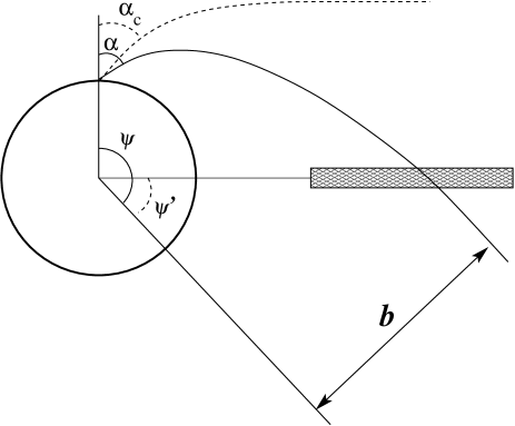
Figure 13: Trajectory of a photon in the gravitational field of a neutron star. Photons emitted at angle $\alpha>\alpha_{\rm c}$ relative to the stellar normal cross the disc plane.

We can estimate the inner disc radius independently from the observed amplitude of reflection. Let us assume that the emission originates from a small spot close to the rotational pole of the neutron star. (These assumptions give a lower limit on reflection amplitude.) Because of the light bending, a photon emitted at an angle $\alpha$ relative to the rotation axis, travels at the infinity along the trajectory which makes an angle $\psi$ with the axis (see Fig. 13). The relation between $\alpha$ and $\psi$ is given by an elliptical integral (Pechenick, Ftaclas & Cohen, 1983). At small $\alpha$, photons propagate in the upper hemisphere never crossing the disc plane. A photon emitted at a critical angle $\alpha_{\rm c}$ flies parallel to the disc surface. A simple estimate for this angle can be obtained using Beloborodov (2002, hereafter B02) approximation for light bending:

$$\cos\alpha=R_{\rm s}/R_{*}+(1-R_{\rm s}/R_{*})\cos\psi,$$ (2)

where $R_{*}$ is the stellar radius and $R_{\rm s}\equiv 2GM/c^{2}$ is the Schwarzschild radius for a star of mass $M$. Substituting $\psi=\pi/2$, we immediately get $\cos\alpha_{\rm c}=R_{\rm s}/R_{*}$. Photons, emitted at an angle $\alpha$ satisfying condition $0<\cos\alpha<R_{\rm s}/R_{*}$, will cross the disc plane at a radius given by an approximate expression for the photon trajectory (B02)

$$\frac{R_{\rm disc}(\alpha)}{R_{\rm s}}\approx\left[\frac{(1-\cos\psi^{\prime})^{2}}{4(1+\cos\psi^{\prime})^{2}}+\frac{b^{2}}{\sin^{2}\psi^{\prime}}\right]^{1/2}-\frac{1-\cos\psi^{\prime}}{2(1+\cos\psi^{\prime})},$$ (3)

where the impact parameter $b=R_{*}\ \sin\alpha/\sqrt{1-R_{\rm s}/R_{*}}$, $\psi^{\prime}=\psi-\pi/2$, and $\psi$ is related to $\alpha$ via equation (2). The smallest radius where photon trajectories can cross the disc is obtained by substituting $\alpha=\pi/2$, $\sin\psi^{\prime}=-1/(R_{*}/R_{\rm s}-1)$ and $b=R_{*}/\sqrt{1-R_{\rm s}/R_{*}}$ to equation (3).

We now can compute the reflection amplitude as a function of the inner disc radius. Let us assume for simplicity that radiation from the spot has a constant specific intensity $I(\alpha)=I_{0}=const$ (as for the black body emission). We can compute the luminosity (from the unit area) escaping to the infinity as

$$L_{\rm out}=2\pi\int_{0}^{\alpha_{\rm c}}I_{0}\cos\alpha\ \sin\alpha\ {\rm d}\alpha=\left[1-\left(\frac{R_{\rm s}}{R_{*}}\right)^{2}\right]\frac{I_{0}}{2}.$$ (4)

If the inner disc radius is larger than $R_{\rm disc}(\pi/2)$, we reverse relation (3) to find the emission angle $\alpha_{\rm in}$ at which a photon should be emitted to cross the disc at radius $R_{\rm in}$. The reflection luminosity is then

$$L_{\rm refl}=2\pi\int_{\alpha_{\rm c}}^{\alpha_{\rm in}}I_{0}\cos\alpha\ \sin\alpha\ {\rm d}\alpha=\left(\cos^{2}\alpha_{\rm c}-\cos^{2}\alpha_{\rm in}\right)\frac{I_{0}}{2}.$$ (5)

If $R_{\rm in}<R_{\rm disc}(\pi/2)$, the reflection luminosity is maximal $L_{\rm refl,max}=(R_{\rm s}/R_{*})^{2}I_{0}/2$.

In order to estimate the reflection amplitude, we need to specify the angular dependence of the observed escaping and reflected luminosities. The gravitational redshift affects both luminosities the same way and thus can be neglected. The escaping luminosity depends on the inclination angle as (see eq. [2]) $L_{\rm out}(i)\propto{R_{\rm s}/R_{*}+(1-R_{\rm s}/R_{*})\cos i}$, where normalization factor is found from the condition $L_{\rm out}=\int_{0}^{1}L_{\rm out}(i){\rm d}(\cos i)$. We can assume that the reflected luminosity is proportional to the disc area projected on the sky: $L_{\rm refl}(i)=L_{\rm refl}2\cos i$. Thus the reflection amplitude is:

$$\frac{\Omega}{2\pi}=\frac{L_{\rm refl}}{L_{\rm out}}\frac{(1+R_{\rm s}/R_{*})\cos i}{R_{\rm s}/R_{*}+(1-R_{\rm s}/R_{*})\cos i}\ .$$ (6)

It is plotted in Fig. 14 for different stellar compactnesses and inclination angles. Because the observed upper limit on the reflection amplitude is $\Omega/2\pi<0.07$ (see Section 4.2), the inner disc cannot be closer than about 90 km for inclination smaller than $60\degr$. At $i=80\degr$, constraints become much weaker and depend on stellar compactness. If stellar radius $R_{*}<2.5R_{\rm s}=10.5$ km (neutron star mass of $1.4{\rm M_{\odot}}$ was assumed), then $R_{\rm in}>40$ km, but if $R_{*}=3R_{\rm s}$ reflection is smaller (since bending is weaker) and any inner radius would satisfy these constraints.

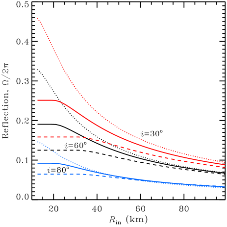
Figure 14: Reflection amplitude as a function of the inner disc radius. The source of photons is a small spot at the rotational pole of the neutron star. The intrinsic radiation pattern is assumed to be $I(\mu)=const$ (as for the black body emission). Dotted curves correspond to $R_{*}=2R_{\rm s}$, solid curves to $R_{*}=2.5R_{\rm s}$ and dashed curves to $R_{*}=3R_{\rm s}$. The upper curves are for the inclination $i=30\degr$, middle ones for $i=60\degr$, and the lower curves are for $i=80\degr$. Neutron star mass of 1.4 ${\rm M_{\odot}}$ is assumed.

Menna et al. (2003) estimated the magnetospheric radius for SAX J1808.4–3658 to be $\sim$17 km and argued that the accretion disc is disrupted at this radius. van Straaten, van der Klis & Wijnands (van Straaten et al.2004) analysed QPO frequency correlations in SAX J1808.4–3658 and found that the upper kilohertz QPO has a frequency by factor $\sim$1.5 lower when compared to other atoll sources, while low-frequency QPOs were comparable. They suggested that stronger magnetic field of SAX J1808.4–3658 moved the inner edge of the disc further away, and decreased the Keplerian frequency, responsible for the upper kHz QPO, while low-frequency QPOs were formed further out, and were not affected. There was no similar frequency shift in XTE J1751–305 (, van Straaten et al.2004), suggesting weaker magnetic field and smaller disruption radius than aforementioned 17 km.

Our results about the inner disc radius are not conclusive. The direct disc emission observed in the broad-band spectrum corresponded to the disc truncated close to the neutron star. This result depended on the assumed disc model and a radius of $\sim$ 40 km was possible for the disc without the torque-free inner boundary condition. Similar or larger radius was estimated from the rather small amount of Compton reflection from the disc. If the inner disc radius had been larger than the magnetospheric radius, it would have been truncated into an optically thin hot inner flow, similarly to the low/hard state of black holes (Shapiro et al., 1976; Esin et al., 1997). We would like to present an argument in favour of this scenario.

The low-frequency QPO and a break in the power spectrum are likely to be related to the truncation radius of the disc. The shape of the low-frequency power spectrum and frequency correlations are very similar in black holes and neutron stars (e.g. Wijnands & van der Klis, 1999), so their origin should be independent of the neutron star surface and magnetic field. The lack of correlation between the break/QPO frequency and the luminosity (see Figs. 1 and 12) supports this idea. If the disc were truncated at the magnetospheric radius indeed, we would expect its inner radius $R_{\rm in}=R_{\rm magn}\propto L^{-2/7}$, where $L$ is the luminosity (e.g. Hayakawa, 1985). Let us assume that the low-frequency QPO is connected to the precession time-scale of a vertical perturbation in the disc (Stella & Vietri, 1998; Psaltis & Norman, 2000). This yields $\nu_{\rm QPO}\propto R_{\rm in}^{-3/2}$, so we should expect $\nu_{\rm QPO}\propto L^{3/7}$. Any other link between the QPO frequency and the truncation radius would have resulted in the correlation between $\nu_{\rm QPO}$ and $L$. This has not been observed. Therefore the optically thick disc was probably truncated above the magnetospheric radius, by a mechanism independent of the magnetic field. This could be the same mechanism truncating the disc of the low/hard state in black hole binaries, e.g. evaporation (see Różańska & Czerny, 2000). The low-frequency part of the PDS is formed in this region. Below the truncation radius the disc is replaced by a hot, optically thin inner flow, which is eventually disrupted by the magnetic field at or near the magnetospheric radius.

8.3.2 Spot size

Let us estimate the physical size of the emission region using the model DBPF (hot shocked region surrounded by a cooler black body edges, see Fig. 2b) which seems physically more realistic. The inner spot area of $A\sim 20$ km² corresponds to the ‘observed’ at the infinity radius of $R_{\rm\infty}=2.5$ km. These estimations, however, do not take colour hardening and gravitational redshift and light bending into account.

The observed blackbody (i.e. colour) temperature is different from the effective temperature by a colour hardening factor, $f_{\rm col}\equiv T_{\rm col}/T_{\rm eff}$. For the hydrogen and helium atmospheres of weakly magnetized neutron stars, the exact value of the colour correction is not very well known, but it has been estimated to be $f_{\rm col}\sim$ 1.3 (Lewin, van Paradijs & Tamm, 1993; Zavlin, Pavlov & Shibanov, 1996; Madej, Joss & Różańska, 2004). This would result in a blueshift of the blackbody spectrum, and the effective radius of the blackbody would be $R_{\rm spot,eff}=f_{\rm col}^{2}R_{\rm\infty}$. Spectral hardening results from the fact that the absorption opacity rapidly decreases with increasing photon energy and one sees deeper and hotter layers at high energies. Situation in accreting pulsars can be quite opposite (see e.g. Deufel, Dullemond & Spruit, 2001): the hot layers are at the top and low-energy photons having larger absorption cross-section come from the hotter outer layers. It is possible that the resulting colour correction could be negligible, $f_{\rm col}\sim 1$.

Implementing gravitational corrections requires quite complicated numerical treatment. However, in the case when the (small) spot is always visible (which is the case for XTE J1751–305, because we observe almost sinusoidal oscillations) one can obtain a simple relation between the observed size at infinity and the physical size at the neutron star surface $R_{\rm spot}=R_{\rm\infty}Q^{-1/2}$ (B02; PG03), where $Q=R_{\rm s}/R_{*}+(1-R_{\rm s}/R_{*})\cos i\ \cos\theta$, and $\theta$ is the colatitude of the spot centre (magnetic inclination). The smallest possible radius is obtained for $i=\theta=0$, then $Q=1$ and $R_{\rm spot}=R_{\rm\infty}$. This corresponds to the minimum angular size of the spot of $\rho=12\degr$ ($14\degr$) for $R_{*}=3R_{\rm s}$ ($2.5R_{\rm s}$). A reasonable upper limit can be obtained taking $i=90\degr$ and $\theta=0$ (or $i=0$ and $\theta=90\degr$), now $Q=R_{\rm s}/R_{*}$ and $R_{\rm spot}=R_{\rm\infty}\sqrt{R_{*}/R_{\rm s}}$. (Note, that for the isotropically emitting star, the stellar radius is related to the observed radius as $R_{*}=R_{\rm\infty}\sqrt{1-R_{\rm s}/R_{*}}$, and is smaller than that.)

8.3.3 Constraints from the absence of the secondary maximum

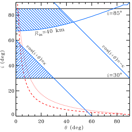
Figure 15: Constraints on the inclination and magnetic inclination of the system. The lines $i=30\degr$ and $i=85\degr$ are the lower and upper limits on the inclination of the system (M02). A small, $\rho=0$, antipodal spot is not visible in the region $\cos(i+\theta)>\kappa$ (below the corresponding line). A finite $\rho$ shifts this line further to the left by angle $\rho$. The primary spot is eclipsed sometimes when $\cos(i+\theta)<-\kappa$ (to the right from the corresponding line), and, therefore, is forbidden. Upper hatched area gives the allowed regions of parameters $i$ and $\theta$, where the antipodal spot is blocked by the disc of inner radius $R_{\rm in}=40$ km, and the primary spot is visible all the time. Contours of constant variability amplitude $A=0.045$ are shown for a black body spot (dashed curve, computed using Eq. 8) and for the spot radiation pattern corresponding to the 5th scattering order in a slab of Thomson optical depth $\tau_{\rm T}=1.5$ (dotted curve, numerical simulations for a pulsar of frequency 435 Hz). Neutron star of mass $M=1.4{\rm M_{\odot}}$ and radius $R_{*}=3R_{\rm s}$ is assumed.

The pulse profile of XTE J1751–305 is almost sinusoidal. This means that we see the emission from only one polar cap, as an antipodal spot would have created a secondary maximum (or a plateau) in the profile (e.g. B02, Viironen & Poutanen, 2004). At the same time, the primary spot should never be eclipsed by the star. The second shock can be obscured by the star or by the optically thick accretion disc. Let us consider first the possibility of obscuration by the star.

Obscuration by the star. The condition of obscuration of the secondary spot (class I in classification of B02) is $\cos\alpha_{\rm s}<0$. Using analytical formula for light bending (2) [$\psi=\psi_{\rm s}$ is now the angle between direction to the observer and normal to the secondary spot, $\cos\psi_{\rm s}=-(\cos i\ \cos\theta+\sin i\ \sin\theta\ \cos\phi$), and $\phi$ is the pulsar phase], we get $\cos(i+\theta)>\kappa$, where $\kappa\equiv R_{\rm s}/(R_{*}-R_{\rm s})$. For a more compact star, $R_{*}\lesssim 2R_{\rm s}$ (or about $1.8R_{\rm s}$ if exact bending formula is used), such a region does not exist at all.

In Fig. 15 we show an allowed region at the $i-\theta$ plane where obscuration is possible. We restrict the inclination of the system to lie in the interval $30\degr<i<85\degr$, as argued by M02. The hatched lower region corresponds to the allowed space of parameters $i-\theta$. One sees that the allowed region is rather small. It becomes even smaller, if we account for the finite spot size. The obscuration condition is then $\cos(i+\theta+\rho)>\kappa$, and the boundary of the region shifts further to the left by angle $\rho$ (i.e. by $\sim 15\degr$), further diminishing the allowed region. This region is smaller for more compact stars. Thus, we find that obscuration of the second spot by the star is highly improbable, unless the inclination is smaller than $30\degr$ and/or the stellar radius is larger than $3R_{\rm s}$. In that case, the inner disc radius has to be at least $\sim 200$ km, not to overproduce reflection.

The primary spot is eclipsed sometimes in the upper right corner of the diagram, $\cos(i+\theta)<-\kappa$ (i.e. $i+\theta>180\degr-\arccos\kappa$ – class III in B02 classification), and, therefore, is forbidden. Again for a spot of finite size, the limiting line shifts to the left by $\rho$.

Obscuration by the disc. Let us consider now obscuration of the secondary spot by the accretion disc. First, we need to compute radii $R_{\rm disc}$ at which photon orbits (reaching the observer) cross the disc plane. One can easily show that in flat space

$$R_{\rm disc}>R_{*}\sqrt{1+\cos^{2}\theta/\cos^{2}i}.$$ (7)

In Schwarzschild metrics, photon orbits cross the disc at somewhat larger radius due to the light bending. We computed numerically photon trajectories for every pulsar phase and found the minimum disc crossing radius. Now we can determine the region in the $i-\theta$ plane where this radius is larger than the disc inner radius which, as we argued above, is $R_{\rm in}\sim 40$ km (see Section 8.3.1). We show this region in Fig. 15 (upper hatched region, upper right boundary is determined by the condition of the visibility of the primary spot). We see that second spot is not visible only for inclinations above $\sim 67\degr$ (for $R_{*}=3R_{\rm s}$). Larger $R_{\rm in}$ will further reduce the allowed region.

If we account for the finite size of the spot, the allowed region shifts to the left by the angular size of the spot. However, the lower limit on the inclinations is not affected much, because now it is a rather flat function of $\theta$. We conclude that the second spot can be blocked by the accretion disc. We obtain constraints $i\gtrsim 67\degr$ ($i\gtrsim 70\degr$) and $\theta<30\degr$ ($\theta<35\degr$) for $R_{*}=3R_{\rm s}$ ($2.5R_{\rm s}$) for the spot size of $\rho\sim 15\degr$.

8.3.4 Constraints from the variability amplitude

Figure 16: Intensity (normalized to unity at $\mu=1$) of the radiation escaping from a slab of Thomson optical depth $\tau_{\rm T}=1.5$ for different scattering orders $n$ as a function of $\mu$ (here $\mu$ is the cosine of the zenith angle). The seed photons with intensity $I(\mu)=1$ are injected from the bottom of the slab. Calculation are done in Thomson scattering approximation (see Sunyaev & Titarchuk, 1985; Viironen & Poutanen, 2004).

Important constraints on the physical parameters of the system are given by the variability amplitude. The observed peak-to-peak amplitude $A\approx 0.045$ gives the minimum intrinsic variability. Let us first assume that all the emission comes the spot. For a slowly rotating star, the variability amplitude (for a black body spot) can be estimated from (B02; PG03):

$$A=U/Q,$$ (8)

where $U=(1-R_{\rm s}/R_{*})\sin i\ \sin\theta$. The dashed curve in Fig. 15 shows the relation between $i$ and $\theta$ satisfying the observed $A$.

In reality, the star rotates rapidly and the radiation pattern from of the Comptonized emission is far from the black body. Rapid rotation causes a slight shift of the maximum emission from the phase where projected area has the maximum towards the phase where Doppler factor has a maximum (i.e. quarter of the period earlier, see PG03). Additionally, light travel time delays skew the profile.

Change in the emission pattern causes even larger changes to the oscillation profile. The angular dependence of the radiation escaping from a slab of Thomson optical depth $\tau_{\rm T}=1.5$ (as suggested by spectral fitting, see Section 4.3 and Table 4) is shown in Fig. 16 (see also Viironen & Poutanen, 2004). It depends on the scattering order $n$ which is in turn related to the photon energy as $E/3kT_{\rm seed}\approx(1+4kT_{\rm e}/m_{\rm e}c^{2})^{n}$. Thus we expect 3–7 scatterings to contribute most of the flux in the PCA range. As an example we compute the light curves expected for $n=5$ using fully relativistic method described in PG03 and Viironen & Poutanen (2004). Contour plots at the $i-\theta$ plane for $A=0.045$ are shown in Fig. 15 by dotted curves. We see that the Comptonized emission produces smaller variability compared to the black body, and for the same $i$, larger $\theta$ is needed to get the same amplitude.

If we take the upper hatched region as the allowed region of parameters, we immediately get that the magnetic pole is misaligned from the rotational pole by a very small angle, $\theta=3-4\degr$. This angle becomes larger if it is only a fraction of the emission that comes from the spot.

8.4 Distance

We used the distance of 8.5 kpc throughout this paper, assuming that the source is close to the Galactic centre. M02 placed XTE J1751–305 at a distance of at least 7 kpc, using indirect arguments. There are, however, clues that this distance might be actually much smaller.

Firstly, the source is very bright, $L_{\rm peak}=0.13L_{\rm Edd}$, when placed at 8.5 kpc. It is about an order of magnitude brighter than SAX J1808.4–3658, while all other properties are very similar. At higher accretion rates, typically more that a few per cent of the Eddington limit, atoll sources switch to a soft (banana) spectral state (e.g. Hasinger & van der Klis, 1989). This is not the case here. But the transition luminosity can be quite high, in particular during the onset of the outburst, where hysteresis effect has been observed and the source can remain in the hard state despite high accretion rate (Maccarone & Coppi, 2003). For example, Aql X-1 and 4U 1705–44 have been observed in the hard island state at luminosities $\sim$ 20 per cent of $L_{\rm Edd}$ (Barret & Olive, 2002; Done & Gierliński, 2003). Therefore, having XTE J1751–305 in the hard state at 13 per cent of the Eddington luminosity cannot be ruled out.

Cumming, Zweibel & Bildsten (2001) argued that the crucial difference between the millisecond pulsars and non-pulsating atolls was in the average accretion rate (related to the size of the disc, which is smaller in the millisecond pulsars). In atolls, the accretion rate is high enough to bury the magnetic field under the surface. The diffusion time-scale of rebuilding the field is $\sim$1000 years, much larger than a typical period between the outbursts. In millisecond pulsars the accretion rate, $\dot{m}$, is never high enough to bury the field. Cumming et al. (2001) estimated that magnetic screening is ineffective for $\dot{m}<0.02\dot{m}_{\rm Edd}$. Then, 0.13 $L_{\rm Edd}$ would have been too much for the magnetic field to survive in XTE J1751–305 during the outburst. It would need $D\la 3$ kpc for $\dot{m}$ to be low enough for the field not to be buried. This issue would require further study to resolve.

If XTE J1751–305 were located at $D$ = 3 kpc indeed, it would decrease the blackbody apparent areas quoted in Table 4 by factor $(8.5/3)^{2}\approx 8$ and disc inner radius by factor $8.5/3\approx 3$. The model DBPS (and DBTH), where the seed photons were from the blackbody component, would give the blackbody area of $\sim$100 km, and could not be rejected on the spot size basis. The inner spot area in DBPF model would be $\sim$3 km² and its linear size derived in Section 8.3.2 would be less by factor $\sim$3.

9 Summary

We have analysed the 2002 outburst of the second accretion-powered millisecond pulsar XTE J1751–305. The broad-band 0.7–200 keV spectrum of XTE J1751–305 obtained by XMM-Newton and RXTE is complex. The best-fitting models consist of two soft components and thermal Comptonization. Most likely the cooler soft component comes from the accretion disc, the hotter one from the surface of the neutron star, while Comptonization takes place in a shocked region in the accretion column. We estimate the electron temperature of the plasma 30–40 keV and Thomson optical depth $\tau\sim 1.5$ (for a slab geometry). In our best spectral models, the temperature of the seed soft photons for Comptonization is higher than the temperature of the visible soft blackbody component which is consistent with a picture where photons from a heated spot under the shock are scattered away by the shocked plasma. In this model, the ‘observed’ (at the infinity) area of the blackbody emission is about 100 km² corresponding to a spot of radius $\sim$ 5–6 km. The area corresponding to a shock was estimated to be 20 km², which translates to a radius of 2.5-4.5 km depending on the assumed compactness of the neutron star and the viewing angle.

The analysis of the RXTE spectra obtained during the outburst shows that temperature of the soft blackbody photons as well as the temperature of the seed photons decreased monotonically. The spectral slope of the hard Comptonized component did not vary much. We argued that this favours a constant geometry (e.g. slab) emission region and two-phase models, where energy is dissipated in the hot phase and the seed photons for Comptonization are the result of reprocessing of the hard X-rays.

The pulse profile cannot be fitted by a simple sinusoid, a second harmonic is required. The mean peak-to-peak amplitude of the first and second harmonic is about 4.5 and 0.15 per cent, respectively. There is a clear energy dependence of the profile, the amplitude gradually decreases and the peak at higher energies appears at earlier phases (soft lags). The time lags reach $\sim 100$ $\mu{\rm s}$ and seem to saturate at about 10 keV. This behaviour is almost identical to SAX J1808.4–3658 where lags are factor of two larger. The observed energy dependence of the pulse profiles can be explained by a model where blackbody and Comptonization components vary sinusoidally with a small phase shift. Such a behaviour can result from the Doppler boosting and different angular distribution of the emission from these components (PG03).

The non-detection of the reflected component in the time-averaged spectra and the absence of the emission from the second antipodal spot (we see almost sinusoidal variations) put constraints on the geometry of the system. We argued that the inner radius of the optically thick accreting disc is about 40 km. In that case, the secondary can be blocked by the accretion disc if the inclination of the system is larger than $\sim 70\degr$. Blockage of the secondary by the star itself is highly unlikely for the neutron star radii $R_{*}<3R_{\rm s}$. The observed variability amplitude constrain the magnetic pole to lie within 3–4$\degr$ of the rotational pole, if most of the observed X-ray emission comes from a hotspot and a shock.

References

- Agol & Krolik (2000) Agol E., Krolik J. H., 2000, ApJ, 528, 161
- Aly & Kuijpers (1990) Aly J. J., Kuijpers J., 1990, A&A, 227, 473
- Arnaud (1996) Arnaud K. A., 1996, in Jacoby G. H., Barnes J., eds, Astronomical Data Analysis Software and Systems V. ASP Conf. Series Vol. 101, San Francisco, p. 17
- Barret (2001) Barret D., 2001, Adv. Space Res., 28, 307
- Barret & Olive (2002) Barret D., Olive J.-F., 2002, ApJ, 576, 391
- Barret & Vedrenne (1994) Barret D., Vedrenne G., 1994, ApJS, 92, 505
- Basko & Sunyaev (1976) Basko M. M., Sunyaev R. A., 1976, MNRAS, 175, 395
- Beloborodov (2002) Beloborodov A. M., 2002, ApJ, 566, L85 (B02)
- Bhattacharya (1995) Bhattacharya D., 1995, in Lewin W. H. G., van Paradijs J., van den Heuvel E. P. J., eds, X-ray Binaries, Cambridge University Press, Cambridge, p. 233
- Cui et al. (1998) Cui W., Morgan E. H., Titarchuk L. G., 1998, ApJ, 504, L27
- Cumming et al. (2001) Cumming A., Zweibel E., Bildsten L., 2001, ApJ, 557, 958
- Cunningham (1975) Cunningham C. T., 1975, ApJ, 202, 788
- Davis et al. (2004) Davis S. W., Blaes O. M., Hubeny I., Turner N. J., 2004, ApJ, submitted (astro-ph/0408590)
- Deufel et al. (2001) Deufel B., Dullemond C. P., Spruit H. C., 2001, A&A, 377, 955
- Done & Gierliński (2003) Done C., Gierliński M., 2003, MNRAS, 342, 1041
- Eckert et al. (2004) Eckert D., Walter R., Kretschmar P., Mas-Hesse M., Palumbo G.G.C., Roques J.-P., Ubertini P., Winkler C., 2004, ATel 352
- Esin et al. (1997) Esin A. A., McClintock J. E., Narayan R., 1997, ApJ, 489, 865
- Galeev et al. (1979) Galeev A. A., Rosner R., Vaiana G. S., 1979, ApJ, 229, 318
- Galloway et al. (2002) Galloway D. K., Chakrabarty D., Morgan E. H., Remillard R. A., 2002, ApJ, 576, L137
- Galloway et al. (2005) Galloway D. K., Markwardt C. B., Morgan E. H., Chakrabarty D., Strohmayer T. E., 2005, astro-ph/0501064
- Gierliński & Done (2002) Gierliński M., Done C., 2002, MNRAS, 337, 1373
- Gierliński & Done (2004) Gierliński M., Done C., 2004, MNRAS, 347, 885
- Gierliński et al. (1999) Gierliński M., Zdziarski A. A., Poutanen J., Coppi P. S., Ebisawa K., Johnson W. N., 1999, MNRAS, 309, 496
- Gierliński et al. (2002) Gierliński M., Done C., Barret D., 2002, MNRAS, 331, 141 (GDB02)
- Gilfanov et al. (1998) Gilfanov M., Revnivtsev M., Sunyaev R., Churazov E., 1998, A&A, 338, L83
- Haardt & Maraschi (1993) Haardt F., Maraschi L., 1993, ApJ, 413, 507
- Hasinger & van der Klis (1989) Hasinger G., van der Klis M., 1989, A&A, 225, 79
- Hayakawa (1985) Hayakawa S., 1985, Phys. Rep., 121, 317
- Kompaneets (1956) Kompaneets A. S., 1956, Soviet Phys., JETP, 31, 876
- Lewin et al. (1993) Lewin W. H. G., van Paradijs J., Taam R., 1993, Sp. Sci. Rev., 62, 223
- Lyubarskii & Sunyaev (1982) Lyubarskii Yu. E., Sunyaev R. A., 1982, SvA Lett., 8, 330
- Maccarone & Coppi (2003) Maccarone T., Coppi P. S., 2003, MNRAS, 338, 189
- Madej et al. (2004) Madej J., Joss P. C., Różańska A., 2004, ApJ, 602, 904
- Malzac et al. (2001) Malzac J., Beloborodov A. M., Poutanen J., 2001, MNRAS, 326, 417
- Markwardt & Swank (2003) Markwardt C. B., Swank J. H., 2003, IAUC, 8144, 1
- Markwardt et al. (2003) Markwardt C. B., Smith E., Swank J. H., 2003, IAUC, 8080, 2
- Markwardt et al. (2002) Markwardt C. B., Swank J. H., Strohmayer T. E., in ’t Zand J. J. M., Marshall F. E., 2002, ApJ, 575, L21 (M02)
- Markwardt et al. (2004) Markwardt C. B., Swank J. H., Strohmayer T. E., 2004, ATel 353
- Menna et al. (2003) Menna M. T., Burderi L., Stella L., Robba N., van der Klis M., 2003, ApJ, 589, 503
- Miller et al. (2003) Miller J. M. et al., 2003, ApJ, 583, L99
- Mitsuda et al. (1984) Mitsuda K., Inoue H., Koyama K. et al., 1984, PASJ, 36, 741
- Nowak (2000) Nowak M. A., 2000, MNRAS, 318, 361
- Pechenick et al. (1983) Pechenick K. R., Ftaclas C., Cohen J. M., 1983, ApJ, 274, 846
- Poutanen (2004) Poutanen J., 2004, in Kaaret P., Lamb F. K., Swank J. H., eds, X-ray Timing 2003: Rossi and Beyond, AIP, Melville, NY, p. 228
- Poutanen & Gierliński (2003) Poutanen J., Gierliński M., 2003, MNRAS, 343, 1301 (PG03)
- Poutanen & Svensson (1996) Poutanen J., Svensson R., 1996, ApJ, 470, 249
- Psaltis & Norman (2000) Psaltis D., Norman C., 2000, astro-ph/0001391
- Romanova et al. (2004) Romanova M. M., Ustyugova G. V., Koldoba A. V., Lovelace R. V. E., 2004, ApJ, 610, 920
- Różańska & Czerny (2000) Różańska A., Czerny B., 2000, A&A, 360, 1170
- Shahbaz et al. (1998) Shahbaz T., Charles P. A., King A. R., 1998, MNRAS, 301, 382
- Shapiro et al. (1976) Shapiro S. L., Lightman A. P., Eardley D. M., 1976, ApJ, 204, 187
- Shimura & Takahara (1995) Shimura T., Takahara F., 1995, ApJ, 445, 780
- Stella & Vietri (1998) Stella L., Vietri M., 1998, ApJ, 492, L59
- Stern et al. (1995) Stern B. E., Poutanen J., Svensson R., Sikora M., Begelman M. C., 1995, ApJ, 449, L13
- Sunyaev & Titarchuk (1985) Sunyaev R. A., Titarchuk L. G., 1985, A&A, 143, 374
- van Straaten et al. (2002) van Straaten S., van der Klis M., di Salvo T., Belloni T., 2002, ApJ, 568, 912
- (57) van Straaten S., van der Klis M., Wijnands R., 2004, Nucl. Phys. B. (Proc. Suppl.), 132, 664
- Viironen & Poutanen (2004) Viironen K., Poutanen J., 2004, A&A, 426, 985
- Wijnands & van der Klis (1998a) Wijnands R., van der Klis M., 1998a, Nat, 394, 344
- Wijnands & van der Klis (1998b) Wijnands R., van der Klis M., 1998b, ApJ, 507, L63
- Wijnands & van der Klis (1999) Wijnands R., van der Klis M., 1999, ApJ, 514, 939
- Zavlin et al. (1996) Zavlin V. E., Pavlov G. G., Shibanov Yu. A., 1996, A&A, 315, 141
- Zdziarski, Johnson & Magdziarz (1996) Zdziarski A. A., Johnson W. N., Magdziarz P., 1996, MNRAS, 283, 193
- Zhang, Cui & Cheng (1997) Zhang S. N., Cui W., Chen W., 1997, ApJ, 482, L155
- Życki et al. (1998) Życki P., Done C., Smith D. A., 1998, ApJ, 496, L25