Cosmic microwave background constraints on dark energy dynamics: analysis beyond the power spectrum

Abstract

We consider the distribution of the non-Gaussian signal induced by weak lensing on the primary total intensity cosmic microwave background (CMB) anisotropies. Our study focuses on the three point statistics exploiting an harmonic analysis based on the CMB bispectrum. By considering the three multipoles as independent variables, we reveal a complex structure of peaks and valleys determined by the re-projection of the primordial acoustic oscillations through the lensing mechanism. We study the dependence of this system on the expansion rate at the epoch in which the weak lensing power injection is relevant, probing the dark energy equation of state at redshift corresponding to the equivalence with matter or higher ($w_{\infty}$). The variation of the latter quantity induces a geometrical feature affecting distances and growth rate of linear perturbations, acting coherently on the whole set of bispectrum coefficients, regardless of the configuration of the three multipoles. We evaluate the impact of the bispectrum observable on the CMB capability of constraining the dark energy dynamics. We perform a maximum likelihood analysis by varying the dark energy abundance, the present equation of state $w_{0}$ and $w_{\infty}$. We show that the projection degeneracy affecting a pure power spectrum analysis in total intensity is broken if the bispectrum is taken into account. For a Planck-like experiment, assuming nominal performance, no foregrounds or systematics, and fixing all the parameters except $w_{0}$, $w_{\infty}$ and the dark energy abundance, a percent and ten percent precision measure of $w_{0}$ and $w_{\infty}$ is achievable from CMB data only. The reason is the enhanced sensitivity of the weak lensing signal to the behavior of the dark energy at high redshifts, which compensates the reduced signal to noise ratio with respect to the primary anisotropies. These results indicate that the detection of the weak lensing signal by the forthcoming CMB probes may be relevant to gain insight into the dark energy dynamics at the onset of cosmic acceleration.

I INTRODUCTION

Explaining the cosmic acceleration represents one of the greatest challenges of modern cosmology. A reliable candidate for the dark energy, a vacuum energy density similar to the Cosmological Constant and responsible for the acceleration, should provide an answer to the fine-tuning and the coincidence problem. The fine-tuning is required to adjust the vacuum energy to the observed level, about 123 orders of magnitude lower than the Planck energy scale. The coincidence question is simply why the observed vacuum energy is comparable to the critical energy density today (see lambda_review and references therein).

A class of models proposed to explain the cosmic acceleration invoques a scalar field playing the role of the dark energy, minimally or non-minimally coupled to dark matter or gravity (see e.g. de_models and references therein). Despite of the variety of the theoretical frameworks, all these models predict a time-varying equation of state for the dark energy, usually represented through its value at a given time, plus the first derivative in redshift or cosmological scale factor linder ; polarski .

The dark energy equation of state is being constrained by a number of experiments, such as Type Ia supernovae (SNIa) which have been the first evidence for cosmic acceleration sn1a , as well as Cosmic Microwave Background (CMB) wmap and Large Scale Structure (LSS) tegmark . The CMB total intensity power spectrum in particular is sensitive to the dark energy equation of state mainly through a projection effect induced by the variation of the distance to the last scattering surface bacci ; since the latter is a redshift integral between the present and last scattering, it washes out any sensitivity to the time dependence of the dark energy equation of state, probing just its redshift average.

A crucial benchmark in the era of precision cosmology is the measure of the redshift behavior of the dark energy equation of state, fixing the cosmological observables which are able to probe it at the epoch of equivalence with matter or earlier, where most models predict significant differences. A number of future probes aim at this goal, including the Planck satellite (http://www.rssd.esa.int/PLANCK), the planned CMB polarization mission, as well as observation of SNIa from space perlsnap jointly with weak lensing surveys (see e.g. refregier04 and references therein). The latter effect in particular, i.e. the weak lensing induced on the background light by forming structures is one of the most promising probes to investigate the whole dark cosmological component, matter and energy, and is gathering an increasing theoretical and observational interest (see e.g. wl_review ); in particular, the weak lensing is potentially relevant to investigate the high redshift behavior of the dark energy, since the onset of cosmic acceleration overlaps in time with structure formation.

In this work we consider the effect of the weak lensing on CMB anisotropies. The theory of this process has been casted in the context of the linear cosmological perturbation theory hu , and recently extended to cosmologies involving a scalar field dark energy component with generalized kinetic energy and coupling to the Ricci scalar acquaviva . In particular, we concentrate on the non-Gaussian distortion induced through the lensing effect on the CMB total intensity anisotropies. An attempt to detect this signal relating the data from the Wilkinson Microwave Anisotropy Probe (WMAP) and the galaxy distribution in the Sloan Digital Sky Survey (SDSS) has been done recently without success hirata . This effect is usually described in terms of the power injection in the CMB third order statistics, represented in the harmonic domain by the CMB bispectrum (see spergel_goldberg ; komatsu and references therein); its relevance in constraining the redshift average of the dark energy equation of state has been studied in detail verde . In our previous work giovi we pointed out that the bispectrum weak lensing signal is a promising probe of the high redshift behavior of the dark energy, independently on the present regime of acceleration. We studied the redshift distribution of the weak lensing power injection in the CMB bispectrum in equilateral configuration, demonstrating that it is vanishing at zero and infinity, being relevant at intermediate redshift only, when cosmic acceleration takes place. In this work we study the structure of the whole bispectrum power from weak lensing, and set up a maximum likelihood analysis fixing all cosmological parameters except those related to the dark energy, to show how the bispectrum enhanced sensitivity to the high redshift behavior of the expansion rate can be used to break the projection degeneracy affecting the CMB power spectrum.

The paper is structured as follows: in Sec. II we set our framework by defining the dark energy parameterization and recalling the basic aspects of the calculation of the CMB bispectrum signal from weak lensing; in Sec. III we analyze the tri-dimensional multipole distribution of the bispectrum signal; in Sec. IV we perform a likelihood analysis on simulated power spectrum and bispectrum CMB data; in Sec. V we make our concluding remarks.

II DARK ENERGY, WEAK LENSING AND CMB BISPECTRUM

It is now well understood that a dark energy component would mainly affect the total intensity power spectrum of the CMB anisotropies through a projection effect on the acoustic peaks bacci . Indeed, the dark energy dynamics may potentially alter the distance to the last scattering surface, which provides a way to estimate the dark energy content and its equation of state from CMB measurements if a suitable dark energy model is given. In a different approach, one could instead use CMB observations as a tool to infer the underlying dark energy properties, without assuming its dynamics following the prediction of a specific model. In this case linder ; polarski , it is convenient to parameterize the evolution of the dark energy equation of state as

$$w(z)=w_{0}+(w_{\infty}-w_{0})\frac{z}{1+z}\ ,$$ (1)

where $w_{0}$ and $w_{\infty}$ are, respectively, the present and the asymptotic ($z\rightarrow\infty$) values of the dark energy equation of state. This is not the only parameterization, see for instance corasaniti03 , but it is enough for our purposes here. Note that the difference $(w_{\infty}-w_{0})$ corresponds to the parameter $w_{a}$ in the original notation linder . For reference, in giovi , we analyzed two scalar field dark energy models which, at the level of background evolution, are very well reproduced by appropriate choices of $w_{0}$ and $w_{\infty}$. The parameterization (1) misses the fluctuations in the dark energy scalar field, although that is not necessary here as we address the dependence of the CMB three point statistics on the background expansion rate. The comoving distance to the last scattering surface can be written as

$$r(z_{lss})=\frac{c}{H_{0}}\int_{0}^{z_{lss}}\frac{dz}{\sqrt{\Omega_{m}(1+z)^{3}+\Omega_{V}e^{f(z)}}}\ ,$$ (2)

where

$$f(z)=3\int_{0}^{z}dz^{\prime}\frac{1+w(z^{\prime})}{1+z^{\prime}}\ .$$ (3)

In Eq. (2) we have restricted our analysis to a flat universe and neglected radiation; $c$ is the speed of light, $H_{0}$ denotes the Hubble constant, $z_{lss}$ is the redshift of last scattering surface and $\Omega_{m}=\Omega_{b}+\Omega_{cdm}$ is the matter density today ($\Omega_{b}$ and $\Omega_{cdm}$ are respectively the baryon energy density and the cold dark matter energy density). The dark energy density is simply $\Omega_{V}=1-\Omega_{m}$.

However, reconstructing the behavior of $w(z)$ through the shift induced on the CMB acoustic peaks turns out to be a complicate task: as pointed out in verde , the analysis of the power spectrum alone is affected by a degeneracy between the dark energy equation of state and $\Omega_{V}$. Such degeneracy becomes worse when the dark energy dynamics is taken into account; typically, in the latter case at least another parameter is introduced, as in Eq. (1): even assuming $\Omega_{V}$ perfectly known, the two redshift integrals prevent from measuring $w_{0}$ and $w_{\infty}$ separately from the CMB power spectrum only. The use of higher order statistics giovi or a cross correlation between several observables (see e.g. corasaniti04 ) is needed to break this degeneracy.

Under the assumption of initial Gaussian conditions, the CMB non-Gaussian diffuse signal is mainly generated by the cross-correlation between the gravitational lensing and the Integrated Sachs-Wolfe (ISW) effect. Such correlation causes a non-vanishing power in the three point statistics, which may be described in terms of the CMB bispectrum.

The three product of the harmonic expansion coefficients of the CMB anisotropies in total intensity may be ensemble averaged to get the bispectrum power on the angular scales specified by a triplet of multipoles; the projected lensing potential allows to write down the bispectrum dependence on the power spectrum of scalar perturbations (see e.g. verde ); the result is

$$B_{l_{1}l_{2}l_{3}}=\sqrt{\frac{\left(2l_{1}+1\right)\left(2l_{2}+1\right)\left(2l_{3}+1\right)}{4\pi}}\left(\begin{array}[]{ccc}l_{1}&l_{2}&l_{3}\\ 0&0&0\end{array}\right)\cdot$$ (6)

$$\cdot\frac{l_{1}\left(l_{1}+1\right)-l_{2}\left(l_{2}+1\right)+l_{3}\left(l_{3}+1\right)}{2}C_{l_{1}}^{lss}Q\left(l_{3}\right)+5P\ ,$$ (7)

where the parenthesis denote Wigner 3J symbols, $C_{l_{1}}^{lss}$ is the primordial power spectrum of total intensity anisotropies, and $5P$ indicates five permutation over the three multipoles. $Q(l)$ is produced by the cross correlation between the gravitational lensing and the ISW signal, expanded in spherical harmonics spergel_goldberg ; verde :

$$Q(l)\simeq 2\int_{0}^{z_{lss}}dz\frac{r\left(z_{lss}\right)-r(z)}{r\left(z_{lss}\right)r^{3}(z)}\left[\frac{\partial P_{\Psi}(k,z)}{\partial z}\right]_{k=\frac{l+1/2}{r(z)}}\ .$$ (8)

Above the gravitational potential power spectrum is given by $P_{\Psi}(k,z)=\left(\frac{3}{2}\Omega_{m}\right)^{2}(H_{0}/ck)^{4}P(k,z)(1+z)^{2}$ where $P(k,z)$ is the density power spectrum. We evaluate the contribution of non-linearity to the matter power spectrum using the semi-analytical approach of ma ; for a complete derivation of Eq. (6) and Eq. (8) see giovi ; verde and references therein.

In writing Eq. (8), we used the Limber approximation; that is widely used in the literature (see afs and references therein) and we perform here a numerical check of its validity. In the calculations leading to (6), one faces the product of spherical Bessel functions. Those are suitably replaced by the relation

$$j_{l}(x)=\sqrt{\frac{\pi}{2l+1}}\left[\delta\left(l+\frac{1}{2}-x\right)+\Delta_{l}(x)\right]\ ,$$ (9)

where $\delta$ is the Dirac’s delta and the function $\Delta_{l}(x)$, represents the difference between the Bessel function and the Dirac delta itself; when integrating (9) with regular functions, one finds that the contribution from $\Delta_{l}$ vanishes at high $l$s as $l^{-2}$. The Limber approximation consists in neglecting the contributions of the $\Delta_{l}$ terms, which allows to get to (8). More precisely, by substituting (9) into the expression of the lensing-ISW correlation, one gets

$$Q_{true}(l) = Q(l)+(2l+1)\left\{\int\frac{dr}{r^{3}}\frac{r_{lss}-r}{r_{lss}r}\int dr_{1}\Delta_{l}(x)|_{x=(l+\frac{1}{2})\frac{r_{1}}{r}}\left[\Psi(k,r)\frac{\partial\Psi(k,r_{1})}{\partial r_{1}}\right]_{k=\frac{l+1/2}{r}}+\right.$$ (10)

$$+ \left.\int dr\frac{r_{lss}-r}{r_{lss}r}\int\frac{dr_{1}}{r_{1}^{3}}\Delta_{l}(x)|_{x=(l+\frac{1}{2})\frac{r}{r_{1}}}\left[\Psi(k,r)\frac{\partial\Psi(k,r_{1})}{\partial r_{1}}\right]_{k=\frac{l+1/2}{r_{1}}}\right\}+\mathcal{O}(l^{-3})\ ,$$

where $\Psi(k,r)$ is the cosmological gravitational potential, defined as the metric fluctuations in absence of anisotropic stress; the underlying assumption of Gaussian distribution of cosmological perturbations eliminates one of the two integrals in the Fourier wavenumbers. The last term, representing the error on $Q(l)$, presents an overall behavior as $l^{-1}$, coming from the combination of $\Delta_{l}$ and the $2l+1$ term in front of the integral. We quantified the error induced by the Limber approximation by computing $Q(l)$ with and without that, considering a $\Lambda$CDM cosmological model consistent with the WMAP first year data wmap . We find an error which is about $1\%$ at $l=10$, falling down approximately as $1/l$ afterwards as predicted by our expectation (10); we stress that $l=10$ is the lowest multipole considered in our analysis, as it was done before (see verde ) in order not to approach too low multipoles where the Limber approximation may not be satisfactory. Our results are also consistent with afs , quoting a $2-3\%$ error at $l=3$, corresponding to about $1\%$ at $l=10$ with an $1/l$ scaling, as we find. In conclusion, we verify that the Limber approximation holds at percent or better in our analysis, and we exploit that in the rest of the work.

III THE STRUCTURE OF THE TRI-DIMENSIONAL BISPECTRUM

In this Section, we investigate the physical properties and phenomenology of the weak lensing bispectrum signal in its most general configuration.

In giovi , only “equilateral” geometries were considered (i.e., $l_{1}=l_{2}=l_{3}$ in Eq. (6)): however, as we discuss in the following, it is greatly restrictive to consider that configuration only, expecially from the point of view of the signal to noise ratio. As discussed in detail in hu , the cosmic variance and instrumental noise act on the $B_{l_{1}l_{2}l_{3}}$ elements essentially as a three product of the sum $C_{l}^{lss}+C_{l}^{noise}$, where the last term represents the instrumental noise contribution. Therefore, the bispectrum signal to noise ratio is defined as

$$\left(\frac{S}{N}\right)^{2}=\sum_{l_{1},l_{2},l_{3}}\frac{B_{l_{1}l_{2}l_{3}}^{2}}{n_{l_{1}l_{2}l_{3}}C_{l_{1}}C_{l_{2}}C_{l_{3}}}\ ,$$ (11)

where the constant $n_{l_{1}l_{2}l_{3}}$ is $6$ for equilateral configurations, $2$ if two multipoles are equal (isosceles triangles) and $1$ if all multipoles are different (scalene triangles). Note that, in order to make use of the small angle approximation verde , we have to adopt a lower limit on $l$, indicated as $l_{min}$; as in giovi we fix $l_{min}=10$ in the following. The results do not depend at all on this choice. From Eq. (11) we see that in the equilateral configuration we are summing $l_{max}$ terms, while in the most general case the signal to noise ratio receives contributions from about $l_{max}^{3}$ terms: for this reason, it is clear that the “scalene” configuration contains much more information, just because the sum (11) is dominated by those coefficients.

As it is evident in equation (6), the weak lensing relates the primordial signal $C_{l}^{lss}$ and the lensing kernel given in (8) on different scales. The first exhibits an oscillatory, decaying behavior around $l^{-2}$, at least for $l\lesssim 1000$ i.e. before the damping tail; the second is a straight power law decaying faster, followed by a change of sign and a shallower decay occurring on the scale of a few hundreds in $l$ as a result of the domination of the non-linear tail in the density power spectrum giovi . The combination of the two behaviors, as a general function of the three multipoles, distributes the oscillatory power of $C_{l}^{lss}$ on scales different from the ones of the primordial acoustic oscillations, creating a complex pattern of peaks and valleys which is the recurring feature of the weak lensing bispectrum signal. Such structure is not distributed over the whole $(l_{1},l_{2},l_{3})$ space, since geometrical constraints greatly reduce the avaliable domain. A physical constraint making the signal vanishing is represented by the transition from linear to non-linear power domination in (8).

It is convenient to give an illustration of that phenomenology providing an example of tri-dimensional view of the bispectrum signal; in Fig. 1 we plot the absolute value of the bispectrum coefficients for a cosmological model with $\Omega_{V}=0.73$, $w_{0}=-1$ and $w_{\infty}=-0.8$; the remaining cosmological parameters are set accordingly to the cosmic concordance model, $H_{0}=72$ km/s/Mpc, $\Omega_{b}=0.046$, $\Omega_{cdm}=1-\Omega_{V}-\Omega_{b}$, reionization optical depth $\tau=0.11$, scalar perturbations only with spectral index $n_{s}=0.96$. The signal is dimensionless ($Q(l)$ is a number and $C_{l}^{lss}\propto(\delta T/T)^{2}$) and valid for a cosmology with $\Omega_{V}=0.73$, $w_{0}=-1$ and $w_{\infty}=-0.8$, corresponding to our fiducial model as we explain later. The first thing to note is that the bispectrum is vanishing for multipoles triplets which do not satisfy the triangular relation (Wigner 3J symbols are zero) as well as for configurations where the sum of multipoles is odd. In the case shown, $Q\left(l_{3}\right)=0$; a variation of $l_{3}$ changes the regions where the triangularity relation is not verified: if $l_{3}$ is increased, the bispectrum domain is squeezed along the direction $l_{1}=l_{2}$ and is stretched in the orthogonal direction; if $l_{3}$ is decreased, we obtain the opposite behavior.

The two main features discussed above are well evident. First, the sort of “canyon” representing the fingerprint of the transition between the linear and non-linear regime in the power spectrum derivative in (8), yielding a change of sign appearing “cuspidal” in module; a “valley” appears close and aligned with the left border of the bispectrum domain, this time determined entirely by the behavior of the signal which is rising at the lowest multipoles giovi . Second, the re-projection of the acoustic oscillations due to the mixing (6): the whole power in the central region of the figure, roughly between the valley and the canyon, comes mainly from the first acoustic oscillation in the power spectrum, which gets projected on a large domain of multipole triplets, i.e. angular scales. The phenomenology is therefore markedly richer with respect to the case of the ordinary power spectrum. On the other hand, the weak lensing signal is a second order effect in terms of cosmological perturbations, and the cosmic variance alone does not allow the detection of the single bispectrum coefficient. Nevertheless, a satisfactory signal to noise ratio is achieved by summing over all the different configurations.

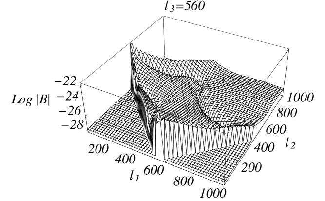
Figure 1: Example of distribution of tri-dimensional bispectrum coefficients. The domain is determined by geometrical constraints in the Wigner symbols, while the “canyon” is due to the transition between linear and non-linear power in the density power spectrum. The primordial acoustic oscillations are projected on multiple angular scales by the weak lensing effect.

The tri-dimensional information may be compressed in several ways; a uni-dimensional quantity which contains the contributions from all the possible configurations is

$$B_{l_{1}}=\sum_{l_{2},l_{3}=l_{min}}^{l_{max}}B_{l_{1}l_{2}l_{3}}\ ,$$ (12)

where we take $l_{min}=10$ and $l_{max}=1000$. In Fig. 2 we plot $B_{l_{1}}$. The figure is representative of the angular scales from which the signal takes most of the contribution, which are close to the maximum primordial power in the first acoustic peak. This is consistent with previous analysis spergel_goldberg . The remaining part of the signal is made of a relevant part at low multipoles, probably due to the rise of the overall bispectrum power (see Fig. 1), plus a series of oscillations with varying amplitudes. The latter seem still related to the series of peaks in the primordial power. Finally, the positive and negative high frequency oscillations are entirely due to the behavior of the 3J Wigner symbols.

Figure 2: Bispectrum in units of $10^{-20}$ as function of the multipole $l_{1}$ only, obtained by marginalization over $l_{2}$ and $l_{3}$. The small scale, negative and positive oscillations are due to the Wigner 3J symbols. The large scale modulation is instead a physical feature related to the primordial acoustic peaks.

The information described in Fig. 1 and 2 is totally compressed when the signal to noise ratio, defined in (11), is computed. It is shown in Fig. 3 for three cases: two years WMAP nominal noise, two years Planck nominal noise (as in Table 1 in balbi ) and cosmic variance only; all the cases considered do not take into account systematics and foregrounds, and an all sky coverage is assumed. The plateau means that no extra information is added extending the sum (11) at very high $l$s, where the signal vanishes below cosmic variance and noise. WMAP is cosmic variance limited up to $l\simeq 300$, while Planck up to $l\simeq 1000$. Of course this discussion does not take into account foreground or systematics contamination, which in practice may represent major obstacles against the actual detection. In the following, we consider only the effect of cosmic variance, and probe the bispectrum up to $l_{max}\simeq 1000$; the results are therefore representative of an experiment with the nominal performance of Planck.

Figure 3: Bispectrum signal to noise ratio as function of $l_{max}$ for a cosmic variance limited experiment (solid line), Planck two years nominal noise (short dashed line) and WMAP two years nominal noise (long dashed line). The cosmology corresponds to our fiducial model with $\Omega_{V}=0.73$, $w_{0}=-1$ and $w_{\infty}=-0.8$; the other parameters are fixed accordingly to the cosmic concordance model.

IV COMBINING POWER SPECTRUM AND BISPECTRUM: LIKELIHOOD ANALYSIS AND RESULTS

In this Section, we discuss how the bispectrum data improve the CMB sensitivity to the high redshift behavior of the dark energy.

As already mentioned, the power spectrum suffers the degeneracy of the comoving distance to last scattering surface relatively to different values of the dark energy parameters. One of the most important aspects of the CMB bispectrum from weak lensing is the fact that it correlates the primordial temperature anisotropies with later physical processes, i.e. the formation of structures), probing the dark energy behavior at that epoch giovi .

Let us describe here our likelihood analysis. Most of the cosmological parameters are fixed according to the cosmological concordance model; we shall perform only a variation of the dark energy parameters $\Omega_{V}$, $w_{0}$ and $w_{\infty}$, which allows us to build a grid of $C_{l}$ and $Q(l)$ values. Then, spanning over our parameter space, we calculate the bispectrum by mean of the relation (6). Once we have that as a function of $\Omega_{V},w_{0}$ and $w_{\infty}$, we compute a three parameters likelihood both for the power spectrum and for the bispectrum; the combined analysis is simply obtained by multiplying the two of them.

The other cosmological parameters are set to their values for our fiducial model, described earlier. We evaluate the likelihood as usual as

$$\mathcal{L}_{s,b}=A_{s,b}\exp\left(-\frac{\chi_{s,b}^{2}}{2}\right)\ ,$$ (13)

where the subscripts refer, respectively, to the power spectrum $(s)$ and to the bispectrum $(b)$, $A_{s,b}$ is a normalization factor and $\chi_{s,b}^{2}$ are functions of the dark energy parameters defined as

$$\chi_{s}^{2} = \sum_{l=2}^{1000}\left[\frac{C_{l}^{t}-C_{l}^{f}}{\sigma_{l}^{s}}\right]^{2}\ ,$$ (14)

$$\chi_{b}^{2} = \sum_{l_{1},l_{2},l_{3}=10}^{1000}\left[\frac{B_{l_{1}l_{2}l_{3}}^{t}-B_{l_{1}l_{2}l_{3}}^{f}}{\sigma_{l_{1}l_{2}l_{3}}^{b}}\right]^{2}\ .$$ (15)

In the expression above, we describe spectrum and bispectrum as Gaussian variables gangui ; takada : that corresponds to ignore the possible non-Gaussianity arising in the early universe, as well as to assume a Gaussian distribution for the bispectrum coefficients, exploiting the argument which states that in the case of weak lensing the signal is caused by many independent events. The superscript $t$ refers to the theoretical model, while $f$ refers to our fiducial model. As we already mentioned, we limit our analysis to multipoles smaller than 1000, being consistent with a Planck-like experiment with nominal performance (see Fig. 3). For the power spectrum, the well known expression of the cosmic variance is $\left(\sigma_{l}^{s}\right)^{2}=2/(2l+1)C_{l}^{2}$; for the bispectrum, $\left(\sigma_{l_{1}l_{2}l_{3}}^{b}\right)^{2}=n_{l_{1}l_{2}l_{3}}C_{l_{1}}C_{l_{2}}C_{l_{3}}$. We also neglect the correlation between the two observables as it is induced by higher order statistics takada , which allows us to write down the combined likelihood as

$$\mathcal{L}_{c}=\mathcal{L}_{s}\mathcal{L}_{b}=A_{c}\exp\left(-\frac{\chi_{s}^{2}+\chi_{b}^{2}}{2}\right)\ ,$$ (16)

where $A_{c}$ normalizes the combined likelihood.

We report the results of our likelihood analysis in three main cases, with one, two and three free parameters. As we show later this approach is necessary to understand how different the basins of degeneracy of spectrum and bispectrum are, and how their combination actually break the projection degeneracy affecting the power spectrum. We use the following priors: $0\leq\Omega_{V}\leq 1$, $-1\leq w_{0}\leq-0.6$, $-1\leq w_{\infty}\leq-0.6$. When $\Omega_{V}$ varies, the matter abundance is changed to keep flatness and leaving $\Omega_{b}$ unchanged.

IV.1 One parameter likelihood

This is the simpler case, where two of the three dark energy parameters are fixed to their fiducial values, while the third one is allowed to vary. In that case, regardless of which parameter varies, the bispectrum doesn’t improve the likelihood analysis of the power spectrum alone. The reason is simply the reduced signal to noise ratio of the bispectrum. When just one parameter vary, even $w_{\infty}$, the tiny changes in the power spectrum signal dominate the exponential in the combined likelihood; note that when $w_{\infty}$ varies, the relative changes in the bispectrum are stronger than in the power spectrum case giovi . However, when the noise is taken into account, such advantage is canceled and the joint likelihood is almost identical to $\mathcal{L}_{s}$. As we shall see in the next sub-section, the results change greatly when a multi-dimensional analysis is performed. The reason is that the basins of degeneracy of spectrum and bispectrum open in markedly different ways, making their combination advantageous.

IV.2 Two parameters likelihood

Here we analyze the likelihood behavior with respect to the variation of two dark energy parameters.

Let’s begin by fixing $\Omega_{V}=0.73$; though the power spectrum likelihood is very narrow (see Fig. 4 left panel), it is degenerate along a specific direction, where different values of $w_{0}$ and $w_{\infty}$ produce similar values of the function $e^{f(z)}$ in Eq. (2) at the epoch of the structure formation. For this reason, the power spectrum is able to exclude a wide region of the parameter space, but it is unable to constrain $w_{0}$ and $w_{\infty}$ separately. The bispectrum likelihood is non-zero over a wider region of the parameter space, but vanishes on the region where the power spectrum is degenerate (Fig. 4 center panel); while the projection degeneracy affecting the power spectrum is well understood, it is more difficult to track the dark energy variables in the bispectrum calculation, as they enter in several aspects, i.e. distances and perturbation growth. The only clear feature is the vanishing of the lensing power at present and infinity giovi , making the bispectrum sensitive to $w_{\infty}$ more than to $w_{0}$, as in Fig. 4; the likelihood shape, rather elongated on the $w_{0}$ direction, and sharper on the $w_{\infty}$ one, is clearly consistent with our expectation. As a result, the degeneracy basins of spectrum and bispectrum are misaligned, allowing the separate measure of $w_{0}$ and $w_{\infty}$ from their combination (Fig. 4, right panel). In the left panel of Fig. 5 we show the contour plot of the power spectrum and bispectrum likelihoods; as we can see, the gain is evident.

In the center panel and in the right one of Fig. 5 we show the contour levels of the other two likelihood analysis, fixing $w_{0}$ and $w_{\infty}$ respectively. In those cases, getting the bispectrum into the analysis does not improve substantially the constraints. The reason is that fixing one parameter in the exponential $e^{f(z)}$ in Eq. (2) virtually break the power spectrum projection degeneracy: more specifically, separate changes in $w_{0}$ or $w_{\infty}$ cannot be compensated by changes in $\Omega_{V}$, since the latter changes the matter abundance, inducing changes in the power spectrum shape which again dominate the exponential in the joint likelihood. As we shall see now, the latter reasoning does not apply when all the three parameters vary, causing a relevant gain for all of them in the combined analysis.

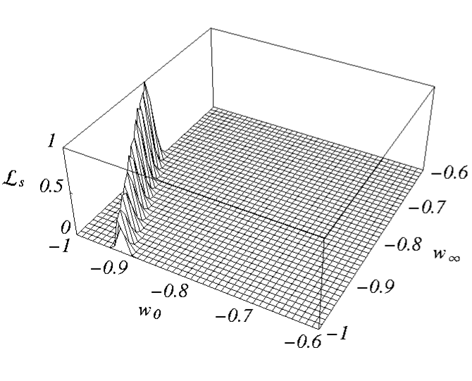
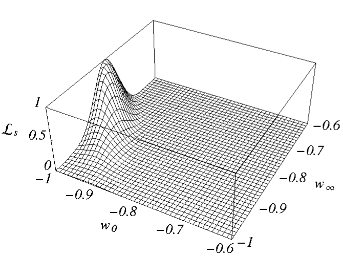
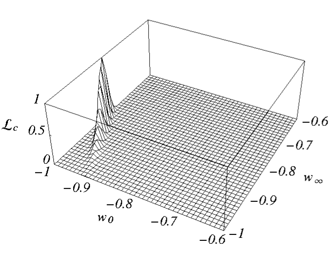
Figure 4: Likelihoods as function of $w_{0}$ and $w_{\infty}$ with $\Omega_{V}=0.73$; from left to right: power spectrum only, bispectrum only and their combination.

Figure 5: Likelihood confidence levels at $1\sigma$ (innermost contours) and $2\sigma$ (outermost contours) for power spectrum only (solid line) and for power spectrum and bispectrum (dashed line). From left to right: marginalization over $\Omega_{V}$, marginalization over $w_{0}$, marginalization over $w_{\infty}$. The dot is the fiducial model and it is located at $(\Omega_{V}=0.73,w_{0}=-1,w_{\infty}=-0.8)$.

IV.3 Three parameters likelihood

In Fig. 6, 7 and 8 we plot the three parameters likelihoods marginalized respectively over $\Omega_{V}$, $w_{0}$ and $w_{\infty}$; in each figure, the top-left panel is the power spectrum likelihood, the top-right panel is the bispectrum likelihood, the bottom-left panel is the combined likelihood and in the bottom-right panel we put the contour plots at $2\sigma$ and $1\sigma$ confidence levels for the power spectrum likelihood and the combined one.

As expected, when marginalizing over $\Omega_{V}$, the likelihood analysis gives almost the same result as when $\Omega_{V}$ is fixed (see Sec. IV.2). Indeed, the leading feature is the projection degeneracy in the CMB power spectrum with respect to combined variation of $w_{0}$ and $w_{\infty}$; the latter gets worse when also $\Omega_{V}$ varies, although the latter variation affects also the matter abundance inducing relevant changes in the power spectrum; the resulting picture is therefore almost equivalent to the case when $\Omega_{V}$ is fixed.

However, the three parameters case is different with respect to the previous one when the marginalization is performed over $w_{0}$ or $w_{\infty}$. In the previous sub-section we saw that when $w_{0}$ or $w_{\infty}$ is fixed, the power spectrum constraints dominate the joint likelihood. As we discussed above, having one of the two dark energy equation of state parameters fixed means breaking the projection degeneracy for the power spectrum, when also $\Omega_{V}$ varies. In the present case the latter argument disappears, and the power spectrum constraints are still fully affected by that degeneracy, causing the visible gain from having the bispectrum into the analysis.

The top panels of Fig. 7, obtained marginalizing over $w_{0}$, reveal two different weaknesses of spectrum and bispectrum, which make their combination fruitful. First, the weak sensitivity of the power spectrum to $w_{\infty}$: the likelihood is almost flat for a long line in the $w_{\infty}$ direction, until the latter parameter induces a change strong enough to let the likelihood vanishing. On the other hand, the sensitivity to $\Omega_{V}$ is strong as its variation affects the matter abundance, inducing important changes in the power spectrum shape. The opposite happens for the bispectrum. Now the preferred parameter is $w_{\infty}$, as it determines the dark energy behavior at the time when the lensing power is injected. This orthogonality in the degeneracy direction of spectrum and bispectrum determines the great advantage of their combination, clearly visible in the bottom panels of Fig. 7.

The minimum gain is got in the case of Fig. 8, where the marginalization is made on $w_{\infty}$. Indeed, the latter operation washes out the parameter of greatest importance for the bispectrum; in the top-right panel, the bispectrum degeneracy direction roughly corresponds to the constancy of the dark energy abundance at the time in which the lensing injects its power. On the other hand, as we stressed above the gain is still relevant and visible in the bottom panels of Fig. 8, as the three parameters analysis makes the power spectrum projection degeneracy fully effective.

In Fig. 9 we give a qualitative picture of the different likelihood shapes for spectrum and bispectrum, in the three parameters analysis, where one has been marginalized; the solid and dashed lines represent the power spectrum and bispectrum likelihoods, respectively; they are normalized to their maximum values and the five contours for each observable are equally spaced between 0 and 1 to highlight their shape.

Finally, to quantify how the bispectrum analysis improves the estimation of the dark energy parameters, we report in Tab. I the constraints (both at $1\sigma$ and $2\sigma$) on our parameters, obtained when the power spectrum, bispectrum and the combined analysis are applied to our fiducial model. We stress that the other cosmological parameters are kept fixed. This table refers to the three parameter likelihoods, marginalized over the remaining two of them. As discussed, the confidence levels are always narrower when the bispectrum analysis is added to the power spectrum one. Roughly, the precision on the measures of $w_{0}$ and $w_{\infty}$ is percent and ten percent, respectively.

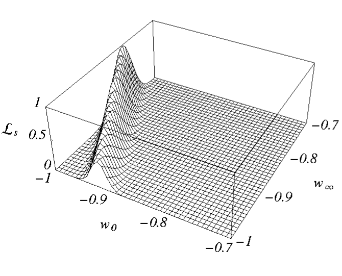
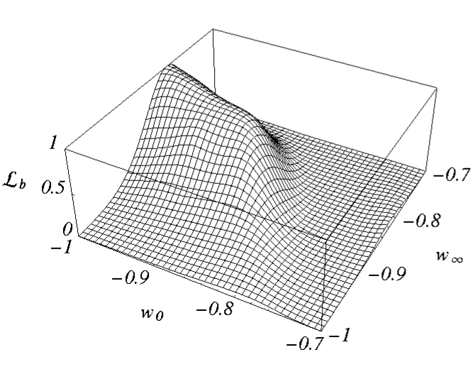
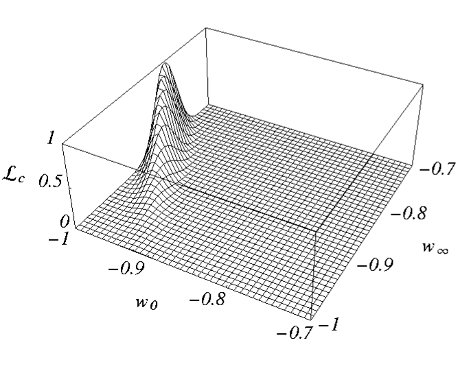
Figure 6: Likelihood marginalized over $\Omega_{V}$ for the power spectrum only (top-left), bispectrum only (top-right) and both (bottom-left). In the bottom-right panel we plot the contour levels at $1\sigma$ (innermost contours) and $2\sigma$ (outermost contours) for the power spectrum by itself (solid line) and combined with the bispectrum (dashed line), the dot is our fiducial model.

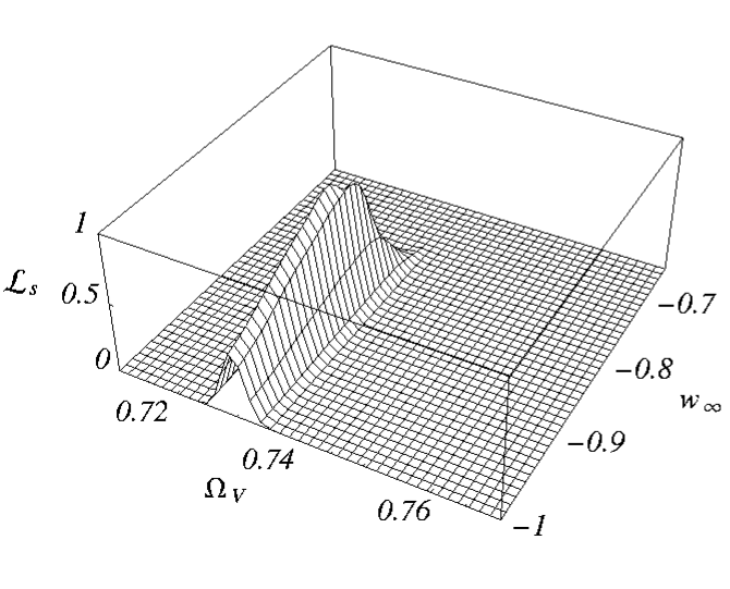
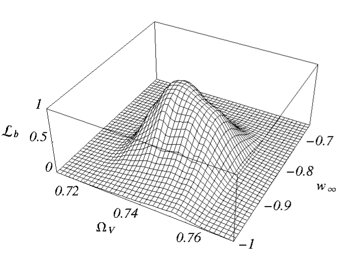
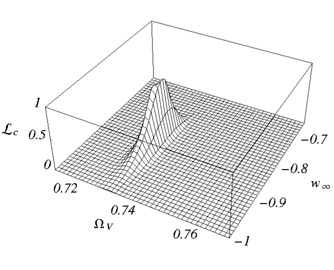
Figure 7: As in Fig. 6 but with marginalization over $w_{0}$.

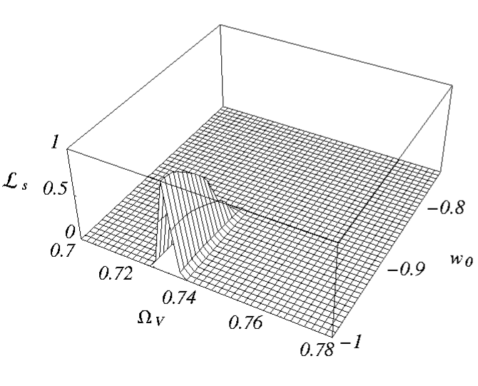
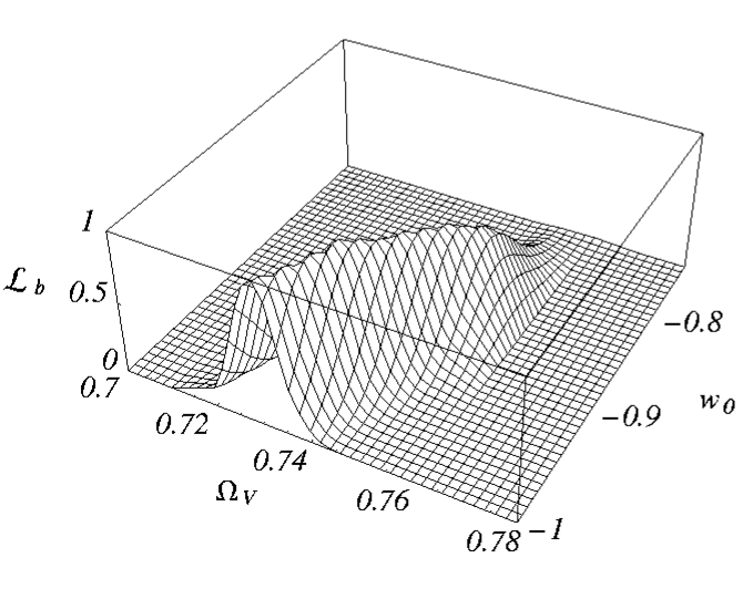
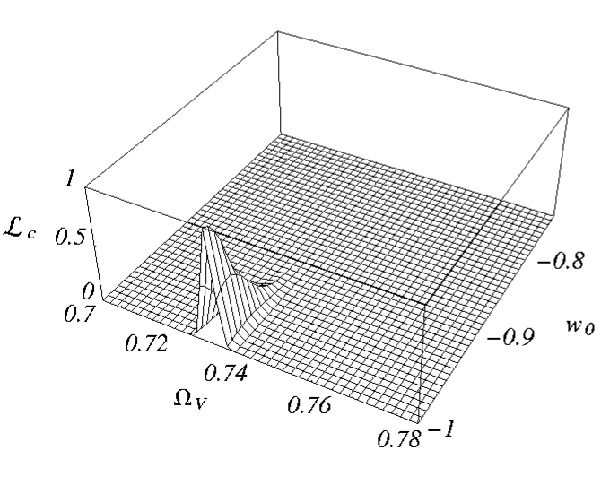
Figure 8: As in Fig. 6 but with marginalization over $w_{\infty}$.

Figure 9: Contour levels for the three parameters analysis, where one has been marginalized; the solid and dashed lines represent the power spectrum and bispectrum likelihoods, respectively; they are normalized to their maximum values and the five contours for each observable are equally spaced between 0 and 1 showing qualitatively the different basins of degeneracy. From left to right: marginalization over $\Omega_{V}$, marginalization over $w_{\infty}$, marginalization over $w_{0}$.

Table 1: Confidence level at $1\sigma$ and $2\sigma$ of marginalized three parameters likelihood.

$1\sigma$ c.l.	$\Omega_{V}$	$w_{0}$	$w_{\infty}$
Power spectrum	$0.728\leq\Omega_{V}\leq 0.732$	$w_{0}\leq-0.95$	$-0.94\leq w_{\infty}\leq-0.81$
Bispectrum	$0.731\leq\Omega_{V}\leq 0.750$	$w_{0}\leq-0.89$	$-0.89\leq w_{\infty}\leq-0.78$
Combined	$0.729\leq\Omega_{V}\leq 0.732$	$w_{0}\leq-0.97$	$-0.87\leq w_{\infty}\leq-0.80$
$2\sigma$ c.l.	$\Omega_{V}$	$w_{0}$	$w_{\infty}$
Power spectrum	$0.727\leq\Omega_{V}\leq 0.734$	$w_{0}\leq-0.92$	$w_{\infty}\leq-0.79$
Bispectrum	$0.724\leq\Omega_{V}\leq 0.759$	$w_{0}\leq-0.79$	$-0.96\leq w_{\infty}\leq-0.74$
Combined	$0.727\leq\Omega_{V}\leq 0.734$	$w_{0}\leq-0.94$	$-0.93\leq w_{\infty}\leq-0.77$

V CONCLUSIONS

We studied the non-Gaussian signal induced on the Cosmic Microwave Background (CMB) total intensity anisotropies by weak gravitational lensing, and its dependence on the redshift behavior of the cosmological expansion rate. Our approach is based on the harmonic expression of the three point CMB anisotropy statistics, which is conveniently described in terms of the CMB bispectrum.

The lensing bispectrum signal depends on a triplet of angular multipoles, connecting the primordial signal with the lensing kernel; the latter is expressed through a redshift integral probing the redshift derivative of the primordial power spectrum of density perturbations on different scales projecting the same angle along the line of sight. Such connection, appearing as a product of the primordial signal and the lensing kernel on different multipoles, determines a re-projection of the acoustic peaks on scales markedly different from their well known location in the CMB power spectrum. The bispectrum coefficients, seen as a function of the three multipoles in arbitrary configuration, depict a complex structure of peaks and valleys in a tri-dimensional space, bounded by geometrical constraints encoded in the Wigner 3J symbols. A recurring feature is the presence of a sign inversion in the bispectrum coefficients, on angular scales of a few hundreds, cutting almost in the middle the whole signal distribution; the latter feature represent the transition between linear and non-linear power domination in the lensing kernel, and appears visually as a “canyon” in the distribution of the absolute value of the bispectrum coefficients verde ; giovi .

Although rich, this phenomenology is unfortunately not observable in detail, as the effect represents a second order cosmological perturbation, and the single coefficient is largely dominated by cosmic variance. The only way to exploit practically the bispectrum coefficients is to compress the information by summing over the different multipole triplets. By doing that, we verified that most of the signal is contained in the triplets with different values of the multipoles (“scalene” configurations), merely because they represent the large majority of the whole number of coefficients. We evaluated the signal to noise ratio by summing over all the triplets as a function of the maximum multipole in the sum. In agreement with previous analyses hu , we show how a cosmic variance limited experiment should be able to detect the bispectrum signal by summing at least up to a maximum multipole of a few hundreds.

As it is known from previous works, the lensing signal is injected at redshift higher than the present, and is therefore promising as a probe of the expansion rate at that epoch. We parameterized the redshift behavior of the expansion rate by means of the dark energy abundance relative to the critical cosmological density today, $\Omega_{V}$, its present and high redshift equation of state, $w_{0}$ and $w_{\infty}$, respectively linder . For CMB studies, the expectation giovi is that the bispectrum data may increase the overall sensitivity of the CMB on the dark energy high redshift dynamics, represented by $w_{\infty}$, in comparison with the usual analysis made on the basis of the CMB total intensity power spectrum only; the latter is sensitive to the redshift average of the dark energy equation of state, through a projection effect: different combinations of $w_{0}$ and $w_{\infty}$ leading to the same redshift average cannot be distinguished.

To assess to what level such degeneracy is broken by taking into account the CMB bispectrum, we set up a maximum likelihood analysis simulating a Planck-like experiment, varying $\Omega_{V}$, $w_{0}$ and $w_{\infty}$ and keeping all the other cosmological parameters fixed to our fiducial model. Despite of the lower signal to noise ratio, the bispectrum likelihood contours present a substantial misalignment with respect to those of the power spectrum, being more sensitive to changes in $w_{\infty}$; this is consistent with the expectation quoted above, i.e. that the lensing should probe directly the expansion rate at the epoch when the process is effective, independently on the present. The bispectrum actually breaks the degeneracy of the CMB on the redshift behavior of the dark energy, allowing a detection of both $w_{0}$ and $w_{\infty}$, at least in our three parameters likelihood analysis, where those and the dark energy abundance are the only varying parameters; the level of accuracy is at percent and ten percent, respectively. These results may increase the interest and efforts toward the detection of the weak lensing signal by the forthcoming CMB probes, as that may be relevant to gain insight into the dark energy dynamics at the onset of cosmic acceleration, when most models similar to a Cosmological Constant at present predict very different behaviors.

A number of caveats or potential obstacles should be pointed out here against this expectation.

Our analysis is based on a few parameters only, directly related to the dark energy. Of course a multi-parameter study would possibly reveal dangerous degeneracies in the bispectrum dependence on the underlying cosmology. On the other hand, the CMB spectrum by itself, as well as the wealth of independent cosmological observations are fixing with high accuracy the main cosmological parameters. Such accuracy will even increase with the observations by the forthcoming probes. In this framework, it is reasonable to conceive focused analyses based on specialized observables to probe critical aspects of the whole cosmological picture. A study of this kind focused on the dark energy dynamics would fit in this category: that would involve the non-Gaussian CMB signal injected by the weak lensing and its relation with the redshift behavior of the cosmological expansion rate, but would take place within the confidence region allowed to the the remaining cosmological parameters by the collection of cosmological observations.

Another important aspect concerns directly the lensing kernel. As we stressed above, a relevant part of the bispectrum signal comes from the non-linear tail in the cosmological perturbation power spectrum. The reliability of any constraint coming from this observable depend crucially on the correct modeling of that part of the spectrum. Although several recipes have been proposed and currently used in many applications, this issue would deserve a particular attention as a crucial piece of the constraining power of the non-Gaussian CMB signal from lensing.

Also, the early universe itself may be a source of non-Gaussianity in the primary CMB signal, and the weak lensing distortion should be compared with the corresponding one from non-Gaussian models of primordial perturbations.

Moreover, even if the cosmological uncertainties mentioned above are under control, the foreground astrophysical signals may affect the final result and need to be controlled. Due to the weakness of the signal, both diffuse Galactic foregrounds and extra-Galactic point sources or Sunyaev-Zel’Dovich (SZ) effects might be dangerous. A study of the foreground non-Gaussian signal in comparison to the CMB one from weak lensing will be certainly possible as the CMB observations are providing an excellent improvement on our knowledge of the foreground emission. Some very preliminary considerations may be attempted concerning the first evidence of non-zero bispectrum signal from radio sources wmap_ps , as well as the predicted SZ signal and the possible contribution from the early universe, which have been reviewed recently bartolo . Specifically, we evaluated the amplitude of the lensing signal with respect to those in figure 14 in the latter work; this indicates that it dominates over the radio sources and SZ contributions, which are significant at high angular scales, where we do not add more information by adding terms in the sum in Eq. (6). On the other hand, the signal seems comparable with the level of non-Gaussianity allowed by the present experiments in the early universe wmap_ps . This is a very naive indications that the extra-Galactic foregrounds may not be dramatic as a contaminant of the lensing signal; the same indications, extended to all foregrounds, has been reported independently hirata ; that is supported by the fact that some control of foregrounds may be achieved exploiting their different scaling in frequency with respect to the CMB in multi-band observations wmap_ps . On the other hand, a major contaminant, if present, may be represented by the primordial non-Gaussianity, and one should exploit its different shape with respect to the lensing signal in order to detect both independently.

Finally, almost all the known instrumental systematics, including sky cut, are a source on non-Gaussianity in the observed CMB pattern. Although the future probes promise an excellent control of systematics, the instrumental performance should be checked against the cosmological signal also for what concerns higher order statistics in the CMB pattern.

Despite of all these issues, and in the light of the results presented above, it is certainly worth to address these caveats to assess their relevance for CMB bispectrum measurements. Indeed, cosmic acceleration constitutes a pillar of the whole cosmological picture, although not understood. Any observable probing the transition to acceleration may be crucial to spread light on it in the forthcoming years.

References

- (1) P.J.E. Peebles and B. Ratra, Rev. Mod. Phys. 75, 599 (2003); T. Padmanabhan, Phys. Rep. 380, 235 (2003).
- (2) L. Amendola, Phys. Rev. D69, 103524 (2004); S. Matarrese, C. Baccigalupi and F. Perrotta, Phys. Rev. D 70, 061301(R), (2004).
- (3) E.V. Linder, Phys. Rev. Lett., 90, 091301 (2003).
- (4) M. Chevallier and D. Polarski, Int. J. Mod. Phys. D 10, 213 (2001).
- (5) A.G. Riess et al., Astrophys. J. 116, 1009 (1998); S. Perlmutter et al., Astrophys. J. 517, 565 (1999).
- (6) D.N. Spergel et al., Astrophys. J. Suppl. Series 148, 175 (2003).
- (7) M. Tegmark et al., Phys. Rev. D69, 103501 (2004).
- (8) C. Baccigalupi, A. Balbi, S. Matarrese, F. Perrotta and N. Vittorio, Phys. Rev. D65, 063520 (2002).
- (9) S. Perlmutter, Nucl. Phys. B Proc. Suppl., 124, 13 (2003)
- (10) A. Refregier et al., Astron.J. 127, 3102 (2004).
- (11) M. Bartelmann and P. Schneider, Phys. Rep. 340, 291 (2001); A. Refregier, Ann. Rev. Astron. Astrophys. 41, 645 (2003).
- (12) W. Hu, Phys. Rev. D 62, 043007 (2000).
- (13) V. Acquaviva, C. Baccigalupi and F. Perrotta, Phys. Rev. D 70, 023515 (2004).
- (14) C.M. Hirata, N. Padmanabhan, U. Seljak, D. Schlegel and J. Brinkmann, Phys. Rev. D70, 103501 (2004).
- (15) D.N. Spergel and D.M. Goldberg, Phys. Rev. D 59, 103001 (1999); D.M. Goldberg and D.N. Spergel, Phys. Rev. D 59, 103002 (1999).
- (16) E. Komatsu and D. N. Spergel, Phys. Rev. D63, 063002 (2001).
- (17) L. Verde and D.N. Spergel, Phys. Rev. D 65, 043007 (2002).
- (18) F. Giovi, C. Baccigalupi and F. Perrotta, Phys. Rev. D 68, 123002 (2003).
- (19) P.S. Corasaniti and E.J. Copeland, Phys. Rev. D67, 063521, (2003).
- (20) P.S. Corasaniti, M. Kunz, D. Parkinson, E.J. Copeland and B.A. Bassett, Phys. Rev. D70, 083006 (2004); H.K. Jassal, J.S. Bagla and T. Padmanabhan, preprint astro-ph/0404378, to appear in Mon. Not. R. Astron. Soc. Lett., (2004); B. Gold, preprint astro-ph/0411376, submitted to Phys. Rev. D (2004).
- (21) C.P. Ma, Astrophys. J. Lett. 508, L5, (1998); C.P. Ma, R.R. Caldwell, P. Bode and L. Wang, Astrophys. J. Lett 521, L1 (1999).
- (22) N. Afshordi, Y.S. Loh and M.A. Strauss, Phys. Rev. D69, 083524 (2004).
- (23) A. Balbi, C. Baccigalupi, F. Perrotta, S. Matarrese and N. Vittorio, Astrophys. J. Lett. 588, L5 (2003).
- (24) Gangui A. and Martin J., Mon. Not. R. Astron. Soc. 313, 323 (2000).
- (25) M. Takada and B. Jain, Mon. Not. R. Astron. Soc. 348, 897 (2004).
- (26) Komatsu et al., Astrophys. J. Supp. Series, 148, 119, (2003).
- (27) Bartolo N., Komatsu E., Matarrese S., Riotto A., Phys. Rep. 402, 103 (2004).