The age of the Galactic thin disk from Th/Eu nucleocosmochronology

The purpose of this work is to resume investigation of Galactic thin disk dating using nucleocosmochronology with Th/Eu stellar abundance ratios, a theme absent from the literature since 1990. [Th/Eu] abundance ratios for a sample of 20 disk dwarfs/subgiants of F5 to G8 spectral type with $-0.8\leq\mathrm{[Fe/H]}\leq+0.3$, determined in the first paper of this series, were adopted for this analysis. We developed a Galactic chemical evolution model that includes the effect of refuse, which are composed of stellar remnants (white dwarfs, neutron stars and black holes) and low-mass stellar formation residues (terrestrial planets, comets, etc.), contributing to a better fit to observational constraints. Two Galactic disk ages were estimated, by comparing literature data on Th/Eu production and solar abundance ratios to the model ($8.7^{+5.8}_{-4.1}\leavevmode\nobreak\ \mbox{Gyr}$), and by comparing [Th/Eu] vs. [Fe/H] curves from the model to our stellar abundance ratio data (($8.2\pm 1.9)\leavevmode\nobreak\ \mbox{Gyr}$), yielding the final, average value $(8.3\pm 1.8)\leavevmode\nobreak\ \mbox{Gyr}$. This is the first Galactic disk age determined via Th/Eu nucleocosmochronology, and corroborates the most recent white dwarf ages determined via cooling sequence calculations, which indicate a low age ($\lesssim 10\mbox{ Gyr}$) for the disk.

1 Introduction

Current estimates of the age of the Galactic thin disk are obtained by dating the oldest open clusters or white dwarfs. Ages of open clusters are determined by fitting isochrones, and ages of white dwarfs are determined using cooling sequences. Isochrone and cooling sequence calculations require deep knowledge of stellar evolution, are very complex, and depend on a large number of physical parameters known at different levels of uncertainty. Many important aspects of stellar evolution, like the influence of rotation, are not well known, and may have a strong influence on the outcome of isochrone calculations. Furthermore, white dwarf cooling sequences also depend on calculations of degenerate-matter physics. Nucleocosmochronology is a dating method that makes use of only a few results of main sequence stellar evolution models, therefore allowing a quasi-independent verification of the afore mentioned techniques.

Nucleocosmochronology estimates timescales for astrophysical objects and events by using abundances of radioactive nuclides. These are compared with the abundances of their daughter nuclides, or of other nuclides that are created by the same or a similar nucleosynthetic process. Depending on the half-life of the chosen nuclide, different timescales can be probed. The Th/Eu chronometer, first proposed by Pagel (1989), is adequate to assess the age of the Galactic disk, since $\@element[232]{\mathrm{T}}$h is a radioactive nuclide with a 14.05 Gyr half-life (i.e., of the order of magnitude of the age being assessed). Eu is a satisfactory element for comparison, because it is produced almost exclusively (97%, according to Burris et al. 2000) by the same nucleosynthetic process that produces all Th, the rapid neutron-capture process (r-process).

Since Sneden et al. (1996) carried out the first Th/Eu nucleocosmochronological dating of an ultra-metal-poor (UMP) star, the literature has been virtually dominated by these objects (Truran et al. 2002, and references therein). The reason for such interest lies in the strong simplifications that can be applied to the dating of UMP stars, which does not require the use of Galactic chemical evolution (GCE) models. Dating of disk stars, on the other hand, does require the use of GCE models, and is thus a very intricate process. Owing to the complexity of the analysis, da Silva et al. (1990) is the only work ever published for disk stars, presenting preliminary results for only four objects. This work aims at resuming investigation of Galactic disk dating using [Th/Eu] abundance ratios.

In the first paper of this series (del Peloso et al. 2005, Paper I), [Th/Eu] abundance ratios were determined for a sample of 20 disk dwarfs/subgiants of F5 to G8 spectral type with $-0.8\leq\mathrm{[Fe/H]}\leq+0.3$. In what follows, we employ a GCE model developed by us to determine two Galactic disk estimates: one by comparing Th/Eu production and solar abundance ratios from the literature with the model, and one by comparing the stellar abundance data determined by us with [Th/Eu] vs. [Fe/H] curves obtained from the model.

2 Nucleocosmochronological analysis

Stars that compose our sample have been formed all along the disk lifetime. Th present in them was synthesized in a number of stellar generations, the younger stars receiving contributions from a greater number of them; consequently, matter synthesized by each generation has decayed for different amounts of time. On that account, a GCE model is indispensable for a correct interpretation of the evolution of the [Th/Eu] abundance ratios, from which we derive the Galactic disk age.

2.1 Galactic chemical evolution model

2.1.1 Basic description

We have developed a GCE model based on Pagel & Tautvaišienė (1995, PT95) with the inclusion of the effect of refuse, following an ameliorated version of the formulation of Rocha-Pinto et al. (1994). The inclusion of the effects of refuse, which are composed of stellar remnants (white dwarfs, neutron stars, and black holes) and low-mass stellar formation residues (terrestrial planets, comets, etc. – hereafter referred to as simply residues), contribute to a better fit of the Fe abundance evolution model to the metallicity distribution of the G dwarfs in the solar neighbourhood.

The model of PT95 is composed of multiple phases. According to Beers & Sommer-Larsen (1995), about 30% of the stars with $\mbox{[Fe/H]}\leq-1.5$ within 1 kpc of the Galactic plane belong to the disk, which shows a considerable intersection between the disk and halo metallicity distributions. Several other works reveal this intersection (PT95, and references therein). Moreover, Wyse & Gilmore (1992) argue that the angular momentum distribution function of the halo stars makes it highly improbable that the gas removed from the halo during its stellar formation phase was ever captured by the disk, but more likely by the bulge. Hence, disk and halo initiated their formations disconnected from each other, both from the primordial, unenriched gas, and thus the disk can be modelled independently from the halo. Our model is not rigorously a Galactic chemical evolution model, but rather a Galactic disk chemical evolution (GDCE) model. Accordingly, we assume a simple model (van den Bergh 1962; Schmidt 1963) until $\sim 0.03T_{\mathrm{G}}$, where $T_{\mathrm{G}}$ is the Galactic disk age. After this initial phase, we assume the model of Clayton (1985), with a mass infall rate

$$F=\omega g\frac{k}{u+u_{0}},$$ (1)

where $\omega$ is a constant that represents the efficiency of interstellar gas conversion into stars, $g$ is the mass of interstellar gas, $u=\omega t$ is a dimensionless time-like variable, $u_{0}$ is an arbitrary parameter, and $k$ is a small positive integer. We define a time-like variable $u_{1}$, which corresponds to the transition between simple and Clayton models.

We adopted the delayed production approximation developed by Pagel (1989), which takes into account the delay in production of elements that are synthesized mainly in stars of slow evolution, like Fe, which is predominantly generated in Type Ia supernovae (with a typical timescale of 1 Gyr). In this approximation, it is assumed that the elements whose production is delayed start being ejected at a time $\Delta$ after the start of stellar formation. The abundance $A_{i}$ of element $i$ is comprised of two components: a prompt component $A_{i1}$ and a delayed component $A_{i2}$, so that $A_{i}=A_{i1}+A_{i2}$. Some elements, like Th, are generated exclusively by prompt processes, and consequently have a null delayed component ($A_{i2}=0$). Others, like Fe, are formed by both kinds of processes, and thus have non-null prompt and delayed components.

The original PT95 model was modified as follows. In Rocha-Pinto et al. (1994), it is assumed that residues evaporate a considerable amount of H and He, retaining metals and diluting the interstellar medium (ISM). This dilution effect is equivalent, mathematically, to a second source of metal-poor infall, which is important for GDCE models (Chiappini et al. 1997). In our calculations, the parameter $\Gamma$ represents the dilution of the ISM due to residue evaporation, and is defined as

$$\Gamma=\frac{(\mbox{Jovian planet and residue formation rate})}{(\mbox{stellar formation rate})-(\mbox{stellar ejection rate})},$$ (2)

where the stellar formation includes the formation of brown dwarfs and the ejection accounts for the returned fraction (to the ISM) due to stellar death.

We assumed that residue formation, and hence the effect of refuse, becomes efficient when metallicity becomes high enough to allow the coagulation of planetesimals ($\mbox{[Fe/H]}\sim-0.30$). The time-like variable $u_{2}$, which corresponds to this moment, was set initially at $u_{2}/\omega=0.40\leavevmode\nobreak\ T_{\mathrm{G}}$, but was later revised to $0.42\leavevmode\nobreak\ T_{\mathrm{G}}$ by fitting observational constraints. The final structure of our model is made up of five phases:

1. $u<u_{1}$: simple model,

2. $u_{1}\leq u<\omega\Delta$: Clayton model with instantaneous recycling,

3. $\omega\Delta\leq u<u_{1}+\omega\Delta$: Clayton model with delayed production contribution from stars born during the simple model phase,

4. $u_{1}+\omega\Delta\leq u<u_{2}$: Clayton model with delayed production contribution from stars born after the start of infall,

5. $u\geq u_{2}$: ISM dilution due to effect of refuse.

A schema depicting these phases is presented in Fig. 1.

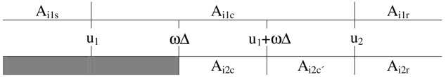
Figure 1: Structure of the adopted GDCE model (not to scale). $A_{i}$ is the abundance of element $i$. The indices 1 and 2 represent the prompt and delayed contributions, respectively. The indices $s$, $c$, $c^{\prime}$, and $r$ are relative to the simple model ($s$), Clayton model with delayed production contribution from stars born during the simple model phase ($c$) and after the start of infall ($c^{\prime}$), and ISM dilution due to effect of refuse ($r$).

Eu evolution is modeled by the same formulation used for Fe. Th requires specific formulation due to its radioactive decay. Another important phenomenon, besides radioactive decay, must be taken into consideration when modeling Th evolution: selective destruction by photonuclear reactions in the stellar interior (Malaney et al. 1989). During H burning via the CN cycle, 7.29 MeV and 7.55 MeV $\gamma$ photons are emitted. These photons have energies below the photonuclear threshold of most elements existing in stellar interiors, including Fe and Eu. However, Th has a threshold of $\sim 6\leavevmode\nobreak\ \mbox{MeV}$, which allows the destruction of up to $\sim 40\%$ of its initial content in a stellar core. When the star evolves to become a red giant, the first dredge-up takes Th-depleted matter from the stellar interior to the photosphere. Matter ejected at the end of stellar evolution has a reduction in Th abundance of $\sim 10\%\mbox{--}20\%$. This phenomenon is properly considered in Arany-Prado & Maciel (1998, APM98), following Malaney et al. (1989). The general equation for the abundance $A_{i}$ is

$$\frac{\mathrm{d}(gA_{i})}{\mathrm{d}u}+(J_{1}+J_{2})gA_{i}=P_{i},$$ (3)

where

$$J_{1}=\left\{\begin{array}[]{l @{ \quad} l l}1,&\mbox{for }u&<u_{2},\\ 1+\Gamma,&\mbox{for }u&\geq u_{2},\end{array}\right.$$ (4)

$$J_{2}=\left\{\begin{array}[]{l @{ \quad} l l}0,&\mbox{for stable elements,}\\ \frac{\lambda_{i}}{\omega}+\Lambda_{i},&\mbox{for r-process radionuclides,}\end{array}\right.$$ (5)

$$P_{i}=\left\{\begin{array}[]{l l @{ \quad} l l}p^{i}_{1}g(u),&&\mbox{for }u&<\omega\Delta,\mbox{\ or for}\\ &&\mbox{prompt-enrichment}&\\ &&\mbox{elements},\mbox{and}&\\ p^{i}_{1}g(u)+p^{i}_{2}g(u-\omega\Delta),&&\mbox{for }u&\geq\omega\Delta.\end{array}\right.$$ (6)

$\lambda_{i}$ is the decay constant and $\Lambda_{i}$ is the destruction term (APM98, Eq. 9) of element $i$; $p^{i}_{1}$ and $p^{i}_{2}$ are the net yields of element $i$, as defined by Eq. 8 of APM98 (as well as by Eqs. 6 and 7 of PT95); the indices 1 and 2 refer to the prompt and delayed contributions, respectively.

2.1.2 Observational constraints and adopted constants

Calculations were carried out for four Galactic disk ages: 6, 9, 12, and 15 Gyr. Parameter $u_{1}$ was kept at the value assumed by PT95 (0.14). The delay $\Delta$ was fixed at 1.1 Gyr both for Fe and for Eu; this value is consistent with the average evolution timescales of progenitors of Type Ia supernovae (which are the main astrophysical sites of Fe production) and asymptotic giant branch stars (which are the sites of s-process Eu production). Note that delayed production of Eu is properly accounted for in this work, but that its effects are nonetheless small, since Eu is majorly (97%, according to Burris et al. 2000) synthesized by the r-process.

We adopted the initial mass function (IMF) of Kroupa (2001, Eq. 6), which covers non-stellar masses (brown dwarfs) down to $0.010\leavevmode\nobreak\ m_{\mbox{\scriptsize\sun}}$. We extended this lower segment down to $0.001\leavevmode\nobreak\ m_{\mbox{\scriptsize\sun}}$, keeping the same slope, and included a new segment corresponding to the residues that evaporate, with a slope $j$ which is a free model parameter. The complete IMF was defined as follows:

$$\Phi(m)=\left\{\begin{array}[]{l @{, \quad} l l}a_{1}\,m^{-j}&\mbox{for }0.000&\lesssim m/m_{\mbox{\scriptsize\sun}}\leq\mathrm{\ \ }0.001;\\ a_{2}\,m^{-0.3}&\mbox{for }0.001&<m/m_{\mbox{\scriptsize\sun}}\leq\mathrm{\ \ }0.080;\\ a_{3}\,m^{-1.8}&\mbox{for\ }0.080&<m/m_{\mbox{\scriptsize\sun}}\leq\mathrm{\ \ }0.500;\\ a_{4}\,m^{-2.7}&\mbox{for }0.500&<m/m_{\mbox{\scriptsize\sun}}\leq\mathrm{\ \ }1.000;\\ a_{5}\,m^{-2.3}&\mbox{for }1.000&<m/m_{\mbox{\scriptsize\sun}}\leq 62.000.\end{array}\right.$$ (7)

It is worth noting that the IMF for the residues relates to the mass of residues prior to evaporation. If the IMF from Miller & Scalo (1979) had been used, the slope of the residues mass range would have to be steeper to compensate for the decrease at low mass range, maintaining normalisation. The sudden change of slope between residue and brown dwarf ranges would be harder to explain than the slower, more continuous increase that can be achieved when using Kroupa’s IMF. The same would occur if we adopted the IMF from Salpeter (1955).

The parameters $\omega$ and $u_{0}$ were evaluated for different values of $k$ and for each Galactic disk age, so that at $T_{\mathrm{G}}$ we have $\mu$ = present-day gas fraction = 0.11 and $g$ = mass of gas ${\sim(0.73\,\mbox{initial disk mass})}$, as considered by PT95. For a given set of values of the parameters $k$, $\omega$, $u_{o}$, and T_G, we fitted the metallicity distribution of G dwarfs obtained from the model to the observational distribution of Rocha-Pinto & Maciel (1996). The fitting was accomplished by changing the parameter $j$ and, consequently, the parameter $\Gamma$, since the Jovian planet and residue formation rate is given by $\int_{0}^{0.010}m\Phi(m)\,\mathrm{d}m$ (cf. Equations 2 and 7). For a given value of parameter $j$, parameters $a_{1}$, $a_{2}$, $a_{3}$, $a_{4}$, and $a_{5}$ (Equation 7) were obtained by enforcing IMF continuity and normalisation. The best values of $j$ (2.562–2.605) are similar to the IMF slopes for the ranges of stellar masses that would form planets $(2.7\mbox{\ for\ }0.5<m/m_{\mbox{\scriptsize\sun}}\leq 1.0\mbox{\ and\ }2.3\mbox{\ for\ }1.0<m/m_{\mbox{\scriptsize\sun}}\leq 62.0)$, which implies that equal masses form stars and residues – see Table 2. In this table, $f_{1}=p_{1}/A_{\mbox{\scriptsize\sun}}$ and $f_{2}=p_{2}/A_{\mbox{\scriptsize\sun}}$.

Good fits were found for $k=2$ and $k=3$; we adopted $k=2$, because this value provides a better fit to the four Galactic disk ages simultaneously. This lends support to the hypothesis that the effect of refuse can substitute for the dilution caused by infall at later stages of Galactic evolution, since PT95 manage to obtain good fits only with $k=3$. The final metallicity distributions of G dwarfs obtained from the model are compared to Rocha-Pinto & Maciel (1996) in Fig. 2.

Figure 2: Metallicity distribution of G dwarfs in the solar neighbourhood, where $\Delta\mathrm{N}/\mathrm{N}$ is the normalised number of stars. The thick curve is the observational distribution of Rocha-Pinto & Maciel (1996). The thin curves were calculated using our GDCE model for the four different Galactic disk ages shown in the legend.

For the modeling of Eu and Th evolutions, the relevant parameters are their respective $f_{1}$ and $f_{2}$. For Eu, the total value $f_{\mathrm{total\,Eu}}$, which takes prompt and delayed production into consideration, was determined by fitting the [Eu/Fe] vs. [Fe/H] curve obtained from the calculations to our stellar data (Table 14 of Paper I). We assumed that prompt production of Eu is accomplished by the r-process, while delayed production is carried out by the s-process (with relative contributions 0.97 and 0.03, respectively, according to Burris et al. 2000), leading to $f_{1\,\mathrm{Eu}}=0.97\,f_{\mathrm{total\,Eu}}$ and $f_{2\,\mathrm{Eu}}=0.03\,f_{\mathrm{total\,Eu}}$. Th is synthesized exclusively by the r-process and its production was considered proportional to the production of Eu: $f_{1\,\mathrm{Th}}=\chi\,f_{\mathrm{total\,Eu}}$ and $f_{2\,\mathrm{Th}}=0$. The parameter $\chi$ used was the one that provided the best simultaneous fit of the [Th/H], [Th/Fe], and [Th/Eu] vs. [Fe/H] curves, obtained by the model, to our stellar data. Table 1 provides summarised descriptions of the main GDCE model parameters, and the final values adopted are listed in Table 2, as a function of Galactic disk age.

Table 1: Summarised descriptions of the main GDCE model parameters.

Parameter	Short description
$k$	Small positive integer used to parametrize the mass
	infall rate $F$.
$\Delta$	Time after the start of stellar formation, after which
	delayed-production elements start being ejected.
$\omega$	Efficiency of interstellar gas conversion into stars.
$u_{0}$	Arbitrary parameter in the mass infall rate $F$.
$u_{1}$	Time of transition between simple and Clayton
	model, multiplied by $\omega$.
$u_{2}$	Time when residue formation becomes efficient,
	multiplied by $\omega$.
$u_{T_{\mathrm{G}}}$	Age of the Galactic disk, multiplied by $\omega$.
$j$	IMF slope corresponding to residues that evaporate.
$\Gamma$	Dilution of ISM due to residue evaporation.
$f_{1\,\mathrm{Fe}}$	Fe yield divided by Fe solar abundance today
	(prompt contribution).
$f_{2\,\mathrm{Fe}}$	Fe yield divided by Fe solar abundance today
	(delayed contribution).
$f_{\mathrm{total\,Eu}}$	Eu yield divided by Eu solar abundance today.
$f_{1\,\mathrm{Eu}}$	Prompt contribution of $f_{\mathrm{total\,Eu}}$.
$f_{2\,\mathrm{Eu}}$	Delayed contribution of $f_{\mathrm{total\,Eu}}$.
$f_{1\,\mathrm{Th}}$	Th yield divided by Th solar abundance today.
$\chi$	Relation between $f_{1\,\mathrm{Th}}$ and $f_{\mathrm{total\,Eu}}$.

Table 2: Adopted GDCE model parameters. For a short description of the entries, see Table 1; details can be found in the text.

	$T_{\mathrm{G}}$
Parameter	6 Gyr	9 Gyr	12 Gyr	15 Gyr
$k$	—————–  2  ——————-
$\Delta$ (Gyr)	—————–  1.1  ——————
$\omega$	0.746	0.488	0.362	0.285
$u_{0}$	2.040	1.500	1.250	1.110
$u_{1}$	—————-  0.140  —————-
$u_{2}$	1.880	1.845	1.824	1.796
$u_{T_{\mathrm{G}}}$	4.476	4.392	4.344	4.275
$j$	2.605	2.586	2.571	2.562
$\Gamma$	0.301	0.251	0.217	0.199
$f_{1\,\mathrm{Fe}}$	—————-  0.240  —————-
$f_{2\,\mathrm{Fe}}$	—————-  0.467  —————-
$f_{\mathrm{total\,Eu}}$	0.630	0.670	0.710	0.750
$f_{1\,\mathrm{Eu}}$	0.611	0.650	0.689	0.728
$f_{2\,\mathrm{Eu}}$	0.019	0.020	0.021	0.022
$f_{1\,\mathrm{Th}}$	0.740	0.905	1.186	1.425
$\chi$	1.175	1.350	1.670	1.900

Observations:	$u_{T_{\mathrm{G}}}=\omega\,T_{\mathrm{G}}$; $f_{1\,\mathrm{Eu}}=0.97\,f_{\mathrm{total\,Eu}}$;
	$f_{2\,\mathrm{Eu}}=0.03\,f_{\mathrm{total\,Eu}}$; $f_{1\,\mathrm{Th}}=\chi\,f_{\mathrm{total\,Eu}}$.

2.2 The age of the Galactic disk

We have estimated the age of the Galactic disk in two different ways: using our GDCE model along with literature production ratio data, and with our own stellar abundance data.

2.2.1 $T_{\mathrm{G}}$ from literature data

Inspection of Table 2 shows that parameter $\chi$ is not constant, but dependent on the Galactic disk age. Therefore, the age can be estimated by constructing a $\chi$ vs. $T_{\mathrm{G}}$ diagram, fitting a curve to the diagram to determine a relation between the two parameters, and then using literature determinations of $\chi$. Parameter $\chi$ can be calculated from literature determinations of solar Eu and Th abundances and Th/Eu production ratio through the relation $\chi=(p^{\mathrm{Th}}/p^{\mathrm{Eu}})/(\mbox{Th}/\mbox{Eu})_{\mbox{\scriptsize\sun}}$, where $(\mbox{Th}/\mbox{Eu})_{\mbox{\scriptsize\sun}}$ is the solar abundance ratio today.

From the meteoritic determinations originally presented by Lodders (2003) we have $\log\varepsilon(\mbox{Th})_{\mbox{\scriptsize\sun}}=+0.06\pm 0.04$ and $\log\varepsilon(\mbox{Eu})_{\mbox{\scriptsize\sun}}=+0.49\pm 0.04$, which leads to $(\mbox{Th}/\mbox{Eu})_{\mbox{\scriptsize\sun}}=+0.372\pm 0.069$. These abundances were not taken directly from Lodders (2003), but rather from Asplund et al. (2005), who corrected their zero-point in order to make them compatible with their Si photospheric value. It is much more difficult to estimate the production ratio $p^{\mathrm{Th}}/p^{\mathrm{Eu}}$. Some of the works from the literature that estimate the ages of UMP stars through Th/Eu nucleocosmochronology use the solar Th/Eu abundance ratio, corrected for the Th decay since the formation of the Sun, as an estimate of the production ratio. This approach would lead to a good estimate only if all solar Th were produced in a single (or at most a few) nucleosynthesis episodes just prior to the formation of the Solar System. This hypothesis is known to be false, and stellar ages estimated with production ratios obtained this way yield lower limits only. For this reason, it is preferable to use theoretical estimates.

Theoretical production ratios are derived from models of r-process nucleosynthesis, and subject to many uncertainties, mainly because the astrophysical site of production by this process is not well known yet, and because it is not possible to obtain laboratory data on many very-neutron-rich elements which are very far from the $\beta$-stability valley. A procedure frequently employed to reduce these uncertainties is to constrain the model results to solar abundances. Heavy elements currently present in the Sun have been synthesized by both the r-process and s-process (with the exception of U and Th, produced exclusively by the r-process). R-process nucleosynthesis models are then forced to reproduce just the fraction of the solar abundances that was produced by the r-process. This constraint is valid only if all stars produce r-process elements in solar proportions. The abundances of heavy elements in UMP stars could also be used to constrain the r-process nucleosynthesis models, but their high uncertainty makes it preferable to use the solar abundances.

Many works from the literature (Sneden et al. 1996, 1998, 2000a, 2000b; Westin et al. 2000; Burris et al. 2000; Johnson & Bolte 2001; Cowan et al. 1999, 2002, among others) corroborate the so-called universality of the r-process abundances. According to this hypothesis, r-process nucleosynthesis would occur at only one astrophysical site and would always produce elements in solar proportions. These works support the universality hypothesis by the successful comparison of heavy element abundances in UMP stars (representing the product of nucleosynthesis from few preceding stars) with r-process fraction of solar abundances (representing the cumulative production during several Gyr of Galactic evolution). This comparison is carried out for the second and third r-process peaks only ($56\leq\mbox{Z}\leq 72$ and $73\leq\mbox{Z}\leq 82$, respectively). To enable the use of r-process nucleosynthesis models which are constrained to solar abundances in the calculation of Th/Eu production ratios, Th must also be included in the universality. It is usually assumed that, if the universality is valid for second and third peaks, it can be extended to the actinides. Determination of more precise Pb and Bi abundances in the Sun and UMP stars would allow us to better investigate if this extension is indeed valid or not. Since these elements are produced mainly (more than 80%) by the $\alpha$-decay of elements with atomic mass $209<\mbox{A}<255$, it would be very unlikely that solar Pb and Bi abundances would be compatible with those from UMP stars if universality was not valid for elements with $\mbox{A}>209$.

The supposition that universality can be extended to the actinides is still a matter of strong polemic in the literature. In particular, the analyses of the halo UMP giant CS 31 082-001 carried out by Cayrel et al. (2001) and Hill et al. (2002) provide data against it. This star presents a solar abundance pattern for elements of the second peak, but its third peak does not match the Sun. While Os and Ir seem to be overabundant relative to the solar r-process fraction, Pb appears to be deficient. A more significant discrepancy is that the star has an abundance ratio $\mbox{Th/Eu}=+0.603$, which is much larger than the solar value corrected for Th decay $\mbox{(Th/Eu)}_{\mbox{\scriptsize\sun}}=+0.434$; UMP stars are expected to present Th/Eu abundance ratios considerably lower than the solar corrected value, due to their higher age. This high value indicates that the star could have been formed with an inherent actinide superabundance relative to the elements of the second peak, which means that universality would not hold for Th. CS 31 082-001 is the only star hitherto studied that presents important discrepancies for elements with $\mbox{Z}>55$, whereas evidence favorable for the validity of universality for these atomic masses is becoming increasingly numerous. It is not clear if CS 31 082-001 is merely chemically peculiar or if its discrepancies could be present in other yet unobserved stars; if the latter is true, it may not be possible to extend universality to the actinides. If Eu and Th are produced in different astrophysical sites, the Th/Eu production ratio may have suffered variations during the evolution of the Galaxy, provoked by changes in the relative frequencies of their respective progenitors.

In this paper, we assume that universality can be extended to Th, considering that indications to the contrary are very sparse. But even if constraining the nucleosynthesis models to solar abundances reduces the uncertainties, they nevertheless remain very high, because the calculations can be based on different far-from-stability mass models and other theoretical suppositions (e.g., neutron densities). Cowan et al. (1997, 1999) and Schatz et al. (2002) derive values between 0.47 and 0.55. We adopted the center of the interval, $p^{\mathrm{Th}}/p^{\mathrm{Eu}}=0.51\pm 0.04$, arriving at $\chi=1.371^{+0.444}_{-0.305}$. In Fig. 3 the $T_{\mathrm{G}}$ vs. $\chi$ diagram constructed for our GDCE model is presented. A linear fit to the data was used to estimate a Galactic disk age of $T_{\mathrm{G}}=8.7^{+5.3}_{-3.6}\leavevmode\nobreak\ \mbox{Gyr}$. Taking into account the linear fit scatter ($\sigma=0.5$), we arrive at a final value $T_{\mathrm{G}}=8.7^{+5.8}_{-4.1}\leavevmode\nobreak\ \mbox{Gyr}$. The high uncertainty of this result reflects the difficulties of estimating the Th/Eu production and solar abundance ratios, as well as the low sensitivity of the Galactic disk age to parameter $\chi$.

Figure 3: $T_{\mathrm{G}}$ vs. $\chi$ diagram for our GDCE model. The dotted curve is a linear fit. The solid lines display the value adopted from the literature for the $\chi$ parameter ($1.371^{+0.444}_{-0.305}$) and its respective disk age ($8.7^{+5.3}_{-3.6}\leavevmode\nobreak\ \mbox{Gyr}$).

2.2.2 $T_{\mathrm{G}}$ from our stellar data

[Th/Eu] vs. [Fe/H] curves were constructed from our GDCE model for each Galactic disk age. These curves, along with our stellar abundance ratio data, can be seen in Fig. 4. Note that the curves draw further apart at high metallicities. This has a very important consequence for the analysis: contrary to the intuitive notion that the most metal-poor stars are the most important, it is the most metal-rich ones which better discriminate between different ages. In order to determine the age that best fits our data, we calculated a quadratic deviation between our data points and each curve, according to the equation

$$\mbox{Total deviation}=\sum_{i=1}^{19}\left\{[\mbox{Th/Eu}]_{i}-f([\mbox{Fe/H}]_{i})\right\}^{2},$$ (8)

where the index $i$ represents the $i$-th star, and $f([\mbox{Fe/H}]_{i})$ is a $4^{\mathrm{th}}$ order polynomial fit to the GDCE curve. We were not able to use all 21 sample stars to calculate the deviations because the two most metal-rich objects (HD~128 620 and HD~160 691) fall out of the interval where the curves are defined; that is why the total deviations were calculated by summing 19 individual stellar deviations, and not 21.

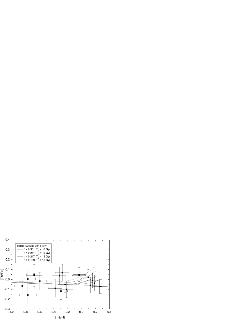
Figure 4: [Th/Eu] vs. [Fe/H] diagram for all sample stars. Curves were calculated using our GDCE model for the four different Galactic disk ages shown in the legend.

Once a deviation was determined for each curve, we traced a deviation vs. $T_{\mathrm{G}}$ diagram, and fitted a $2^{\mathrm{nd}}$ order polynomial to it (Fig. 5). The Galactic disk age that best fits our stellar [Th/Eu] abundance ratio data was obtained by minimising the fitted polynomial: $T_{\mathrm{G}}=8.2\leavevmode\nobreak\ \mbox{Gyr}$.

Figure 5: Determination of Galactic disk age that best fits our stellar [Th/Eu] abundance ratio data. Points are the total deviations between each curve and the stellar data presented in Fig. 4, calculated according to Equation 8. The curve is a $2^{\mathrm{nd}}$ order polynomial fit. The vertical line marks the polynomial minimum, corresponding to best Galactic disk age $T_{\mathrm{G}}=8.2\leavevmode\nobreak\ \mbox{Gyr}$.

We estimated the Galactic disk age uncertainty related to the abundance ratio uncertainties by Monte Carlo simulation. We developed a code that adds Gaussian random errors to the stellar [Th/Eu] and [Fe/H] abundance ratios, where the width of the Gaussians are the uncertainties adopted for the respective abundance ratio. After this, the code calculates the new total deviations between the GDCE curves and the modified stellar data, fits a $2^{\mathrm{nd}}$ order polynomial to the [deviation, $T_{\mathrm{G}}$] data, and calculates the polynomial minimum, obtaining a new age. It is possible to choose the number of simulations, each time with new abundance ratios, added to different Gaussian errors. The ages obtained are saved in a file for further analysis.

We carried out 75 million simulations. The Galactic disk age distribution obtained is presented in Fig. 6, where ages were counted in 0.5 Gyr bins. The few negative ages obtained ($<0.2\%$) were removed, since they make no physical sense. The distribution has a clear increase in noise as the age increases (after the mode). This happens because the distribution was constructed by counting the number of ages between two values. Thus, as the age increases, the number of counts decreases, and statistical fluctuation increases. Because of this, we truncated the distribution at 125 Gyr, where the counts drop below 100 (corresponding to a 10% statistical uncertainty). One other issue, besides the noise, forced us to truncate the distribution at a point where the counts are still statistically significant. A continuous probability distribution must fall asymptotically to zero. But this cannot occur with our distribution, as it was constructed by counting, and counts have no fractional values between 0 and 1. Hence, the result of the calculations performed to derive an age uncertainty would be incorrect if we took into consideration the complete distribution.

Figure 6: Galactic disk age distribution obtained through a Monte Carlo simulation of the [Th/Eu] and [Fe/H] abundance ratio uncertainties. Simulation results have been counted in 0.5 Gyr bins, and N is the total count per bin. The vertical line marks the age at which the distribution was cut (125 Gyr), corresponding to a count fall below 100 (i.e., 10% uncertainty).

A good estimate for our age uncertainty is the width of the distribution. There is more than one way to estimate this width. The most widely used is the variance, determined through the equation

$$\sigma^{2}=\int_{0}^{125}\frac{N}{N_{\mathrm{total}}}(T_{\mathrm{G}}-\overline{T}_{\mathrm{G}})^{2}\,\mbox{d}T_{\mathrm{G}},$$ (9)

where $N_{\mathrm{total}}$ is the total number of simulations within the integration limits and $\overline{T}_{\mathrm{G}}$ is the average age. The integration limits should have been $-\infty$ and $+\infty$, but since the distribution was truncated at 0 and 125, we carried out the integration accordingly. In Fig. 7 the integrand of Equation 9 is presented, and it can be seen that its right wing falls very slowly. Even if we extended the upper integration limit to $+\infty$, it is possible that convergence could not be achieved. Even if we managed to achieve convergence, the value obtained would be very large, and not representative of the width of the distribution.

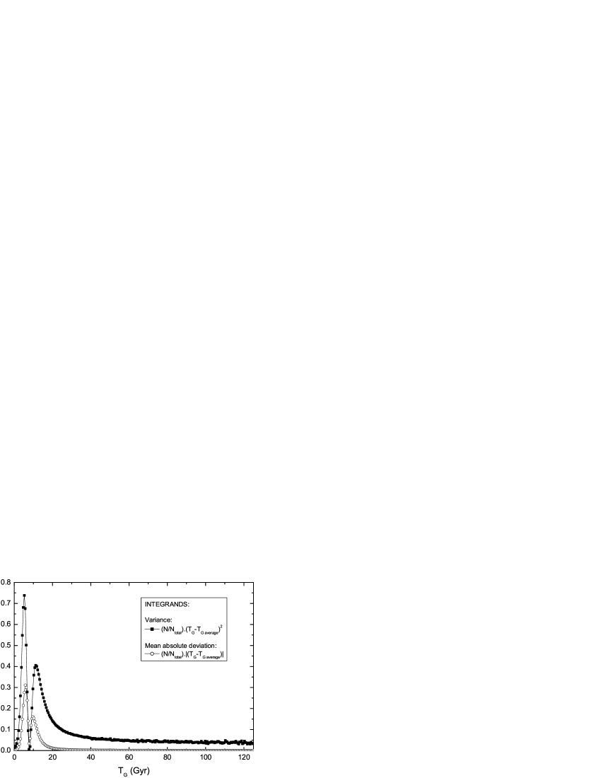
Figure 7: Integrands of Equations 9 and 10, used to calculate the variance and the mean absolute deviation (MAbD) of the age distribution, respectively.

A more robust estimator of the width is the mean absolute deviation (MAbD, see Press et al. 1992):

$$\mbox{MAbD}=\int_{0}^{125}\frac{N}{N_{\mathrm{total}}}|T_{\mathrm{G}}-\overline{T}_{\mathrm{G}}|\,\mbox{d}T_{\mathrm{G}}.$$ (10)

As can be seen in Fig. 7, the integrand of Equation 10 falls to zero much faster than that of Equation 9. Therefore, the integration converges, and the error introduced by truncating the distribution can be neglected. Carrying out a numeric integration, we arrive at $\mbox{MAbD}=1.9\leavevmode\nobreak\ \mbox{Gyr}$. The procedure was repeated several times, with different bin sizes, and we verified that the MAbD is not dependent on the bin size.

The final value obtained using our stellar data is $T_{\mathrm{G}}=(8.2\pm 1.9)\leavevmode\nobreak\ \mbox{Gyr}$. It must be noted that the cited uncertainty is related to the stellar [Th/Eu] and [Fe/H] abundance ratio uncertainties alone, and does not take into consideration the uncertainties of the GDCE model itself, which are very difficult to estimate. The uncertainty related to the model could very well be the main source of age uncertainty.

2.2.3 Adopted Galactic thin disk age

The adopted Galactic disk age was calculated by combining the two estimates obtained with literature data and with our stellar abundance ratios. These values were combined using the maximum likelihood method, assuming that each one follows a Gaussian probability distribution, which results in a weighted average using the reciprocal of the square uncertainties as weights. The final, adopted Galactic disk age is

$$\mbox{FINAL }T_{\mathrm{G}}=(8.3\pm 1.8)\leavevmode\nobreak\ \mbox{Gyr.}$$

3 Conclusions

[Th/Eu] vs. [Fe/H] curves have been constructed for four Galactic disk ages (6, 9, 12, and 15 Gyr) from a GDCE model developed by us. These curves were compared to the stellar abundance ratio data obtained in Paper I in order to determine the Galactic disk age. The age that best fits our data was obtained by minimising the total quadratic deviation between the stellar data and the theoretical curves. A Monte Carlo simulation was carried out to estimate the age uncertainty related to the abundance ratio uncertainties. The value obtained was $T_{\mathrm{G}}=(8.2\pm 1.9)\leavevmode\nobreak\ \mbox{Gyr}$. The age was also estimated using literature data along with our GDCE model, yielding $T_{\mathrm{G}}=8.7^{+5.8}_{-4.1}\leavevmode\nobreak\ \mbox{Gyr}$.

Our two age estimates were combined using the maximum likelihood method, resulting in $\mbox{FINAL }T_{\mathrm{G}}=(8.3\pm 1.8)\leavevmode\nobreak\ \mbox{Gyr}$. This result is the first Galactic disk age determined via Th/Eu nucleocosmochronology, and is compatible with the most recent white dwarf ages determined via cooling sequence calculations, which indicate a low age ($\lesssim 10\leavevmode\nobreak\ \mbox{Gyr}$) for the disk (Oswalt et al. 1995; Bergeron et al. 1997; Leggett et al. 1998; Knox et al. 1999; Hansen et al. 2002).

Determination of the Galactic disk age via [Th/Eu] nucleocosmochronology was found to be very sensitive to observational uncertainties. The GDCE model is very insensitive to the choice of disk age, and the curves derived from the model are very close when compared to the abundance uncertainties. This leads to an age uncertainty as high as 1.9 Gyr relative to the abundance ratio uncertainties alone, not taking into account the uncertainties intrinsic to the GDCE model itself, which are very difficult to evaluate. The analysis performed with production ratios and solar abundances taken from the literature presents an even higher uncertainty. However, considering that we managed to reduce the Eu and Th abundance scatters significantly, when compared to the best data currently available in the literature, we believe that additional improvements may raise the precision of the analysis even further. Among the possible enhancements, we can cite the observation of higher resolution, higher S/N ratio spectra (preferentially with large sized telescopes), determination of higher precision atomic parameters (e.g., central wavelengths of absorption lines), and identification of yet unknown line blends, like those that forced us to include artificial Fe lines in the spectral syntheses. If part of the data scatter is real, and not observational, it will not be possible to reduce it indefinitely. This may be true if the Th/Eu production ratio is not constant throughout the Galactic evolution, as abundance analyses of r-process elements in CS 31 082-001 seem to indicate. Future advancements in r-process nucleosynthesis models may help solve the issues of universality and constancy of the production ratio, especially when the sites of production by this process are finally identified.