Illuminating Dark Energy with Cosmic Shear

Abstract

One of the principal goals of modern cosmology is to constrain the properties of dark energy. At present, numerous surveys are aiming to determine the equation of state, which is assumed constant due to our poor understanding of its behaviour (and since higher order parameterisations lead to unwieldy errors). This raises the question - how does our “best-fit” equation of state relate to the true function, which may vary with redshift. Saini et al. (2003) Deep Saini et al. (2003) have demonstrated that the value of $w$ attained by a supernovae study is well described by a weighted integral over the true function. Adopting a similar approach, we calculate the corresponding “weight function” for a fiducial cosmic shear survey. We disentangle contributions from the angular diameter distance and the growth factor, finding that they partially cancel each other out. Consequentially, the sensitivity to $w$ at high redshift is enhanced beyond that of supernovae studies, and is comparable, if not higher, than lensing of the CMB. This illustrates the complementary nature of the different techniques. Furthermore, we find that results which would naïvely be interpreted as inconsistent could arise from a time-dependent equation of state.

I Introduction

Following the rapid accumulation of experimental evidence Perlmutter et al. (1999); Allen et al. (2004); Tegmark et al. (2004); Spergel et al. (2003), it has become generally accepted that the universe is presently experiencing a period of accelerated expansion. In the context of general relativity, this implies that current cosmological dynamics are dominated by a component with negative pressure. By revealing the behaviour of this dark energy, not only might we foresee the ultimate fate of the universe, but this may be the first step into a new field of physics.

The equation of state for dark energy, defined as the pressure to density ratio $w=p/\rho$, provides us with an observable quantity which may differentiate between the leading candidates. Any deviation from $w=-1$ (the value indicative of the cosmological constant) imparts two major influences in cosmology. For a fixed dark energy density, a more negative $w$ is associated with stronger pressure, which in turn enhances the expansion of the universe.

The effect of this can be seen in cosmography (measurements of the global properties of the universe), such as luminosity distance (in the case of supernovae), and comoving angular diameter distance (in the case of weak lensing).

Secondly, the dark energy density evolution is governed by $w$. A more negative $w$ leads to the mass fraction of dark energy $\Omega_{\rm DE}$ decaying more rapidly with redshift. This alters both the expansion and structure formation histories.

The results of dark energy studies may be concisely expressed as an array of estimated values for the (constant) equation of state. It is imperative that we are alert to the various interpretations which may be drawn from this, bearing in mind the possibility that $w$ is time-dependent. In this study we will concentrate on the redshift sensitivity with which cosmic shear probes dark energy, and the extent to which the data complements that of supernovae surveys.

Cosmic shear is perhaps the most promising technique for quantifying dark energy, largely due to the simplicity of the underlying physics.

Apparent alignments of distant galaxies arise from weak gravitational lensing by intervening structure Van Waerbeke et al. (2000); Bacon et al. (2000); Wittman et al. (2000); Jarvis et al. (2003); Kaiser et al. (2000). The strengths of these correlations are dictated by two cosmological features: the matter power spectrum, and the lens geometry. In turn, both of these depend on $w$. Here we study their relative contributions to the shear signal, and show how this influences the range of $w(z)$ to which cosmic shear is most sensitive.

The structure of this article is as follows. In §II the theory of cosmic shear is briefly reviewed, along with the approach we will use to evaluate the weight function.

We present the weight function for a fiducial cosmic shear survey in §III, separating its contributions from the geometry and the growth of structure. This is extended in §IV to tomography, while §V uses an alternative method to investigate whether cosmic shear measures $w$ via its influence on structure growth or the expansion rate. Lensing of the cosmic microwave background and cosmic shear surveys by the Large Synoptic Survey Telescope (LSST) and Canada-France-Hawaii Telescope Legacy Survey (CFHTLS) are considered in §VI. Finally, we compare the information which can be extracted from lensing and supernova surveys in §VII.

II The Sensitivity of Cosmic Shear

Here we relate the underlying equation of state $w(z)$ to the constant value $w$ which provides the best fit to cosmic shear data. The survey parameters used are that of the proposed Supernovae/Acceleration Probe (SNAP), although as we shall see in §VI our results are robust to the exact specifications, with the exception of the survey depth.

II.1 Methodology

II.1.1 The Matter Power Spectrum

We adopt the following $\Lambda$CDM cosmology as our fiducial model: $w=-1$, $\Omega_{m}=0.3$, spectral index $n=1$, baryon fraction $\Omega_{b}=0.047$, $\sigma_{8}=0.88$, and Hubble parameter $h=0.7$.

To produce the matter power spectrum $P(k,z)$ we use the shape parameter of Sugiyama $[\Gamma=\Omega_{m}h\exp[-\Omega_{b}(1+\sqrt{2h}/\Omega_{m})]]$. Linear growth of structure is evaluated in accordance with standard theory:

$$\ddot{\delta}_{m}+\frac{3}{2a}\big{[}1-w(a)(1-\Omega_{m}(a))\big{]}\dot{\delta}_{m}-\frac{3}{2a^{2}}\Omega_{m}(a)\delta_{m}=0.$$ (1)

For this study the large-scale clustering of dark energy is considered to be of little significance Ma et al. (1999). We then apply the fitting formula from Peacock & Dodds Peacock and Dodds (1996), whilst acknowledging that a more sophisticated approach would be preferred when modelling quintessence cosmologies.

II.1.2 Weak Lensing

The shear power spectrum is given by

$$C_{\ell}=\frac{\displaystyle 9}{16}\Big{(}\frac{\displaystyle H_{0}}{\displaystyle c}\Big{)}^{4}\Omega_{m}^{2}\int^{\chi}_{0}\Big{[}\frac{\displaystyle g(\chi)}{\displaystyle ar(\chi)}\Big{]}^{2}P(\frac{\ell}{r},\chi)\mathrm{d}\chi$$ (2)

where $\chi$ is the coordinate distance, and $r(\chi)$ the comoving angular diameter distance. We assume a flat universe throughout, and thus $r(\chi)=\chi$. $P(\ell/r,\chi)$ is the matter power spectrum for wavenumber $\ell/r$ at a redshift corresponding to a coordinate distance $\chi$. The lensing efficiency term $g(\chi)$ favours the density perturbations which are approximately equidistant from the source and observer:

$$g(\chi)=2\int_{\chi}^{\chi_{h}}n(\chi^{\prime})\frac{r(\chi)r(\chi^{\prime}-\chi)}{r(\chi^{\prime})}\mathrm{d}\chi^{\prime},$$ (3)

where $n(\chi)$ is the galaxy probability density function, with respect to comoving distance (see Bartelmann & Schneider Bartelmann and Schneider (1999) and Mellier Mellier (1999) for reviews).

Multipole errors are, in accordance with Kaiser Kaiser (1998), given by

$$\sigma(\ell)=\sqrt{\frac{\displaystyle 2}{\displaystyle(2\ell+1)f_{sky}}}(C_{\ell}+\frac{\displaystyle\sigma^{2}_{\gamma}}{\displaystyle 2n_{g}}),$$ (4)

where $f_{sky}$ is the area expressed as a fraction of the whole sky, $n_{g}$ is the number of galaxies per steradian and $\sigma_{\gamma}$ is the rms intrinsic (pre-lensing) ellipticity of the galaxies in the sample.

For the purposes of our calculations we followed the fitting function and survey parameters from Refregier et al. Refregier et al. (2004)

$$n(z)\propto z^{\alpha}e^{-(z/z_{0})^{\beta}}.$$ (5)

For simulating the SNAP wide survey the following figures were used: redshift parameter $z_{0}=1.13$, $\alpha=2$, $\beta=2$, $f_{sky}$ is the equivalent of $1000$ square degrees, $n_{g}=100$ ${\rm arcmin}^{-2}$ and $\sigma_{\gamma}=0.31$.

In light of an investigation by Cooray & Hu Cooray and Hu (2001), we can afford to ignore the correlation of errors for different $\ell$’s. Furthermore, we enforce an upper limit of $\ell<10^{4}$, above which the baryons are considered to introduce a significant uncertainty in the power spectrum estimation White (2004); Zhan and Knox (2004). At the end of § III.2 we investigate the effect of adopting a more conservative upper limit.

II.2 Response to the Equation of State

The functional derivative describes the manner in which the shear signal reacts to changes in the value of $w$ at various redshifts

$$\frac{\partial C_{\ell}(w^{\rm fid})}{\partial w(z)}\Bigg{\arrowvert}_{z^{\prime}}=\lim_{\epsilon\rightarrow 0}\frac{C_{\ell}(w^{\rm fid}+\epsilon\delta(z-z^{\prime}))-C_{\ell}(w^{\rm fid})}{\epsilon}.$$ (6)

Since $w$ only imparts a small change in the observed shear, we can approximate the deviation from a fiducial model as

$$C_{\ell}\simeq C_{\ell}(w^{\rm fid})+\int{\frac{\partial C_{\ell}(w^{\rm fid})}{\partial w(z)}\Bigg{\arrowvert}_{z^{\prime}}(w(z^{\prime})-w^{\rm fid}(z^{\prime}))\mathrm{d}z^{\prime}}.$$ (7)

Before proceeding further we introduce the notation $\delta w(z^{\prime})=w(z^{\prime})-w^{\rm fid}(z^{\prime})$, $\Delta w=w^{\rm fit}-w^{\rm fid}$, and $K(\ell,z^{\prime})=\partial C_{\ell}(w^{\rm fid})/\partial w(z)$. Therefore

$$C_{\ell} \simeq C_{\ell}(w^{fid})+\int{K(\ell,z^{\prime})\delta w(z^{\prime})\mathrm{d}z^{\prime}}$$ (8)

$$C^{fit}_{\ell} \simeq C_{\ell}(w^{fid})+\Delta w\int{K(\ell,z^{\prime\prime})\mathrm{d}z^{\prime\prime}}$$ (9)

which we will use in the next section.

II.3 The Weight Function

The principal goal of this investigation is to quantify the relationship between the best-fit value of $w$ attained by a survey, and the underlying function $w(z)$.

This can be obtained by minimising the expectation value of

$$\chi^{2}=\sum_{\ell}\left(\frac{C^{fit}_{\ell}-[C_{\ell}+n(\ell)]}{\sigma(\ell)}\right)^{2},$$ (10)

where $n(\ell)$ is the experimental noise. Substituting equations (8) and (9), differentiating with respect to $w^{\rm fit}$ and averaging over all noise realisations we arrive at an equation which can be concisely expressed as

$$w^{fit}=\int{w(z)\Phi(z)dz}.$$ (11)

Here $w(z)$ is the true, potentially variable, equation of state and $w^{fit}$ is the average over all noise realisations of the best fit values for the constant equation of state. The weight function $\Phi$ is given by

$$\Phi(z)=\frac{\displaystyle\sum_{\ell}\!\!\int K(l,z)K(l,z^{\prime})/\sigma^{2}(l)\mathrm{d}z^{\prime}}{\displaystyle\sum_{\ell}\!\!\int\!\!\!\int K(l,z^{\prime})K(l,z^{\prime\prime})/\sigma^{2}(l)\mathrm{d}z^{\prime}\mathrm{d}z^{\prime\prime}}.$$ (12)

In principle, the weight function may depend on the cosmology, but within the values of interest ($-1.5<w<-0.5$), the weight function based on the fiducial model holds to good accuracy, as we shall soon see.

II.4 The Consequences of the $\delta$-function

In order to evaluate the functional derivative $K(\ell,z)$, we adopt an equation of state $w(z)=w^{\rm fid}+\epsilon\delta(z^{\prime}-z)$, as shown in equation(6), thereby allowing us to rearrange equations (8,9). Here we consider the impact this perturbation in $w$ has on the observed shear.

The dark energy density is given by $\rho_{\rm DE}(z,z^{\prime})=\rho_{\rm DE}(z=0)f_{\rm DE}(z,z^{\prime})$ where we have defined

$$f_{\rm DE}(z,z^{\prime})=\left\{\begin{array}[]{ll}\displaystyle a^{-3(1+w^{fid})}&z<z^{\prime}\\ \displaystyle a^{-3(1+w^{fid})}e^{3\epsilon/(1+z^{\prime})}&z>z^{\prime}\end{array}\right.$$ (13)

This contributes to a deviation of the growth factor, defined by $D(z)=\delta(z)/\delta(z=0)$, as illustrated in Fig.  1. No modification to the cosmology may occur at redshifts below $z^{\prime}$, since we have chosen to constrain the parameters at redshift zero. At higher redshifts, the enhanced dark energy in (13) leads to a suppressed rate of growth. This implies a greater prevalence of structure in the past, and we therefore anticipate a heightened shear signal.

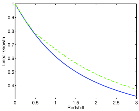
Figure 1: The solid line represents the linear growth of structure, normalised at redshift zero. The dotted line illustrates the influence of a $\delta$-function in $w$ at $z=0.5$ ($\epsilon=1$).

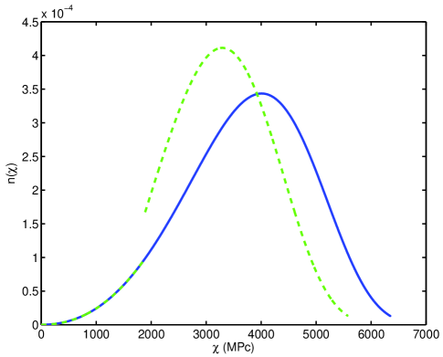
Figure 2: The number of galaxies as a function of coordinate distance, with (dashed) and without (solid) a delta function in $w(z)$ perturbing the standard $w=-1$ cosmology ($\epsilon=1$).

Conversely, the geometric factors described below suppress the shear signal. The coordinate distance $\chi(z)$ is now given by:

$$\chi(z,z^{\prime})=\frac{c}{H_{0}}\int_{0}^{z}\frac{\mathrm{d}z^{\prime\prime}}{\sqrt{\Omega_{m}(1+z^{\prime\prime})^{3}+\Omega_{\rm DE}f_{\rm DE}(z^{\prime},z^{\prime\prime})}}.$$ (14)

In the context of equation (2), the most significant change made by this modified distance-redshift relation is a shift in the galaxy probability distribution $n(\chi)$. A cosmic shear survey will typically use photometric redshift information to evaluate $n(z)$, whereas the shear signal itself is sensitive to $n(\chi)$, where $n(\chi)\mathrm{d}\chi=n(z)\mathrm{d}z$. Fig. 2 demonstrates how a $\delta$-function shifts $n(\chi)$ to be closer, for a given $n(z)$. Subsequently, the shear is reduced, since it accumulates over a shorter distance, and the lensing efficiency is lowered.

In summary, with a more positive w(z), the lensing signal is supported by the strengthened presence of structure, but reduced by the effects on the lens geometry.

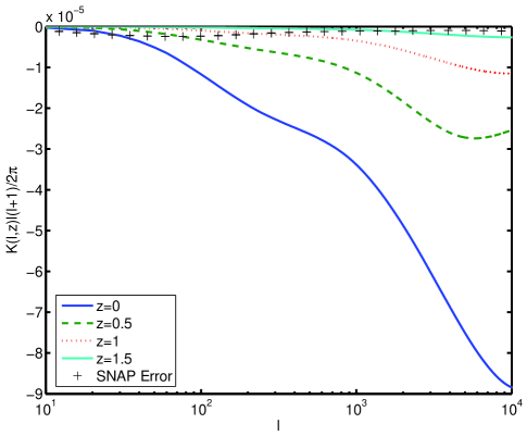
Figure 3: The kernel at z=0,0.5,1, and 1.5, along with the anticipated band-averaged errors for the SNAP wide survey. This illustrates the net decrement in the observed shear signal due to a positive perturbation in $w(z)$. By considering the nature of equation (12), one can begin to visualise the weight function taking shape.

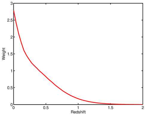
Figure 4: The weight function corresponding to the fiducial cosmic shear survey (SNAP wide) using a single redshift bin.

III Analysis of Results

In this section, our aim is to improve our understanding of how cosmic shear detects dark energy by utilising the weight function approach described in §IIC.

III.1 The Kernel

Selected redshift slices from $K(\ell,z)$, the functional derivative of the shear power spectrum, are shown in Fig. 3. Here we follow convention by multiplying the shear $C_{\ell}$ by a factor of $\ell(\ell+1)/2\pi$. Therefore, since we have amplified the higher multipoles, it is not surprising to see that this is where the greatest change occurs. The behaviour of these multipoles, which correspond to lensing by the non-linear regime of the matter power spectrum, will determine the form of the weight function due to their large signal-to-noise ratio.

The fact that the kernel is negative suggests that there has been a net decrease in the observed shear, and thus the modification of the comoving angular diameter distance has prevailed over the matter power spectrum, which is strengthened by the decreased growth rate.

III.2 The Weight Function

Let us now consider the nature of the weight function for the fiducial cosmic shear survey (SNAP) described in §II.1.2, as shown in Fig. 4.

The reason for the peak at redshift zero is twofold. Clearly, this is the point at which dark energy is most prevalent - the sensitivity of cosmic shear is primarily governed by the decay of $\Omega_{\rm DE}$ - but another contributing factor is that we have fixed our parameters at redshift zero, and so by introducing a perturbation in $w$ at a lower redshift, the cosmology will be modified across a wider redshift range. We therefore anticipate that using the data to constrain parameters such as $\Omega_{m}$, would strengthen the weight function at higher redshifts.

Another feature of this plot is the fairly abrupt change of gradient at around $z\sim 0.25$. To explain this we will first have to consider the separate contributions from structure and geometry.

We calculated a weight function which corresponds to the influence felt by cosmic shear via changes in the growth of structure. This was evaluated by only inserting the delta function into the equation of state experienced by the matter power spectrum. This approach was reapplied for the comoving angular diameter distance. In Fig. 5, the weight functions for these two effects are plotted.

The weighting functions corresponding to geometry and structure growth appear quite similar and are both relatively straightforward, with no sudden changes in gradient.

The structure growth weight function is slightly more strongly peaked at lower redshift and this is important in understanding the full cosmic shear weight function. We interpret this focus on lower redshift as being due to two factors. Firstly the lensing efficiency (Equation 3) peaks at a redshift intermediate between us and the background galaxies. Secondly due to growth of structure the conglomeration of matter is more prevalent at low redshift. This becomes particularly apparent when we recall that the matter power spectrum is proportional to the square of the growth factor.

Additionally, the nature of the nonlinear correction is such that the higher the power spectrum, the greater the factor of amplification. For example, at $k\sim 1Mpc$ and $z=0$, a 5% increase in linear growth can typically lead to a 15% increase in power. Therefore $w(z)$ imparts the greatest influence on low-redshift nonlinear structure.

Since the structure growth and geometric influences work in opposite directions on the cosmic shear power spectrum then the total weight function is expected to be roughly some difference between these two weighting functions. The line marked “Combined” in Fig. 5 is generated by subtracting the structural weight function from a version of the geometric one, scaled-up in accordance with its greater influence. This factor is given by the ratio of $\partial C_{\ell}/\partial w_{DA}$ to $\partial C_{\ell}/\partial w_{G}$. From §V this is found to be 1.84. Combinining weight functions in this manner is valid when the dominant multipoles (those with the highest signal-to-noise) exhibit the same response to the equation of state. We find this to be a remarkably accurate reproduction of the SNAP weight function, thereby verifying our earlier analysis.

Finally, we investigate the effects of modifying our constraints. Fig. 6 illustrates the response of the weight function to a reduction in the upper multipole limit ($\ell<1,000$), as would be necessary in the case of severe baryon contamination. Now we are no longer sensitive to the non-linear regime, and have thus become dominated by the geometric signal.

In order to assess the consequences of normalising the growth factor at high redshift, we utilise the CMB instead of $\sigma_{8}$ to fix the amplitude of the matter power spectrum. As illustrated by the dotted line in 6 the weight function is pushed to slightly higher redshifts. Note that this rise is attenuated by the loss of the aforementioned cancellation effect between stucture and geometry. By constraining the growth factor at high redshift, we have reversed the effect of the $\delta$ function observed in Fig. 1. Therefore a slower rate of structure growth will now reduce the prevalence of structure.

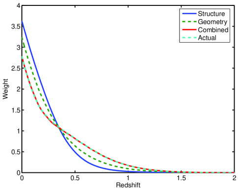
Figure 5: These weight functions arise when we consider modifying the geometric terms and structure growth independently. We then use a weighted combination of the two, as descibed in the text, to see how the form of the complete weight function emerges. The actual weight function is also provided to illustrate the accuracy of this approach.

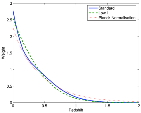
Figure 6: Here we experiment with alternative constraints. The solid line is the standard SNAP weight function from Figure 4. The dashed line represents the effect of enforcing a more conservative upper limit of $\ell<10^{3}$. The dotted line illustrates the effect of constraining the amplitude of the matter power spectrum at $z\sim 1000$ instead of $z=0$, as may be achieved with anticipated data from Planck

III.3 Accuracy

The weight function is only expected to be completely accurate when the true equation of state $w(z)$ is very close to the fiducial model. To test the accuracy of the weight function we compare the best fit value of $w$ (attained by minimisation of $\chi^{2}$) with that from integration over the weight function (11). The true parameterisation is taken to be of the form $w(z)=w_{0}+w_{a}(1-a)$, and we consider the range $-1.5<w_{0}<-0.5$ and $-1<w_{a}<1$.

The resulting errors displayed in Fig. 7 illustrate that the weight function approach is sufficiently accurate to apply to any shear survey currently under consideration. The perfect accuracy attained when $w_{a}=0$ should be regarded as an artefact of the calculation, since the form of the weight function becomes redundant. However it is notable that even within the extreme regions of the plot, much of which lies beyond current observational constraints, the weight function remains an excellent predictor of the fitted value.

If $w$ is strongly negative then we would expect the weight function to fall off more rapidly, in accordance with the decline of $\Omega_{\rm DE}$. While this effect can be seen in the plot, where the diagonal on which $w^{\rm fit}=-1$ provides higher accuracy, the deviation elsewhere is not of great significance.

Nonetheless, it may be worthwhile to reevaluate the weight function in future, using the observed $w^{\rm fit}$ as the fiducial model.

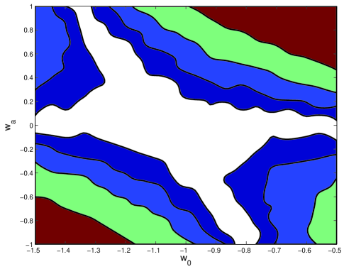
Figure 7: The contours above correspond to discrepancies of 0.002, 0.005, 0.01 and 0.02 between the the true value of $w^{\rm fit}$, and that attained by integration over the weight function.

IV Tomography

By dividing the pool of source galaxies into two redshift bins, we can produce shear power spectra from the two auto-correlations, and a cross-correlation. This provides us with invaluable information regarding the evolution of the shear signal, and can considerably improve constraints on various cosmological parameters. However, the gain from further subdivision of bins is limited due to their increasingly correlated shear signals Hu (1999).

To evaluate the cross-correlation, the necessary modification to equation (2) is achieved by replacing $g(\chi)^{2}$ with $g_{A}(\chi)g_{B}(\chi)$ where A and B are the two redshift bins, split at approximately $z=1.43$. Following Refregier Refregier et al. (2004), we produce our binned galaxy distributions, $n(\chi)$, by modifying the constants and applying a smear factor to equation (5). Fig. 8 compares the weight functions of the three power spectra.

In the high-z bin, we see further enhancement of the gradient change seen in Fig. 4, as the perturbed structure plays an increasingly important role.

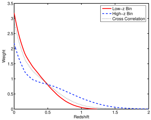
Figure 8: The weight functions for the two redshift bins, and their cross-correlation.

V Distance or Growth?

In §2 we noted how cosmic shear can reveal dark energy via two mechanisms. A change in our expansion history can alter both the distance-redshift relation, and structure growth. In terms of optics, this is analogous to a modification of lens geometry and focal length respectively.

Hereafter, we treat these influences separately, by introducing the effective equations of state $w_{G}$ and $w_{DA}$. These refer to the equations of state experienced by growth of structure and comoving angular diameter distance respectively. Can cosmic shear differentiate between these quantities?

We utilise the standard Fisher formalism to produce the contour plot for the SNAP-like shear survey shown in Fig. 9

$$F_{\alpha\beta}=\sum_{l}\frac{\displaystyle\partial C_{l}}{\displaystyle\partial p_{\alpha}}\frac{\displaystyle\partial C_{l}}{\displaystyle\partial p_{\beta}}/\sigma^{2}(l).$$ (15)

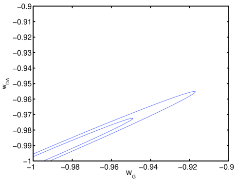
Figure 9: Contours on the dark energy parameter split into its contributions to the growth factor and the angular diameter distance (all other cosmological parameters are kept fixed). The degeneracy direction shows that the two effects partially cancel each other, and that the equation of state is slightly better constrained via the angular diameter distance.

While we can derive little from the size of the contours, since we have not marginalised over any other parameters, the correlated errors reinforce several points.

The error in $w_{G}$ is nearly twice that of $w_{DA}$, while the orientation of the ellipse is such that their values clearly have opposing effects on observations. This verifies the findings of § III.2 using an independent approach, and is in agreement with Abazajian & Dodelson Abazajian and Dodelson (2003).

VI Comparison of Lensing Surveys

We now vary the survey parameters in order to see how the weight function is affected. First, we consider a survey originating from the highest possible redshift, lensing of the Cosmic Microwave Background (CMB). At the other end of the spectrum, the CFHTLS will sample a relatively low redshift distribution of galaxies.

VI.1 The Cosmic Microwave Background

Lensing of the CMB can in principle be estimated from observations of higher order moments of the temperature maps, as well as from polarization observations (see e.g. Hu & Okamoto Hu and Okamoto (2002) for more information).

To evaluate the cosmic shear experienced by the CMB, we create an infinitesimal redshift bin at $z\sim 1100$. This simplifies the lensing efficiency to

$$g(\chi)=2\frac{\displaystyle\chi(\chi_{\rm rec}-\chi)}{\displaystyle\chi_{\rm rec}},$$ (16)

where $\chi_{\rm rec}$ is the distance to $z=1100$. Note that the relevant observable is now the deflection power spectrum, although this only differs from the standard convergence power spectrum by a factor of 4/$\ell(\ell+1)$. The anticipated errors of Planck are used, as shown in Figure 3 of Hu Hu (2002).

The resulting weight function is shown by the dotted line in Fig. 10. It is somewhat counter-intuitive to see that the CMB weight function is less sensitive than SNAP within the high-redshift regime. Once again, the answer lies in the combination of geometric and structural factors. Note that for the CMB, $\chi_{\rm rec}$ is so large that $w$ has a minimal impact on the lensing efficiency at low $\chi$, since $g(\chi)\simeq 2\chi$ and the distances cancel on substituting this into Equation 2. Thus, when we perturb $w$, the change in the growth of structure is the dominant factor, and so we lose the partial cancellation effect which had pushed the SNAP weight function to higher redshifts.

VI.2 Ground-Based Lensing

Here we assess two future projects, whose anticipated survey parameters are outlined below.

For the CFHTLS, the number denisty of galaxies is reduced to $n_{g}=26$ ${\rm arcmin}^{-2}$. The galaxy redshift distribution, $n(z)$, is taken from the VIRMOS estimation by van Waerbeke et al. Van Waerbeke et al. (2002). In the context of equation 5 we now have $\alpha=2$, $\beta=1.2$, and $z_{0}=0.44$. The rms shear $\sigma_{\gamma}=0.31$, and the area of the survey is 170 square degrees. The resulting weight function is shown by the dashed line in Fig. 10. The sensitivity at high redshift is limited by the depth of the survey.

For the LSST, the number denisty of galaxies $n_{g}=65$ ${\rm arcmin}^{-2}$, and the rms shear $\sigma_{\gamma}=0.16$ . The redshift distribution is adopted from Song & Knox Song and Knox (2004). The resulting weight function is the dot-dash line in Fig. 10. The close resemblance to the SNAP plot is not surprising given their similar redshift distributions. And while the survey is much wider (30,000 square degrees), it should be noted that the weight function is in fact independent of the sky coverage, since this just enters as a constant multiple of the errors.

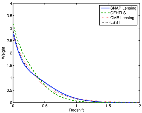
Figure 10: A comparison of lensing surveys. Despite the wide variety of parameters, as outlined in the text below, the differences in the weight functions are minor. The dot-dash line corresponding to the LSST is barely distinguishable from the SNAP one.

VII Comparing Alternate Probes of Dark Energy

We turn our attention to Fig. 11 which shows the response of different methods to the equation of state.

VII.1 Benchmark

The ‘benchmark’ is the weight attributed to a purely hypothetical survey which equally examines dark energy within all redshift bins. That is to say, it represents a neutral (albeit somewhat unphysical) observation whereby the value of $w$ for each quanta of dark energy is measured.

In the context of equation (12), we have no redshift dependency so $K(l,z)={\rm const.}$, and $\sigma^{2}(z)\propto(1+z)^{3}$ due to the amount of dark energy present.

This leads us to a weight function which is a (normalised) plot of volume versus redshift.

$$\Phi_{bench}(z)=\frac{\displaystyle 2}{\displaystyle(1+z)^{3}}$$ (17)

This is taken as a reference point, from which we can identify the redshift bias of more complex methods. We see that a cosmic shear survey with the SNAP parameters comes quite close to this benchmark.

VII.2 Type 1A Supernovae

The dashed line in Fig. 11 is calculated for the proposed SNAP supernovae study, where supernovae are assumed to be uniformly distributed between redshifts 0.1 and 1.7, and errors are taken to be inversely proportional to the coordinate distance.

One might intuitively expect supernovae to probe higher redshift regions than cosmic shear, since lensing mostly occurs approximately mid-way between source and observer. However, Section IID has already outlined why the combination of structural and geometric factors have pushed the sensitivity to higher $z$. Moreover, the poor accuracy of high-$z$ supernovae has the opposite effect. The resulting weight function is shown in Fig. 11 and was also calculated in Saini et al Deep Saini et al. (2003). It should be noted that even a high-redshift supernovae survey actually measures $w(z)$ at a redshift lower than a shallow cosmic shear survey.

Let us now consider a possible consequence of surveys which have significantly different weight functions. Disparity in the constant-$w$ fits may not necessarily indicate inconsistent data. For instance, if we adopt a varying equation of state of the form $w=w_{0}+w_{a}(1-a)$ then in order for $w^{fit}_{Shear}$ to differ from $w^{fit}_{SNAe}$ by 5% we would require $|w_{a}|>0.7|w_{0}|$.

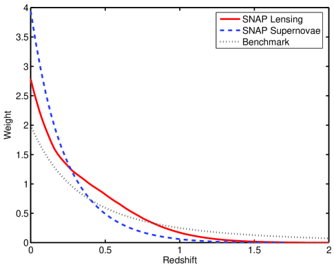
Figure 11: The weight functions for lensing of the cosmic shear (solid), supernovae evenly distributed from $z=0.1$ to $z=1.7$ (dashed), and benchmark (dotted). Cosmic shear probes the equation of state at higher redshifts than the supernovae (for SNAP-like surveys), as explained in the text.

VIII Discussion

We have revealed the manner in which cosmic shear probes the dark energy equation of state. The survey specifications of SNAP, due for launch in 2014, have been taken as an example. However, it should be noted that in general, weight functions are invariant to the absolute errors of the observation, and as such the survey-dependency of the weight function is small.

The important point is that interpreting the equation of state via weight functions circumvents the problem of which parameters to use for the evolution of the dark energy. A parameterization can be decided on, but if the true equation of state does not have the functional form assumed, the meaning of the coefficients can still be interpreted clearly in terms of the true variation of the equation of state.

The weight function for cosmic shear, which describes the redshifts to which we are sensitive, is found to differ significantly from that of a supernovae survey. Therefore a discrepancy in the values of $w$ may be indicative of an evolving equation of state.

Remarkably, the competing factors of structure and geometry ensure that cosmic shear will be more sensitive to the high-redshift values of $w(z)$ than lensing of the CMB. Since the primary goal is to detect a deviation from $w=-1$, and many theories suggest that this would be most prominent at high redshift, then these high-z sensitivities are particularly desirable.

The way in which $w$ modifies the nonlinear correction to the matter power spectrum remains an issue, and we await the outcome of large N-body simulations of quintessence cosmologies in order to progress further.

The principal component analysis of Huterer Huterer and Starkman (2003) also investigates the sensitivity of supernova data to the equation of state as a function of redshift, focussing on finding the modes that can be well constrained by the data. The extension of this work to compare supernova and weak lensing data by Knox et al. Knox et al. (2004) supports our findings.

This work is complementary to that of Hu (2004) Hu (2004) which analyses the change of various measures (e.g. angular diameter distance as a function of redshift) on changing w from a cosmological constant to an alternative model, at the same time modifying the amount of dark energy $\Omega_{\rm DE}$ to keep the angular diameter distance to the CMB constant. We have fixed the cosmological parameters at redshift zero for the current analysis and an investigation into the multitude of alternative priors is beyond the scope of this work. Our approach differs from the investigation of Hu in that it is not dependent on specific modifications to the dark energy equation of state, and investigates cosmic shear specifically.

There are a number of routes down which this work could progress. Specifically, the fitting of extra parameters such as $w_{0}$ and $w_{1}$ (for $w(z)=w_{0}+w_{1}z$) which has been done for the supernova weight function in Deep Saini et al. (2003) or a reconstruction of $w(z)$ in redshift bins. This could even be extended to other cosmological parameters such as $\Omega_{m}$. Maor et al. Maor et al. (2002) have highlighted the problems associated with determining $w$ when $\Omega_{m}$ is not tightly constrained. In addition, it would be instructive to compare the standard cosmic shear weight function with that of the Jain & Taylor Jain and Taylor (2003) approach.

The illustrative nature of weight functions provides an intuitive insight into the meaning of experimental results. Furthermore, we believe this approach will prove useful in optimising future surveillance strategies. For instance, it may become desirable to probe a particular redshift regime of $w(z)$, at which point the weight functions of various surveys should be considered. This is most readily achieved by careful selection of the source distribution n(z). However, in doing so we must ensure the overall accuracy of the measurement is not compromised.