Challenges for Inflationary Cosmology

Abstract

Inflationary cosmology has provided a predictive and phenomenologically very successful scenario for early universe cosmology. Attempts to implement inflation using scalar fields, however, lead to models with serious conceptual problems. I will discuss some of the problems, explain why string theory could provide solutions to a subset of these problems, and give a brief overview of “string gas cosmology”, one of the approaches to merge string theory and early universe cosmology.

1 Introduction

As is well known, inflationary cosmology was developed in order to resolve some conceptual problems of standard big bang cosmology such as the horizon and flatness problems [1]. The most important success of inflation, however, is that it provides a causal mechanism for generating cosmological fluctuations on microscopic scales which evolve into the perturbations which are observed in the large-scale structure of the universe and the anisotropies in cosmic microwave background (CMB) temperature maps [2] (see also [3]). In the simplest models of inflation, models in which inflation is driven by a single scalar field, the predicted spectrum of fluctuations is adiabatic and almost scale-invariant. These predictions have been confirmed with unprecedented accuracy by recent observations, in particular by the WMAP maps of the temperature of the CMB [4].

Before claiming that early universe cosmology is solved, we should recall the status of the previous paradigm of early universe cosmology, the “standard big bang” model. It explained the relation between redshift and distance of galaxies. Without doubt, however, its biggest success was that it predicted the existence and black body nature of the cosmic microwave background. This spectacular quantitative success, however, did not imply that the theory was complete. In fact, one of the gravest conceptual problems of “standard big bang” cosmology is related to its greatest successes: the theory does not explain why the temperature of the black body radiation is nearly isotropic across the sky.

In the following I will argue that the calculations involved in the derivation of the spectrum of cosmological fluctuations contain in themselves the seeds for their incompleteness. Other conceptual problems of standard big bang cosmology were not resolved by inflation and thus re-appear in the list of conceptual problems of inflationary cosmology.

Most models of inflation are formulated in the context of Einstein gravity coupled to a matter sector which contains the “inflaton”, a new scalar field. Some (but not all) of the problems discussed below are specific to such scalar field-driven models of inflation. I will focus on this class of inflationary models.

2 Conceptual Problems of Scalar Field Driven Inflation

2.1 Fluctuation Problem

As was mentioned in the Introduction, inflationary cosmology produces an almost scale-invariant spectrum of cosmological fluctuations [2]. A concrete model of scalar field-driven inflation also predicts the amplitude of the spectrum. The problem is that without introducing a hierarchy of scales into the particle physics model, the predicted amplitude of fluctuations exceeds the observational results by several orders of magnitude. For example, if the potential of the inflaton (the scalar field driving inflation) $\varphi$ has the form

$$V(\varphi)\,=\,{1\over 4}\lambda\varphi^{4}\,,$$ (1)

then a value of

$$\lambda\,\sim\,10^{-12}$$ (2)

is required in order that the predicted amplitude of the spectrum matches with observations. It has been shown [5] that this problem is quite generic to scalar field-driven inflationary models (counterexamples, however, can be constructed - I thank David Lyth for pointing this out to me). Given that one of the main goals of cosmological inflation is to avoid fine tunings of parameters of the cosmology, it is not very satisfying that fine tunings re-appear in the particle physics sector.

2.2 Trans-Planckian Problem

The most important success of inflationary cosmology is that scales of cosmological interest today start out with a wavelength smaller than the Hubble radius at the beginning of the period of inflation. This allows the development of a causal theory of the generation and evolution of fluctuations (see e.g. [6] for a comprehensive review, and [7] for a shorter summary). In most scalar field-driven inflationary models, in particular those of chaotic [8] type, the period of inflation lasts much longer than the minimal number of e-foldings required for successful resolution of the horizon and flatness problems. In this case, the physical wavelength of comoving modes which correspond to today’s large-scale structure was smaller than the Planck length at the time $t_{i}$ when the period of inflation began (see Fig. 1 (taken from [10]) for a sketch of the space-time geometry).

It is clear that both key ingredients of scalar field-driven inflationary cosmology, namely the description of space-time by General Relativity, and the use of semi-classical scalar fields to model matter, break down on scales smaller than the Planck length. However, the spectrum of cosmological fluctuations is determined by solving the equations for perturbations as an initial value problem, starting off all modes at time $t_{i}$ in their vacuum state. The unknown physics which describes space-time and matter on Planck scales must enter into the calculation of the spectrum of cosmological fluctuations. The key question [9] is whether the conclusions derived from the usual computations are sensitive to the new physics.

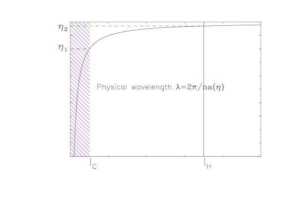
Figure 1: Space-time sketch showing how the physical wavelength (horizontal axis) of a fluctuation with fixed comoving frequency $n$ increases in time (vertical axis) during the period of inflation. The variable $\eta$ denotes conformal time, the length $l_{c}$ is the Planck length (or whatever the critical ultraviolet length of the new physics is), $l_{H}$ denotes the Hubble radius.

Let us give an argument why large deviations in the predictions could be expected [10]. Returning to Fig. 1, we see that the evolution of the perturbations for any mode can be divided into three phases. In the first phase ($\eta<\eta_{1}$), the wavelength is smaller than the Planck length and the evolution is crucially influenced by the new physics. In Period 2 ($\eta_{1}<\eta<\eta_{2}$), the wavelength is larger than the Planck length but smaller than the Hubble length. In this period, the fluctuations will perform quantum vacuum oscillations, as described by the usual theory of cosmological fluctuations [6, 7]. Finally, in the third period (wavelength larger than the Hubble scale), the fluctuations freeze out, are squeezed, and become classical. Assume now that the evolution in Phase 1 is such that it is non-adiabatic from the point of view of the usual equations. In this case, an initial state at $t_{i}$ minimizing the energy (in the frame given by the cosmological background) will evolve into an excited state at the time $t_{c}(k)$ when the mode $k$ enters Period 2. Since different modes spend a different amount of time in Period 1, one should expect that the excitation level at time $t_{c}(k)$ will depend on $k$ (in fact, a blue spectrum will be produced), in contrast to what happens in the usual analysis (which yields a scale-invariant spectrum). A toy model of new physics which gives this result was presented [10]. It is based on describing the evolution of fluctuations by means of a modified dispersion relation $\omega_{p}(k_{p})$, where the subscripts $p$ indicate physical (rather than comoving) values.

Obviously, more conservative choices for describing the evolution of fluctuations in the presence of new physics, e.g. the “minimal trans-Planckian” prescription of starting the perturbation modes off in a vacuum state at the time that the wavelength equals the scale of new physics [11, 12] yield corrections to the usual predictions which are small (see e.g. [13] for a review with references to original works). It was suggested [14, 15] that back-reaction effects of ultraviolet modes might lead to stringent limits on the amplitude of possible trans-Planckian effects. However, it was recently shown [16] that the back-reaction of ultraviolet modes in fact mainly leads to a renormalization of the cosmological constant, and that the constraints on the magnitude of possible trans-Planckian effects which are consistent with having a period of inflation are thus greatly relaxed.

The “trans-Planckian” problem for inflationary cosmology should in fact not be viewed as a problem at all. Rather, it opens an exciting window to probe Planck-scale physics using current cosmological observations.

2.3 Singularity Problem

The famous Hawking-Penrose theorems [17] prove that standard big bang cosmology is incomplete since there is an initial singularity. These theorems assume that matter has an equation of state with non-negative pressure, and that space-time is described by the Einstein equations. As was shown recently [18], these theorems can be generalized to apply to scalar field-driven inflationary cosmology. It is shown that there are some geodesics which cannot be extended arbitrarily far into the past. An intuitive way to understand this result is the following. We focus on some time $t$ during the phase of inflation. Some fluctuations will be present at this time. Evolving these fluctuations back in time, we find that they will come to dominate the energy density at some time in the past. Prior to this time, the equation of state of scalar field matter thus has non-negative pressure, and the usual theorems apply. It thus follows that scalar field-driven inflationary cosmology is incomplete in the same way that standard big bang cosmology was incomplete.

2.4 Cosmological Constant Problem

The Achilles heel of scalar field-driven inflationary cosmology is the fact that the scenario uses the time-independent part of the potential energy of the scalar field to generate inflation. However, it is known that another form of constant potential energy, namely the quantum vacuum energy, does not gravitate. There is some unknown mechanism (the solution to the famous cosmological constant problem) which will explain why the quantum vacuum energy does not gravitate. The key challenge is to show why this mechanism does not also render the constant part of the scalar field potential energy gravitationally inert.

If the cosmological constant problem is solved by gravitational back-reaction (see [19] for a review of this scenario), then scalar field-driven inflation would be robust. However, this scenario [19] is at the moment rather controversial and requires much more development.

2.5 Who is the Inflaton?

The initial hope [1] was that the inflaton could be identified with the Higgs field of particle physics. However, because of hierarchy problems like (2), this hope was not realized. At the present time, although there are many possible models of inflation, there are no convincing theories based on well-established particle physics. Thus, an outstanding challenge for inflationary cosmology is to determine what the origin of the inflaton field is.

2.6 Why String Theory May Help

All of the above conceptual problems of current inflationary cosmology stem from our incomplete understanding of the fundamental physics at ultra-high energies. String theory is a candidate for a unified quantum theory of space-time and matter. Thus, it is challenging to study whether string theory provides a framework to possibly resolve the abovementioned problems.

Since string theory contains many scalar fields which are massless before supersymmetry breaking, it provides both candidates for the inflaton and an obvious way of producing the hierarchy of scales required to resolve the fluctuation problem. In the case of low-scale supersymmetry breaking, both the slow-rolling conditions and the size of the mass hierarchy might be sufficient for a successful inflationary model (I again thank David Lyth for stressing to be the caveat of low-scale supersymmetry breaking). Since string theory should describe the physics on all length scales, string theory should provide the correct equation to describe cosmological fluctuations throughout the evolution of the universe, thus resolving the trans-Planckian problem. Finally, it is hoped that string theory will resolve cosmological singularities (and a concrete framework in which this happens exists [20]). The only of the conceptual problems of inflation which at the present time does not appear to be solvable within the current knowledge of string theory is the cosmological constant problem.

3 Challenges for String Cosmology

However, when considering string theory as a framework for early universe cosmology, an immediate obstacle appears: at a perturbative level, critical superstring theory is consistent only in nine spatial dimensions. Why do we only see three spatial dimensions? There is evidence that the non-perturbative formulation of string theory (“M-theory”) in a different limit leads to 11-d supergravity. Once again, the predicted number of spatial dimensions is not what is observed.

The traditional approach to resolving this problem is to assume that six (or seven) of the spatial dimensions are compactified on a string-scale manifold and hence are invisible to us. From the point of view of cosmology there are two immediate questions: First, what selects the number of dimensions which are compactified, and second, why is the radius of compactification stable? In a more modern approach (“brane world scenarios”), the matter fields of the particle physics standard model are taken to be confined to a 3-brane (three spatial dimensions) which lives in the higher-dimensional bulk. Again, however, the question as to why a 3-brane (and not a brane of different dimensionality) is the locus of our matter fields arises (there has been an interesting work on this issue [21]).

Thus, before addressing the issue of whether string theory can provide a convincing realization of cosmological inflation, string cosmology should explain why there are only three large spatial dimensions. The next section will briefly review a string-based scenario of the early universe which may provide an explanation. Once three spatial dimensions have been selected as the only ones to become large, string theory offers various mechanisms of obtaining inflation [22, 23].

4 Overview of String Gas Cosmology

A frequent criticism of current approaches to string cosmology is that string theory is not developed enough to consider applications to cosmology. In particular, one may argue that string cosmology must be based on a complete non-perturbative formulation of string theory. By focusing on the effects of a new symmetry of string theory, namely t-duality, and of truly stringy degrees of freedom, namely string winding modes, the “string gas cosmology” program initiated in [20] (see also [24]) and resurrected [25] after the D-brane “revolution” in string theory hopes to make predictions which will also be features of cosmology arising from a non-perturbative string theory.

In string gas cosmology it is assumed that, at some initial time, the universe begins small and hot. For simplicity, we take space to be a torus $T^{9}$, with all radii $R$ equal and of string length. The t-duality symmetry - which is central to the scenario - is the invariance of the spectrum of free string states under the transformation

$$R\,\rightarrow\,1/R$$ (3)

(in string units). String states consist of center of mass momentum modes whose energy values are quantized in units of $1/R$, winding modes whose energy values are quantized in units of $R$, and oscillatory modes whose energy is independent of $R$. If $n$ and $m$ denote the winding and momentum numbers, respectively, then the spectrum of string states is invariant under (refdual1) if

$$(n,m)\,\rightarrow\,(m,n)\,.$$ (4)

T-duality is also a symmetry of non-perturbative string theory [26].

The action of the theory is given by the action of a dilaton-gravity background (a background for which the action has t-duality symmetry in contrast to what would be the case were we to fix the dilaton and consider the Einstein action only) coupled to a matter action describing an ideal gas of all string matter modes. In analogy to standard big bang cosmology we assume that at the initial time all matter modes (in particular string momentum and winding modes) are excited. We call these initial conditions “democratic” - since all radii are taken to be equal - and “conservative” - since hot rather than cold initial conditions are assumed. If we start from the Type II superstring corner of the M-theory moduli space, there will be branes of various dimensionalities in addition to the fundamental strings.

Using the dilaton gravity equations of motion is can be shown [27, 28] that negative pressure leads to a confining potential for the radius of the tori. Thus, the presence of string winding modes will prevent the spatial dimensions from expanding. String momentum modes will not allow space to contract to zero size. There will be a preferred radius (the “self-dual” radius which in string units is $R=1$). Spatial dimensions can only become large if the string winding modes can annihilate (we assume zero net winding number). This cannot occur in more than three large dimensions because the probability for string world sheets to intersect will be too small. In three dimensions, as studied in detail elsewhere [29], the winding modes will fall out of equilibrium as $R$ increases, and they can annihilate sufficiently fast to allow these three dimensions to expand without bounds. Thus, in the Type II corners of the M-theory moduli space, string gas cosmology provides a possible solution of the dimensionality problem facing any string cosmology. By t-duality, a universe with $R<1$ is equivalent to a universe with $R^{\prime}=1/R>1$. Hence [20], string gas cosmology also provides a nonsingular cosmological scenario.

Note that the existence of fundamental strings or stable 1-branes is crucial to having $D=3$ emerge dynamically as the number of large spatial dimensions. In the 11-d supergravity corner of the M-theory moduli space it in unlikely [30] that $D=3$ will emerge as the number of large spatial dimensions. There are, however, possible loopholes [31] in this conclusion based on the special role which intersections of D=2 and D=5 branes can play.

Once three spatial dimensions start to expand, the radius of the other dimensions (the “radion”) will automatically be stabilized at the self-dual radius [32]. This conclusion is true for a background given by dilaton gravity. To make contact with the late-time universe, a mechanism to stabilize the dilaton must be invoked. It has been shown [33] that, at least in the case of one extra spatial dimension, the radion continues to be stabilized after the dilaton is fixed. Crucial to reach the conclusion [33, 34, 35] is the inclusion in the spectrum of string states of states which become massless at the self-dual radius.

Thus, string gas cosmology appears to provide a scenario which provides a nonsingular cosmology, explains why D=3 is the number of large spatial dimensions at late times, and incorporates radion stabilization without any extra physics input. The two main challenges to the scenario are to provide a mechanism for dilaton stabilization and to provide a solution to the flatness problem. It would be nice if string gas cosmology would provide a natural mechanism for inflating the three large dimensions. There are some initial ideas [36] towards this goal.

References

- [1] A. H. Guth, Phys. Rev. D 23, 347 (1981).
- [2] V. F. Mukhanov and G. V. Chibisov, JETP Lett. 33, 532 (1981) [Pisma Zh. Eksp. Teor. Fiz. 33, 549 (1981)]; G. V. Chibisov and V. F. Mukhanov, Mon. Not. Roy. Astron. Soc. 200, 535 (1982).
- [3] V. N. Lukash, Sov. Phys. JETP 52, 807 (1980) [Zh. Eksp. Teor. Fiz. 79, 1901 (1980)]; W. H. Press, Phys. Scr. 21, 702 (1980); K. Sato, Mon. Not. Roy. Astron. Soc. 195, 467 (1981).
- [4] C. L. Bennett et al., Astrophys. J. Suppl. 148, 1 (2003) [arXiv:astro-ph/0302207].
- [5] F. C. Adams, K. Freese and A. H. Guth, Phys. Rev. D 43, 965 (1991).
- [6] V. F. Mukhanov, H. A. Feldman and R. H. Brandenberger, Phys. Rept. 215, 203 (1992).
- [7] R. H. Brandenberger, Lect. Notes Phys. 646, 127 (2004) [arXiv:hep-th/0306071].
- [8] A. D. Linde, Phys. Lett. B 129, 177 (1983).
- [9] R. H. Brandenberger, arXiv:hep-ph/9910410.
- [10] J. Martin and R. H. Brandenberger, Phys. Rev. D 63, 123501 (2001) [arXiv:hep-th/0005209]; R. H. Brandenberger and J. Martin, Mod. Phys. Lett. A 16, 999 (2001) [arXiv:astro-ph/0005432].
- [11] U. H. Danielsson, Phys. Rev. D 66, 023511 (2002) [arXiv:hep-th/0203198].
- [12] V. Bozza, M. Giovannini and G. Veneziano, JCAP 0305, 001 (2003) [arXiv:hep-th/0302184].
- [13] J. Martin and R. Brandenberger, Phys. Rev. D 68, 063513 (2003) [arXiv:hep-th/0305161].
- [14] T. Tanaka, arXiv:astro-ph/0012431.
- [15] A. A. Starobinsky, Pisma Zh. Eksp. Teor. Fiz. 73, 415 (2001) [JETP Lett. 73, 371 (2001)] [arXiv:astro-ph/0104043].
- [16] R. H. Brandenberger and J. Martin, arXiv:hep-th/0410223.
- [17] S.W. Hawking and G.F.R. Ellis, “The Large Scale Structure of Space-Time” (Cambridge Univ. Press, Cambridge, 1973).
- [18] A. Borde and A. Vilenkin, Phys. Rev. Lett. 72, 3305 (1994) [arXiv:gr-qc/9312022].
- [19] R. H. Brandenberger, arXiv:hep-th/0210165.
- [20] R. H. Brandenberger and C. Vafa, Nucl. Phys. B 316, 391 (1989).
- [21] M. Majumdar and A. Christine-Davis, JHEP 0203, 056 (2002) [arXiv:hep-th/0202148].
- [22] G. R. Dvali and S. H. H. Tye, Phys. Lett. B 450, 72 (1999) [arXiv:hep-ph/9812483]; S. H. S. Alexander, Phys. Rev. D 65, 023507 (2002) [arXiv:hep-th/0105032]; C. P. Burgess, M. Majumdar, D. Nolte, F. Quevedo, G. Rajesh and R. J. Zhang, JHEP 0107, 047 (2001) [arXiv:hep-th/0105204].
- [23] S. Kachru, R. Kallosh, A. Linde, J. Maldacena, L. McAllister and S. P. Trivedi, JCAP 0310, 013 (2003) [arXiv:hep-th/0308055].
- [24] J. Kripfganz and H. Perlt, Class. Quant. Grav. 5, 453 (1988).
- [25] S. Alexander, R. H. Brandenberger and D. Easson, Phys. Rev. D 62, 103509 (2000) [arXiv:hep-th/0005212].
- [26] J. Polchinski, “String Theory, Vols. 1 & 2” (Cambridge Univ. Press, Cambridge, 1998).
- [27] A. A. Tseytlin and C. Vafa, Nucl. Phys. B 372, 443 (1992) [arXiv:hep-th/9109048].
- [28] G. Veneziano, Phys. Lett. B 265, 287 (1991).
- [29] R. Brandenberger, D. A. Easson and D. Kimberly, Nucl. Phys. B 623, 421 (2002) [arXiv:hep-th/0109165].
- [30] R. Easther, B. R. Greene, M. G. Jackson and D. Kabat, Phys. Rev. D 67, 123501 (2003) [arXiv:hep-th/0211124].
- [31] S. H. S. Alexander, JHEP 0310, 013 (2003) [arXiv:hep-th/0212151].
- [32] S. Watson and R. Brandenberger, JCAP 0311, 008 (2003) [arXiv:hep-th/0307044].
- [33] S. P. Patil and R. Brandenberger, arXiv:hep-th/0401037.
- [34] T. Battefeld and S. Watson, JCAP 0406, 001 (2004) [arXiv:hep-th/0403075].
- [35] S. Watson, arXiv:hep-th/0404177.
- [36] R. Brandenberger, D. A. Easson and A. Mazumdar, Phys. Rev. D 69, 083502 (2004) [arXiv:hep-th/0307043].