Deflections of cosmic rays in a random component of the Galactic magnetic field

Abstract

We express the mean square deflections of the ultra-high energy cosmic rays (UHECR) caused by the random component of the Galactic magnetic field (GMF) in terms of the GMF power spectrum. We use recent measurements of the GMF spectra in several sky patches to estimate the deflections quantitatively. We find that deflections due to the random field constitute $0.03-0.3$ of the deflections which are due to the regular component and depend on the direction on the sky. They are small enough not to preclude the identification of UHECR sources, but large enough to be detected in the new generation of UHECR experiments.

I Introduction

The Galactic magnetic field (GMF) plays an important role in the propagation of cosmic rays even at highest energies. Expected deflections — of order few degrees or larger — are comparable or exceed the angular resolution of the existing cosmic ray experiments. Such deflections may therefore be observable. Their understanding is crucial when searching for sources of the highest-energy cosmic rays if the latter are charged particles.

The detailed study of deflections of ultra-high energy proton primaries in the GMF is particularly important if the deflections in extra-galactic magnetic fields are small. According to the results of Refs. Dolag this is likely to be the case (see, however, Ref. Sigl ).

The Galactic magnetic field has been shown to have both regular and turbulent components. The regular component is thought to have a spiral structure reminiscent of the Galactic arms with one or more reversals toward inner (and probably also outer) Galaxy and the magnitude of order $3~{}\mu$G in the vicinity of the Earth GMFmodels . The corresponding global model of GMF was constructed in Ref. Stanev:1996qj and is often used in the discussion of propagation of cosmic ray primaries in the Galaxy. According to this model, protons with energy $4\times 10^{19}$ eV can be deflected in the regular GMF by $\sim 5^{\circ}$. There are indications that such a coherent deflections may indeed be present Tinyakov:2001ir ; Gorbunov:2002hk ; Teshima ; Tinyakov:2003nu in the cosmic ray data.

The random component of GMF causes the spread of arrival directions of UHECR around the mean position, thus diluting (and potentially destroying) important information about the actual location of the source Kronberg:1993vk . Under certain conditions on the magnetic field it may also lead to the “lensing” of cosmic rays Harari:2002dy ; Harari:2002fj provided the number of sources contributing to the observed UHECR flux is small, as is favored by the statistics of clustering Dubovsky:2000gv . Thus, the influence of a random fields is not simply destructive, but may give useful information on the cosmic rays and GMF itself.

Observationally, the magnitude of the random component of GMF is comparable to the magnitude of the regular one. However, the deflections of cosmic ray primaries in the random field are expected to be considerably smaller. Indeed, if the correlation length $L_{c}$ of the random component is much smaller than the propagation distance $D$, the deflections caused by the random field are proportional to $\sqrt{DL_{c}}$, see e.g. Ref. Berezinsky_book , while the deflections in the regular field are proportional to the distance $D$ itself. Usually the deflections in the random field are estimated as (see e.g. Ref. Roulet:2003rr )

$$\delta_{r}=0.6^{\circ}\cdot\left({10^{20}~{}{\rm eV}\over E/Z}\right)\left({B_{r}\over 4~{}\mu{\rm G}}\right)\sqrt{D\over 3~{}{\rm kpc}}\,\sqrt{L_{c}\over 50~{}{\rm pc}}\;,$$ (1)

where $E$ is the energy of CR primary and $B_{r}$ is the rms value of the random magnetic field strength. However, the global picture of GMF is very complicated. The magnetic field may be structured on relatively large scales, including possibility of magnetic bubbles, sheets, filaments, magnetic “winds” etc., so one cannot rely on (and be restricted to) a generic estimate uniformly over the whole sky.

The rms deflections of cosmic ray primaries in the random field are determined unambiguously by the magnetic field power spectrum. The latter can be extracted from observations, see e.g. Ref. Minter . Several existing measurements of the GMF power spectrum indicate that the correlation length can be large in some directions on the sky. In this case the deflections are no longer proportional to $\sqrt{DL_{c}}$, and the estimate (1) does not apply.

The purpose of the present paper is to estimate the deflections of UHECR primaries in the turbulent component of the Galactic magnetic field taking into account possible dependence of GMF parameters on the region of the sky and the possibility of large corelation length. We express the UHECR deflections directly through the observable parameters characterizing the power spectrum of the magnetic field. To this end we derive the relation between the mean square deflection and the power spectrum (PWS) of the GMF fluctuations. The result is most conveniently represented through the factor $R$ defined as

$$\frac{\delta_{r}}{\delta_{u}}=\frac{B_{r}}{B_{u,\bot}}\,R\;,$$ (2)

where $\delta_{r}$ and $\delta_{u}$ are deflections in the random and uniform components of GMF, respectively, and $B_{u,\bot}$ is a projection of a uniform field onto the direction orthogonal to the line of sight. The factor $R$ varies between 0 and 1 and is expressed in terms of the power spectrum of the random field by Eq. (28). Moreover, we show that it is a function of a single observable parameter $\theta_{c}$, the angular scale of the break in the relevant structure function of GMF. In the case of small correlation length when the estimate (1) applies, one has $R\sim\sqrt{\theta_{c}}$. The values of $R$ in our Galaxy derived from the existing observational data vary in the range $R\sim 0.03-0.3$. This implies typical deflections of a $4\times 10^{19}$ eV proton in the random field of order $0.2^{\circ}-1.5^{\circ}$ depending on the direction.

The paper is organized as follows. In Sect. II.1 we recall the relations between the power spectrum and the correlation length and introduce the notations. In Sec. III we describe existing observations of the random magnetic field, in particular, the random-to-uniform ratio and the parameters of the power spectrum. In Sect. IV we turn to the deflections of UHECR in the random magnetic field and derive the expression for the coefficient $R$. Sect. V summarizes our results.

II Turbulent field

II.1 Correlation length and power spectrum of GMF

To introduce notations and specify our assumptions, let us first consider the statistical properties of a random magnetic field $B_{a}({\bf r})$, where $a=1,2,3$. We define the Fourier components of the magnetic field according to

$$B_{a}({\bf r})=\int d^{3}qB_{a}({\bf q}){\rm e}^{i{\bf rq}}.$$

Here $B_{a}$ refers to the fluctuating component of the total magnetic field; the regular part of GMF has to be treated separately. In what follows we assume that the fluctuations obey Gaussian statistics and are spatially homogeneous and isotropic.

The last two assumptions deserve a comment. The statistical characteristics of the magnetic field are different in different sky patches. Our analysis and results should be applied to each of these patches separately. We assume that statistical properties of GMF are (approximately) constant over a single patch. Also, within one patch the magnetic field fluctuations may not be isotropic, with the preferred direction being set by the regular component of GMF. The present data are not sufficient to establish or rule out the isotropy of GMF fluctuations. With the more precise data this assumption may need to be reconsidered, and the analysis may need to be refined.

With the above assumptions, all correlators of the magnetic field can be expressed in terms of the two-point correlation function which can be written as

$$\langle B_{a}^{~{}}({\bf q})B_{b}^{*}({\bf q}^{\prime})\rangle={{\cal B}(q)\over 2q^{3}}(\delta_{ab}-n_{a}n_{b})\delta^{3}({\bf q-q^{\prime}}),$$ (3)

where $n_{a}=q_{a}/q$ is a unit vector in the direction of ${\bf q}$ and the projection tensor ensures the divergence-free nature of the magnetic field, $q_{a}B^{a}({\bf q})=0$. The dimensional normalization factors are chosen in such a way that the power spectrum ${\cal B}(q)$ has physical units of $B^{2}$, i.e. in our case it is measured in the units of (Gauss)². The correlation function of the magnetic field fluctuations is defined as

$$\xi(r) = \langle B_{a}({\bf r_{0}})B^{a}({\bf r_{0}+r})\rangle=\int\frac{d^{3}q}{q^{3}}\;{\cal B}(q)\;\mbox{e}^{-i{\bf qr}}{}$$ (4)

$$= 4\pi\int_{0}^{\infty}\frac{dq\,}{q}{\cal B}(q)\;\frac{\sin(qr)}{qr}~{}.{}{}{}{}{}{}{}{}{}{}{}{}{}{}{}{}{}{}{}{}{}$$

It determines the rms value of the field amplitude $B_{r}$,

$$B_{r}^{2}\equiv\langle B_{a}B^{a}\rangle=\xi(0)\;,$$ (5)

and the correlation length $L_{c}$,

$$L_{c}\equiv\frac{\int_{0}^{\infty}dr\;\xi(r)}{\xi(0)}\;.$$ (6)

The energy density contained in a random component of the magnetic field is related to the field variance as $\rho_{B}=B_{r}^{2}/8\pi$.

As will be discussed in Sect. III.2, in a certain range of momenta the existing observations support a power-law behavior of power spectra of the magnetic field fluctuations,

$${\cal B}(q)\propto\frac{1}{q^{\alpha-1}}\;.$$ (7)

Since the energy density in the magnetic field is finite, there has to be a break in the pure power-law behavior, which can be parametrized as

$${\cal B}(q)=\left\{\begin{aligned} &A\left({q_{c}\over q}\right)^{\alpha_{1}-1}\hskip 14.22636pt\mbox{at~{}~{} $q<q_{c}$}\\ &A\left({q_{c}\over q}\right)^{\alpha_{2}-1}\hskip 14.22636pt\mbox{at~{}~{} $q>q_{c}$}\;,\end{aligned}\right.$$ (8)

where $A$ is a normalization constant and $q_{c}$ is the momentum scale at which the break in the spectrum occurs. (Note that abrupt ultraviolet and infrared cut-off can be modeled as $\alpha_{2}\rightarrow\infty$ and $\alpha_{1}\rightarrow-\infty$, respectively.) In what follows we assume this form of GMF power spectrum. The variance $B_{r}$, and consequently the energy density, converges if $\alpha_{1}<1$ and $\alpha_{2}>1$. Summing up contributions from both parts of the spectrum one finds

$$B_{r}^{2}=4\pi A\;\frac{\alpha_{2}-\alpha_{1}}{(\alpha_{2}-1)(1-\alpha_{1})}\;.$$ (9)

Finiteness of the correlation length requires stronger constraint, $\alpha_{1}<0$. One then has

$$L_{c}={\pi\over 2q_{c}}\,{(\alpha_{1}-1)(\alpha_{2}-1)\over\alpha_{1}\alpha_{2}}\;.$$ (10)

If $0<\alpha_{1}<1$, the correlation length diverges at small momenta and is dominated by the largest possible distance scale in the problem. Deflections of cosmic rays are most significant in this case.

II.2 A physical picture and observables

A toy model leading to the PWS with the break is illustrated in Fig. 1. Here the turbulent magnetic field is contained within the bubble-like structures. Denote by $L_{E}$ the typical size of the largest energy-containing eddies, which is also called an outer scale of turbulence or energy injection scale. It is often assumed that $L_{E}$ corresponds to a typical size of the supernova remnants, and that inside eddies the PWS corresponds to MHD or Kolmogorov turbulence. With the assumption that fluctuations in different “bubbles” are uncorrelated, the corresponding correlation function can be approximated as

$$\begin{array}[]{ll}\xi(r)=R^{2/3}_{E}-r^{2/3}&\mbox{at $r<R_{E}$},\\ \xi(r)=0&\mbox{at $r>R_{E}$},\end{array}$$ (11)

where $R_{E}=L_{E}/2$. Using Eq. (6) we see that the correlation length of the magnetic field fluctuations is related to the scale $L_{E}$ as $L_{c}=L_{E}/5$. Similar expression for the correlation function can be also obtained from Eq. (4) assuming Kolmogorov spectrum, $\alpha_{2}=5/3$, with infrared cut-off at a momentum scale $q_{c}\sim 2\pi/L_{E}$.

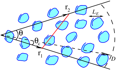
Figure 1: Schematic view of the turbulent field and the underlying geometry. At small angles, $\theta<\theta_{c}=L_{E}/D$, there are correlated fluctuations along the entire length of the lines of sight. At large angles only neighboring structures contribute to correlations.

In this example the 3d correlation function is zero at large separations. In general, however, the fluctuations may be present on large scales as well. This is the case, e.g., when the Kolmogorov turbulence is contained not within the “bubbles” as above, but within long sheets or filaments. When substantial power is present in fluctuations up to the largest scales, the correlation length may diverge.

Three-dimensional power spectrum of the magnetic field fluctuations, ${\cal B}(q)$, and the corresponding 3d correlation function are not measured directly. Instead, one measures the parameters of the two-dimensional angular correlation function $K(\theta)$ of some physical observable which can be, e.g., the intensity of the polarized synchrotron radiation or Faraday rotation measure along different directions, see Sect. III for examples. For such observables the relation between 3d correlation function and the angular correlation function involves integration along the line of sight as illustrated in Fig. 1. For example, in the case of Faraday rotation measure of extragalactic sources such relation reads

$$K(\theta)\propto\int_{0}^{D}dr_{1}dr_{2}\;\xi_{\rm RM}^{~{}}(|\bf{r}_{1}-\bf{r}_{2}|).$$ (12)

The directly measurable quantities are the structure function

$$\frac{1}{2}\,S(\theta)=K(0)-K(\theta),$$ (13)

and the two-dimensional power spectrum $C_{l}$ which at small angles is related to $K(\theta)$ by the Hankel transform

$$K(\theta)=\frac{1}{2\pi}\int_{0}^{\infty}C_{l}\,{\rm J_{0}}(l\theta)\;ldl.$$ (14)

Here the multipole $l$ corresponds to a typical angular scale of $\theta=\pi/l$.

In the case of the power-law behavior of the power spectrum, Eq. (7), both $S(\theta)$ and $C_{l}$ also follow power laws, $S(\theta)\propto\theta^{\beta}$ and $C_{l}\propto l^{-\gamma}$. In a certain range of $\alpha$ (see Appendix A for details) the three exponents are related as

$$\beta=\alpha,$$ (15)

$$\gamma=\alpha+2.$$ (16)

Eq. (15) is valid when $0<\alpha<2$. When the correlation length is finite, $K(\theta)\rightarrow 0$ at sufficiently large angles, and the structure function approaches constant (cf. Eq. (13)). Therefore, $\beta_{1}=0$ for any negative $\alpha_{1}$. On the other hand, at negative $\alpha$ the relation (16) holds. Making use of these two relations, the exponent $\alpha$ can be deduced from the observable quantities $\beta$ and $\gamma$. However, systematic observational effects (e.g., Faraday depolarization and finite beam width in the case of polarized synchrotron radiation) should be absent or accounted for.

The momentum scale $q_{c}$ at which the break in ${\cal B}(q)$ occurs is not observed directly either. Instead, one observes the break in the power-law behavior of $S(\theta)$ at some angular scale $\theta_{c}$ (or the break of $C_{l}$ at some multipole $l_{c}$). The scale $q_{c}$ can be estimated using the relation $l_{c}=Dq_{c}/2$, or

$$q_{c}=\frac{2\pi}{\theta_{c}D}\;,$$ (17)

see Appendix A. These relations involve another unknown parameter, the propagation distance in the magnetic field, $D$. Fortunately, in the expression for the cosmic ray deflections $q_{c}$ and $D$ enter as the product $q_{c}D$, so the result can be conveniently expressed in terms of the observable parameter $\theta_{c}$.

In the model of Fig. 1, the structure function at small angular scales $\theta<\theta_{c}=L_{E}/D$ should reflect Kolmogorov turbulence, $\beta_{2}=5/3$. On larger angular scales the structure function should gradually become flat, $\beta_{1}\rightarrow 0$. The correlation function in this case decays on large scales as $K(\theta)\propto\theta^{-1}$, which corresponds to $C_{l}\propto l^{-1}$ Cho:2002qk . In other words, existence of small (compared to $D$) correlation length corresponds to $\beta_{1}=0$ and $\gamma_{1}=1$.

III Observations of random component of GMF

Current knowledge of the Galactic magnetic field is based on: (i) Faraday rotation measurements of Galactic and extragalactic radio sources, (ii) starlight polarization data, and (iii) observations of diffuse Galactic synchrotron emission. Different methods are sensitive to the magnetic field in regions with different physical conditions. Faraday rotation is sensitive to a field in a warm ionized medium, stellar polarization measurements sample the field in regions occupied by interstellar dust grains, while synchrotron radiation originates from regions containing fast electrons.

Faraday rotation measure (RM) is sensitive to the projection of the magnetic field on the line of sight. The field direction along the line of sight is given by the sign of RM. The magnitude of the random field $B_{r}$ can be estimated by analyzing the deviations of RM from the uniform field along different directions.

Stellar and synchrotron polarization data contain information about the field perpendicular to the line of sight. This property is convenient for our purposes since the plane-of-the-sky component of the magnetic field determines also the deflections of UHECR primary particles. The ratio of the amplitudes of the random to the uniform magnetic field components can be estimated along a single direction. To extract the power spectrum one has to study angular correlation function of the polarization data.

III.1 The relative strength of uniform and random fields

Synchrotron emission. The total magnetic field strength is related to the synchrotron emissivity, while the polarization of the Galactic diffuse synchrotron background offers a method for determining the ratio of uniform to random field strengths. Namely, the observed fractional polarization $p_{\rm obs}$ along a given direction obeys Ginzburg

$$\frac{p_{\rm obs}}{p_{\rm max}}=\frac{B^{2}_{u,\bot}}{B^{2}_{u,\bot}+B^{2}_{r,\bot}}\;,$$ (18)

where the subscript $\bot$ on $B_{u}$ and $B_{r}$ refers to the plane-of-the-sky components of uniform and random field, respectively. In Eq. (18) $p_{\rm max}$ is the fractional polarization that would be observed for a perfectly uniform field, $p_{\rm max}\approx 0.72$. The fractional polarization of $p_{\rm obs}\approx 35\%$ was found in Ref.  Spoelstra to be a typical maximum for our Galaxy. This implies

$$B_{u,\bot}/B_{r,\bot}\approx 1\;.$$ (19)

Note that this ratio depends upon direction. For instance, in the direction of the Galactic anti-center $p_{\rm obs}\approx 20\%$ (being averaged over $-20^{\circ}<b<20^{\circ}$), which corresponds to $B_{u,\bot}/B_{r,\bot}\approx 0.62$. The typical coherence length was estimated in Ref. Spoelstra to be less than $75$ pc, while the distance to the region where polarized emission originates was found to be about $\sim 0.5$ kpc.

Starlight polarization. Polarization in starlight appears because of selective absorption by interstellar dust grains whose minor axis is aligned with the magnetic field $\bf{B}$. The same expression, Eq. (18), is valid for the starlight polarization data as well (with $p_{\rm max}$ being related to dust extinction). The resulting magnitude of the random component of magnetic field derived from the starlight polarization data is consistent with Eq. (19). For example, the estimate of Ref. Fosalba:2001wr reads $B_{u,\bot}/B_{r,\bot}\approx 0.8$.

Faraday rotation. Unlike polarization data, the Faraday rotation measure is sensitive to the magnetic field component parallel to the line of sight. Another disadvantage of this method is that it does not allow to find the ratio of random to uniform components of the magnetic field along a given direction. However, this information can be extracted from the residuals of a fit to a uniform field provided RMs in many neighboring directions are known. For instance, such kind of study for a particular region of the sky of about $10^{\circ}\times 10^{\circ}$ centered at $(l,b)\approx(140^{\circ},-40^{\circ})$ was carried out in Ref. Minter . It was found that $B_{r}\approx B_{u}$, in agreement with Eq. (19).

III.2 The power spectrum of magnetic field fluctuations

Synchrotron emission. The statistical properties of polarized synchrotron emission depend upon direction on the sky and are different for different observables. In Ref. Giardino:2002qi the angular power spectra (APS) of the Parkes survey of the Southern Galactic plane at 2.4 GHz were analyzed. It was found that in the multipole range $40<l<250$ ($0.7^{\circ}<\theta<5^{\circ}$) the APS of $E$ and $B$ components of the polarized signal has the slope $\gamma\approx 1.5$, and the power spectrum of polarization angle corresponds to $\gamma\approx 1.7$. Similar results were found in Refs. Bruscoli:2002fp ; Baccigalupi:2000pm for other Galactic latitudes. In particular, while being close to $1.5$ on average, the slopes of $E$ and $B$ components in the multipole range $l<1000$ ($\theta>10^{\prime}$) were found Bruscoli:2002fp to be in the range $1<\gamma<2.7$ depending on the particular region of the sky and the survey used.

Negative values of $\alpha$ (derived with the use of Eq.(16), if applicable) indicate that in many sky patches the correlation length of magnetic field may be small.

Starlight polarization. The angular power spectrum of the starlight polarization for the Galactic plane data ($|b|<10^{\circ}$) is consistent with $\gamma\approx 1.5$ for all angular scales $\theta>10^{\prime}$ (or $l<1000$), see Ref. Fosalba:2001wr .

Faraday rotation. Structure functions of the rotation measure of extragalactic radio sources were studied in Refs. Simonetti1 ; Simonetti2 ; Minter ; Clegg ; Sun:2004mt . Three different sky patches were considered in Ref. Simonetti1 . In two patches the index $\beta_{1}$ of the structure function of rotation measure was found to be consistent with zero on large angular scales $>2^{\circ}$, while in the third positive $\beta$ was observed. There is a clear drop in the structure function on small angular scales $\theta<0.1^{\circ}$, Simonetti1 ; Simonetti2 . Therefore, the break in the spectrum has to be at angular scales $0.1^{\circ}<\theta_{c}<2^{\circ}$ ($\theta_{c}$ cannot be quantified more precisely as there are no data points at these intermediate angular scales).

In Ref. Sun:2004mt shallow (with $\beta_{1}<0.3$) structure functions in several sky regions near the Galactic plain were found over the range $0.3^{\circ}<\theta_{c}<10^{\circ}$. Similar result was obtained in Ref. Clegg .

Minter and Spangler Minter have studied structure functions of RM from polarized extragalactic sources for a particular region with previously mapped emission measure of warm ionized medium. In this paper fluctuations in electron density were factored out and the power spectrum of fluctuating magnetic field was determined. The spectrum of random magnetic field derived in Ref. Minter can be parametrized by Eq. (8) with $A\approx 4.5\times 10^{-2}\;\mu G^{2}$. At large scales the angular structure function is consistent with the two-dimensional turbulence, $\alpha_{1}=2/3$, while at small scales $q>q_{c}$ the spectrum coincides with the Kolmogorov turbulence $\alpha_{2}=5/3$. The break in the spectrum occurs at $\theta_{c}\sim 0.07^{\circ}$ which corresponds to $2\pi/q_{c}\approx 3.6$ pc assuming $D=3$ kpc. With the parameters found in Ref. Minter , Eq. (9) gives $B_{r}\approx 1.6\;\mu G$. Note that for the uniform component of the magnetic field in the same region one has $B_{u}\approx 2.2\;\mu G$ and $B_{u,||}\approx-0.8\;\mu G$. The slope of $\alpha_{1}=2/3$ was measured up to $2\pi/q\sim 80$ pc. Thus, in this particular sky patch the correlation length of magnetic field fluctuations either diverges or is larger than 80 pc.

Power spectra and the structure functions of the rotation measure of the diffuse Galactic polarized radio background in several sky patches near the Galactic plain were studied in Ref. Haverkorn:2003ad . Angular power spectra show a spectral index $\gamma_{1}\approx 1$, while the structure functions are approximately flat, $\beta_{1}\approx 0$ in the range $0.1^{\circ}<\theta<10^{\circ}$. This is indicative of the field uncorrelated on large scales. The structure functions may show a break at $\theta_{c}$ close to $0.3^{\circ}$, which is at the same spatial scales ($\approx 3.9$ pc assuming a path length of 600 pc) as a break in the structure function in the RMs of extragalactic sources of Ref. Minter . Note that the RM of extragalactic sources probes the complete line of sight through the Galaxy, whereas, as a result of depolarization, the synchrotron emission observed at low frequencies only probes the nearby interstellar medium. In a similar study Haverkorn:2004fw in anther sky region, a shallow structure function of the rotation measures was found, $\beta_{1}\approx 0.2$ for $4^{\prime}<\theta<5^{\circ}$, while at smaller angular scales the structure function steepens.

IV UHECR deflections in the random magnetic field

In this section we show that the knowledge of the ratio $B_{u,\bot}/B_{r}$, the exponents $\alpha_{1}$ and $\alpha_{2}$, and the angular scale $\theta_{c}$ is sufficient to quantify the spread of deflections of UHECR primaries caused by the random component of GMF. As we have seen in Sect. III.1, the existing observations suggest that the magnitudes of the random and uniform components of GMF are comparable. In what follows it will be convenient to normalize the deflection due to the random field to the deflection $\delta_{u}$ which would occur in the uniform field over the same distance and at the same particle energy and charge. After traveling the distance $D$ in a uniform magnetic field, a particle with the electric charge $Ze$ and energy $E$ is deflected by an angle

$$\delta_{u}={ZeD\over E}\,B_{u,\bot}\;.$$ (20)

This has to be compared to the mean square deflection angle $\delta_{r}$ in the random component of the Galactic magnetic filed.

IV.1 Mean square deflection in terms of magnetic field power spectrum

Deflections of UHECR primaries by random magnetic field were studied in many papers, see e.g. Refs. Berezinsky:1989ji ; Blasi:1998xp ; Sigl:1998dd ; Achterberg:1999vr ; Stanev:2000fb ; Casse:2001be ; Yoshiguchi:2002rb ; Aloisio:2004jd . However, usually the main focus is the diffusive regime in the extra-galactic magnetic field. Deflections in the turbulent component of GMF were studied in Refs. Harari:2002dy ; Harari:2002fj , with the emphasis on the possibility of magnetic field reconstruction with future high statistics cosmic ray data. A generic turbulent component of GMF with a simplifying assumption of a cell-like structure was also included in the Monte-Carlo simulations of Ref. Prouza:2003yf . To our knowledge, estimates of UHECR deflections in the random field based on measurements of the MF power spectra in specific sky patches do not exist in the literature. The UHECR deflections in the situation when the coherence length is not small (which might be relevant for the case of realistic GMF) was not studied in detail either.

Propagation of UHECR primaries in the Galaxy is quasi-rectilinear, with typical deflection angles not exceeding $10^{\circ}-20^{\circ}$ even for lowest energies. The contribution of turbulent field in these deflections is expected to be even smaller. Therefore, a ballistic approximation gives a good description of UHECR propagation. In this regime, the deflection angles are characterized by the following line integrals,

$$\delta_{i}={Ze\over E}\int_{0}^{D}dz\;\epsilon_{ik}B_{k}(z)\;,$$ (21)

where the axis $z$ is chosen along the particle trajectory and indices $i,k=1,2$ label two orthogonal directions. The mean square deflections are

$$\delta_{r}^{2}\equiv\langle\delta_{i}\delta^{i}\rangle={Z^{2}e^{2}\over E^{2}}\int\!\!\!\int_{0}^{D}dz\,dz^{\prime}\;\epsilon_{ik}\epsilon_{jp}\langle B_{k}(z)B_{p}(z^{\prime})\rangle\;.$$ (22)

Here the average is taken over the ensemble of different realizations of the turbulent magnetic field $B_{a}(x)$. For a statistically homogeneous random field the correlator in Eq. (22) is the function of $r=z^{\prime}-z$

$$\epsilon_{ik}\epsilon_{jp}\langle B_{k}(z)B_{p}(z^{\prime})\rangle=\xi_{11}(r)+\xi_{22}(r)\equiv\xi_{\bot}(r)\;,$$ (23)

where $\xi_{ii}(r)\equiv\langle B_{i}(z)B_{i}(z+r)\rangle$ (no summation over $i$). Using Eq. (3) which enforces the divergence-free constraint one finds

$$\xi_{\bot}(r)=4\pi\int_{0}^{\infty}{dq\,\over q}{\cal B}(q)\left[\frac{\sin(qr)}{qr}+\frac{\cos(qr)}{q^{2}r^{2}}-\frac{\sin(qr)}{q^{3}r^{3}}\right]\;.$$

This relation implies

$$\int_{0}^{\infty}dr\;\xi_{\bot}(r)=\frac{1}{2}\int_{0}^{\infty}dr\;\xi(r)\;.$$ (24)

Note that the assumption of chaotically oriented magnetic cells, which is often made, would give instead $\xi_{\bot}(r)=(2/3)\;\xi(r)$. However, this assumption is inconsistent with the divergence-free nature of the magnetic field.

Changing variables in Eq. (22) from $z$, $z^{\prime}$ to $r$ and $u=(z+z^{\prime})$ one obtains

$$\delta_{r}^{2}={2Z^{2}e^{2}\over E^{2}}\;B^{2}_{r}\int_{0}^{D}du\int_{0}^{u}dr\;\frac{\xi_{\bot}(r)}{\xi(0)}\;,$$ (25)

where Eq. (5) was used. It is convenient to represent the result as a ratio of rms deflections in random field to the deflection in the uniform field $\delta_{u}$ given by Eq. (20). Thus, we arrive at Eq. (2) where the dimensionless factor $R$ is

$$R^{2}\equiv\frac{2}{D^{2}}\;\int_{0}^{D}du\int_{0}^{u}dr\;\frac{\xi_{\bot}(r)}{\xi(0)}\;.$$ (26)

This factor varies between zero and one.

If the correlation length $L_{c}$ defined by Eq. (6) is much smaller than the propagation distance $D$, the upper limit in the integral over $r$ can be extended to infinity. One then finds

$$R^{2}=\frac{L_{c}}{D}\;.$$ (27)

In the general case, the expression Eq. (26) can be brought to the form

$$R^{2}=\frac{4\pi}{D\xi(0)}\int_{0}^{\infty}{dq\,\over q^{2}}{\cal B}(q)\,f(Dq)\;,$$ (28)

where

$$f(x)={\rm Si}(x)+\frac{\cos x}{x}-\frac{\sin x}{x^{2}}\;,$$ (29)

and  ${\rm Si}(x)=\int_{0}^{x}dy\,\sin(y)/y$  is the integral sine function. At small arguments the function $f(x)$ grows linearly as $f(x)=2x/3+O(x^{3})$, while at $x\mathrel{\raisebox{-2.36806pt}{\hbox to0.0pt{$\sim$\hss}}\raisebox{1.72218pt}{$>$}}2\pi$ it rapidly converges to the asymptotic value $\pi/2$.

IV.2 Mean square deflections in the random component of GMF

With the assumption that the power-law spectrum of the turbulent magnetic field is given by Eq. (8), as supported by the existing observations, Eq. (28) gives

$$R^{2}=\frac{(\alpha_{2}-1)(1-\alpha_{1})}{(\alpha_{2}-\alpha_{1})}\;\times$$ (30)

$$\left[(Dq_{c})^{\alpha_{1}-1}\,\int_{0}^{Dq_{c}}{dyf(y)\over y^{1+\alpha_{1}}}+(Dq_{c})^{\alpha_{2}-1}\,\int_{Dq_{c}}^{\infty}{dyf(y)\over y^{1+\alpha_{2}}}\right]\;,$$

where $f(y)$ is defined in Eq. (29). As one can see, the final result depends on the product $Dq_{c}$. Therefore, with the use of Eq. (17) it can be rewritten in terms of the single directly observable scale $\theta_{c}=2\pi/Dq_{c}$.

In the case $Dq_{c}\gg\pi$ and $\alpha_{1}<0$ (when both integrals are saturated at $y=Dq_{c}$), we recover Eq. (27),

$$R=\sqrt{\frac{L_{c}}{D}}=\sqrt{\frac{\theta_{c}}{4}\,\frac{(\alpha_{1}-1)(\alpha_{2}-1)}{\alpha_{1}\alpha_{2}}}.$$ (31)

For $\alpha_{1}$ varying within $0.2<\alpha_{1}<0.8$ and $\alpha_{2}=5/3$ (which corresponds to the Kolmogorov turbulence), there exists an approximate analytic expression for $R$ which holds with an accuracy of about 10%,

$$R\approx(Dq_{c})^{(\alpha_{1}-1)/2}=(\theta_{c}/2\pi)^{(1-\alpha_{1})/2}\;.$$ (32)

In the general case the factor $R$ has to be calculated numerically. Its dependence on $\alpha_{1}$ for $\alpha_{2}=5/3$ in three cases $\theta_{c}=6^{\circ}$, $\theta_{c}=0.6^{\circ}$ and $\theta_{c}=0.06^{\circ}$ is shown in Fig. 2 by the dotted, dashed and solid lines, respectively. We recall now that in many “low” resolution all-sky studies the steepening of APS is not detected, up to large multipoles, $l\sim 1000$. This suggests that $\theta_{c}<10^{\prime}$ and the dashed line in Fig. 2 may serve as an upper limit for the factor $R$.

The labeled data-points in Fig. 2 represent the data based on the Faraday rotation measurements. The corresponding survey regions are shown in Fig. 3 as colored patches labeled in the same way as the data-points by A (Ref. Minter ), B1,B2 (Refs. Simonetti1 ; Simonetti2 ), C1,C2 (Ref. Haverkorn:2003ad ), D (Ref. Haverkorn:2004fw ) and E1,E2,E2 (Ref. Sun:2004mt ). Only in the region A the transition to the Kolgomogorov turbulence was detected at the scale $\theta_{c}\sim 0.07^{\circ}$. Though in some other regions an indication for the break was observed, the transition to the spectra with $\alpha_{2}>1$ was not established. The corresponding limits on $\theta_{c}$ are shown as downward arrows. As explained in the Appendix A, any negative $\alpha$ corresponds to $\beta=0$ in the structure functions. Therefore, we plot data-points with $\beta=0$ as downward arrows at $\alpha_{1}=0$ turning to the left (pointing to the region of negative $\alpha_{1}$). Finally, in the regions C1,C2 both the structure functions and the APS of rotation measure were obtained Haverkorn:2003ad resulting in $\beta\approx 0$ and $\gamma\approx 1$. This allows to specify $\alpha_{1}$ in these regions as $\alpha_{1}\mathrel{\raisebox{-2.36806pt}{\hbox to0.0pt{$\sim$\hss}}\raisebox{1.72218pt}{$<$}}-1$.

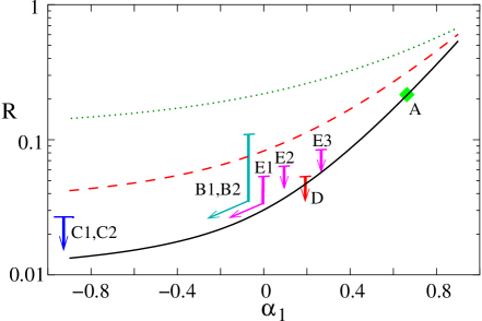
Figure 2: The coefficient R as a function of $\alpha_{1}$ is shown by dotted, dashed and solid curves for $\theta_{c}=6^{\circ},~{}0.6^{\circ}$ and $0.06^{\circ}$ respectively. The data-points correspond to the APS derived for sky regions A-E, as discussed in the text. These regions are displayed in Fig. 3.

Small observed values of (or upper limits on) $\theta_{c}$ indicate that either the scale $2\pi/q_{c}$ is small, or the extent of GMF along given direction, $D$, is large. In either case the resulting coefficient $R$ is small, $0.02<R<0.2$. Note that the application of Eq. (2) to the directions along the Galactic plane should be done with care. Namely, deflections in the regular field cannot be approximated by a simple relation (20), but should be replaced by the integral along the line of sight. Existing field reversals can diminish deflections in the regular field considerably.

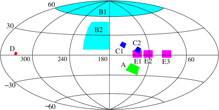
Figure 3: Regions A-E in Galactic coordinates where the break in the APS was detected. Corresponding values of $R$ for these regions are shown as data-points in Fig. 2.

V Conclusions

Deflections of UHECR in the random component of the Galactic magnetic field are usually discussed in the limit when the correlation length $L_{c}$ is much smaller than the propagation distance $D$. However, even in this limit both the correlation length and the propagation distance in GMF (and therefore typical deflections) vary with direction. Moreover, the existing GMF data suggest that the assumption of small correlation length may not be valid uniformly all over the sky.

We have calculated deflections in a more general approach which does not require correlation length to be small and relies directly on the spectrum of GMF fluctuations measured in a relatively small patch of the sky. Our method therefore automatically takes into account variations of the GMF characteristics with direction. We have shown that the ratio of the deflections in the random and uniform components of GMF, Eq. (2), is expressed in terms of the factor $R$ which depends on the spectrum of the magnetic field fluctuations as given by Eq. (28). For the power-law spectrum with a single break the factor $R$ can be written as a function of one directly observable parameter $\theta_{c}$, the angular scale of the break in the relevant structure function. In the case of a small correlation length one finds $R\sim\sqrt{\theta_{c}}$.

Using the measurements of the GMF power spectrum in the sky regions where it is available, we have shown that the deflections in the random component are small, $0.03-0.3$ of the deflections in the uniform field, see Fig. 2. This is sufficiently small not to preclude identification of sources of UHECR using methods of Refs. Tinyakov:2001nr ; Tinyakov:2003nu ; Tinyakov:2001ir . For instance, the deflection of a proton with energy $E=4\times 10^{19}$ eV due to the random component of GMF is expected to be about $0.2^{\circ}-1.5^{\circ}$ depending on the direction. This is below the resolution of the AGASA experiment, but can be above the resolution of the HiRes detector in the stereo mode and the expected resolution of the Pierre Auger experiment. Thus, the detailed study of the random component of GMF is particularly important for the interpretation of data which will be collected by the new generation of UHECR experiments. To this end, the all-sky map of the essential parameters determining the power spectra of GMF is highly desirable. These maps may be obtained from the measurements of Faraday rotation and maps of diffuse polarized synchrotron Galactic emission.

Appendix A Angular structure functions, angular power spectrum and underlying 3D power spectrum.

In this section we derive Eqs. (15)–(17). These equations are valid for a large class of observables including Faraday rotation measures. To simplify the presentation we derive them in the case when the correlation function is given by equation (4).

The relation between 3d correlation function and angular correlation function involves the integration along the line of sight,

$$K(\theta)=\int_{0}^{D}r_{1}^{a}dr_{1}r_{2}^{a}dr_{2}\;\xi(|\bf{r}_{1}-\bf{r}_{2}|),$$ (33)

where $\theta$ is the angle between the vectors ${\bf r_{1}}$ and ${\bf r_{2}}$ and $a$ takes the values $0$ and $2$ in the case of point sources and diffuse radiation, respectively. We concentrate in what follows on the case $a=0$ relevant for all points in Fig. 2 except $C_{1,2}$ and $D$.

Introducing the variables $v\equiv r_{1}-r_{2}$ and $y\equiv(r_{1}+r_{2})/2$ and taking the limit of small angles one can write Eq. (33) as follows,

$$K(\theta)=4\int_{0}^{D/2}dy\int_{0}^{2y}dv\;\xi(\sqrt{v^{2}+y^{2}\theta^{2}}).$$ (34)

Integration over $dv$ gives

$$K(\theta)=16\pi\int_{0}^{D/2}dy\int_{0}^{\infty}\frac{dq}{q^{2}}{\cal B}(q)$$

$$\times\left[\frac{\pi}{2}{\rm J_{0}}(yq\theta)-\frac{\pi}{2}+{\rm Si}(2yq)\right],$$ (35)

where ${\rm J_{0}}$ and ${\rm Si}~{}$ are the Bessel and integral sine functions, respectively. According to definition (13), this relation gives for the structure function $S(\theta)$:

$$S(\theta)=16\pi^{2}\int_{0}^{D/2}dy\int_{0}^{\infty}\frac{dq}{q^{2}}{\cal B}(q)\left[1-{\rm J_{0}}(yq\theta)\right].$$ (36)

Let us assume that ${\cal B}$ is a broken power law, Eq. (8). Then the structure function is also a broken power law behaving as $S\propto\theta^{\beta_{1}}$ and $S\propto\theta^{\beta_{2}}$ below and above the angular scale $\theta_{c}$, respectively. The exponents $\beta_{i}$ are related to exponents $\alpha_{i}$ in Eq. (8) as follows,

$$\beta = 2~{}~{}~{}~{}{\rm if}~{}~{}~{}~{}\alpha>2,$$

$$\beta = \alpha~{}~{}~{}~{}{\rm if}~{}~{}~{}~{}0<\alpha<2,$$

$$\beta = \,0~{}~{}~{}~{}{\rm if}~{}~{}~{}~{}\alpha<0.$$ (37)

The break occurs at

$$\theta_{c}=\frac{2\pi}{q_{c}D}.$$ (38)

The angular power spectrum, $C_{l}$, and the angular correlation function at small angles are related by the Hankel transform, Eq. (14). If ${\cal B}$ is given by the power law (8) with $\alpha_{1}<0$ (i.e., the correlation length converges), the integral in Eq. (35) is saturated in the region $yq\gg 1$. In this region ${\rm Si}(2yq)\rightarrow{\pi}/{2}$; therefore, the last two terms in Eq. (35) can be neglected. (This holds whenever the correlation length is much smaller $D$ and the integration over $dv$ in Eq. (34) can be extended to infinity.) Comparison of Eqs. (35) and (14) gives then

$$C^{~{}}_{l}=\frac{16\pi^{3}}{l^{3}}\int_{0}^{D/2}{\cal B}\left(\frac{l}{y}\right)\,y\,dy.$$ (39)

Note that Eq. (39) is generalized trivially to the case of non-zero $a$ by replacing $ydy$ by $y^{1+2a}dy$. For a broken power-law behavior of ${\cal B}$, the angular power spectrum is also a broken power law,  $C_{l}\propto l^{-\gamma}$,  where the exponents $\gamma_{i}$ are

$$\gamma_{i}=\alpha_{i}+2$$ (40)

and the break occurs at $l_{c}=Dq_{c}/2$.

References

- (1) K. Dolag, D. Grasso, V. Springel and I. Tkachev, JETP Lett. 79 (2004) 583 [astro-ph/0310902] and astro-ph/0410419.
- (2) G. Sigl, F. Miniati and T. A. Ensslin, Phys. Rev. D 70 (2004) 043007 [astro-ph/0401084].
- (3) M. Simard-Normandin and P. P. Kronberg, Ap. J. 242 (1980) 74; R. J. Rand and A. G. Lyne, MNRAS 268 (1994) 497; J. L. Han and G. J. Qiao, Astron. Astrophys. 288 (1994) 759; J. P. Vallee, Ap. J. 454 (1995) 119; C. Indrani and A. A. Deshpande, New Astronomy 4 (1998) 33; J. L. Han, R. N. Manchester, and G. J. Qiao, MNRAS 306 (1999) 371; P. Frick, R. Stepanov, A. Shukurov and D. Sokoloff, Mon. Not. Roy. Astron. Soc. 325 (2001) 649; R. Beck, astro-ph/0310287.
- (4) T. Stanev, Astrophys. J. 479 (1997) 290 [arXiv:astro-ph/9607086].
- (5) P. G. Tinyakov and I. I. Tkachev, Astropart. Phys. 18 (2002) 165 [astro-ph/0111305].
- (6) D. S. Gorbunov, P. G. Tinyakov, I. I. Tkachev and S. V. Troitsky, Astrophys. J. 577 (2002) L93 [astro-ph/0204360].
- (7) M. Teshima et al., The Arrival Direction Distribution of Extremely High Energy Cosmic Rays Observed by AGASA. In proceedings of 28th International Cosmic Ray Conference (ICRC 2003), Tsukuba, Japan, pp. 437-440.
- (8) P. G. Tinyakov and I. I. Tkachev, Correlations and charge composition of UHECR without knowledge of galactic magnetic field. In proceedings of 28th International Cosmic Ray Conference (ICRC 2003), Tsukuba, Japan, pp. 671-674, astro-ph/0305363.
- (9) P. P. Kronberg, Rept. Prog. Phys. 57 (1994) 325.
- (10) D. Harari, S. Mollerach, E. Roulet and F. Sanchez, JHEP 0203 (2002) 045 [astro-ph/0202362].
- (11) D. Harari, S. Mollerach and E. Roulet, JHEP 0207 (2002) 006 [astro-ph/0205484].
- (12) S. L. Dubovsky, P. G. Tinyakov and I. I. Tkachev, Phys. Rev. Lett. 85 (2000) 1154; Z. Fodor and S. D. Katz, Phys. Rev. D 63 (2001) 023002; H. Yoshiguchi, S. Nagataki, S. Tsubaki and K. Sato, Astrophys. J. 586 (2003) 1211; P. Blasi and D. De Marco, Astropart. Phys. 20 (2004) 559; D. Harari, S. Mollerach and E. Roulet, JCAP 0405 (2004) 010; M. Kachelriess and D. Semikoz, arXiv:astro-ph/0405258.
- (13) V. S. Berezinsky, S. V. Bulanov, V. A. Dogiel, V. L. Ginzburg, and V. S. Ptuskin, Astrophysics of Cosmic Rays, Amsterdam: Elsevier, 1990.
- (14) E. Roulet, Int. J. Mod. Phys. A 19 (2004) 1133 [arXiv:astro-ph/0310367].
- (15) A. Minter and S. Spangler, Astrophys. J. 458 (1996) 194.
- (16) J. Cho and A. Lazarian, Astrophys. J. 575 (2002) L63 [arXiv:astro-ph/0205284].
- (17) V. L. Ginzburg and S.I. Syrovatskii, Ann. Rev. Astron. Astrophys. 3 (1965) 297.
- (18) T.A.T. Spoelstra, A&A 135 (1984) 238.
- (19) P. Fosalba, A. Lazarian, S. Prunet and J. A. Tauber, Astrophys. J. 564 (2002) 762 [astro-ph/0105023].
- (20) G. Giardino, A. J. Banday, K. M. Gorski, K. Bennett, J. L. Jonas and J. Tauber, A&A 387 (2002) 82 [astro-ph/0202520].
- (21) M. Bruscoli, M. Tucci, V. Natale, E. Carretti, R. Fabbri, C. Sbarra and S. Cortiglioni, New Astronomy, 7 (2002) 171 [astro-ph/0202389].
- (22) C. Baccigalupi et al., astro-ph/0009135.
- (23) J.H. Simonetti, J.M. Cordes and S.R. Spangler, Astrophys. J. 284 (1984) 126.
- (24) J.H. Simonetti and J.M. Cordes, Astrophys. J. 310 (1986) 160.
- (25) A. W. Clegg, J. M. Cordes, J. H. Simonetti and S. R. Kulkarni, Astrophys. J. 386 (1992) 143.
- (26) X. H. Sun and J. L. Han, astro-ph/0402180.
- (27) M. Haverkorn, P. Katgert and A. G. de Bruyn, Astron. Astrophys. 403 (2003) 1045 [astro-ph/0303644].
- (28) M. Haverkorn, B. M. Gaensler, N. M. McClure-Griffiths, J. M. Dickey and A. J. Green, astro-ph/0403655.
- (29) V. S. Berezinsky, S. I. Grigoreva and V. A. Dogel, Sov. Phys. JETP 69 (1989) 453 [Zh. Eksp. Teor. Fiz. 96 (1989) 798].
- (30) P. Blasi and A. V. Olinto, Phys. Rev. D 59 (1999) 023001 [astro-ph/9806264].
- (31) G. Sigl, M. Lemoine and P. Biermann, Astropart. Phys. 10, 141 (1999) [astro-ph/9806283].
- (32) A. Achterberg, Y. A. Gallant, C. A. Norman and D. B. Melrose, astro-ph/9907060.
- (33) T. Stanev, R. Engel, A. Mucke, R. J. Protheroe and J. P. Rachen, Phys. Rev. D 62 (2000) 093005 [astro-ph/0003484].
- (34) F. Casse, M. Lemoine and G. Pelletier, Phys. Rev. D 65, 023002 (2002) [astro-ph/0109223].
- (35) H. Yoshiguchi, S. Nagataki, S. Tsubaki and K. Sato, Astrophys. J. 586 (2003) 1211 [Erratum-ibid. 601 (2004) 592] [astro-ph/0210132].
- (36) R. Aloisio and V. Berezinsky, astro-ph/0403095.
- (37) M. Prouza and R. Smida, astro-ph/0307165.
- (38) P. G. Tinyakov and I. I. Tkachev, JETP Lett. 74 (2001) 445 [astro-ph/0102476].