Internal colour gradients for E/S0 galaxies in Abell 2218

Abstract

We determine colour gradients of $-0.15\pm 0.08$ magnitudes per decade in radius in F450W$-$F606W and $-0.07\pm 0.06$ magnitudes per decade in radius in F606W$-$F814W for a sample of 22 E/S0 galaxies in Abell 2218. These gradients are consistent with the existence of a mild ($\sim-0.3$ dex per decade in radius) gradient in metal abundance, (cf. previous work at lower and higher redshift for field and cluster galaxies). The size of the observed gradients is found to be independent of luminosity over a range spanning $M^{*}-1$ to $M^{*}+1.5$ and also to be independent of morphological type. These results suggest a fundamental similarity in the distributions of stellar populations in ellipticals and the bulges of lenticular galaxies. These results are not consistent with simple models of either monolithic collapse or hierarchical mergers.

1 Introduction

In Hubble’s (1936) classification scheme for galaxies, lenticular (S0) galaxies first appear as a transitional class between the ellipticals and the two branches (barred and unbarred) of the spirals, and, despite much evidence to the contrary, it has often been assumed that the Hubble ‘fork’ describes an evolutionary scheme. For instance, this assumption informs the popular idea that collisions of proto-disks in the early universe lead to the formation of elliptical galaxies or that quenching of star formation in field spirals as they fall into dense regions leads, by a variety of mechanisms, to their transformation into S0 galaxies. This process, first proposed by Larson, Tinsley & Caldwell (1980), has been invoked to account for the morphology-density relation of Dressler (1980) and the apparent blueing of the galaxy population in distant clusters (Butcher & Oemler 1984), and has stimulated considerable theoretical activity (see Pimbblet 2003 for a review).

Such processes modify the star formation history of the disk by removing the supplies of gas necessary to fuel further star formation. A sensitive test of this mechanism would therefore involve a comparison of the stellar populations of bulges and disks for elliptical, S0 and spiral galaxies. While the stellar content of galaxies cannot be resolved except for some of the nearest objects, the radial distributions of their stellar populations may be examined by means of colour gradients.

It has long been known that early-type galaxies exhibit negative colour gradients, in the sense of being bluer at larger radii (Franx, Illingworth & Heckman 1989, Peletier et al. 1990, Goudfrooij et al. 1994, Tamura et al. 1999, Saglia et al. 2000, Tamura & Ohta 2000, Hinkley & Im 2001, Idiart, Michard & de Freitas Pacheco 2002, Tamura & Ohta 2003). These gradients have been conventionally interpreted as representing gradients in mean metal abundance, as most local ellipticals also exhibit such gradients in the strength of metal absorption lines (Baum, Thomsen & Morgan 1986, Carollo, Danziger & Buson 1993, Davies, Sadler & Peletier 1993). However, this intepretation is vitiated by the existence of a strong degeneracy between age and metallicity in broadband colours as well as in most spectrophotometric indices (Worthey 1996). Nevertheless, colour gradients have considerable potential for constraining the history of star formation in distant galaxies, and for providing clues to their formation and evolution history.

One approach to breaking the age–metallicity degeneracy is to consider the evolution of colour gradients. This experiment has been attempted in a few distant clusters with rich populations of early-type galaxies. Saglia et al. (2000), Tamura & Ohta (2000) and La Barbera et al. (2003) have observed galaxies in clusters at $z\sim 0.4$ and studied the evolution of their colour gradients, concluding that the most likely explanation consists of a mild metal abundance gradient within a passively evolving stellar population formed at very high redshift.

However, because of the relatively limited number of galaxies and relatively poor resolution at these redshifts, even with Hubble Space Telescope (HST) imaging, Saglia et al. (2000), Tamura & Ohta (2000) and La Barbera et al. (2003) have not examined the dependence of colour gradients on galaxy luminosities and morphology and whether the disk and bulge components of galaxies have different gradients, and therefore different stellar populations. It is therefore useful to consider a somewhat lower-redshift target, where the galaxy population can be probed over a wider range of luminosities and where the higher spatial resolution (because of the lower distance) and smaller cosmological dimming allow more detailed studies of colour gradient evolution than has been possible (cf. Tamura & Ohta 2003 for a similar approach to the $z=0.03$ cluster Abell 2199).

In this paper we discuss a study of colour gradients in the $z=0.18$ cluster Abell 2218 from deep archival HST multicolour data. We describe the data and the analysis in the following section and present the main results. We discuss these results in the light of models of galaxy formation and, particularly, disk evolution. We adopt the concordance cosmological model with $\Omega_{M}=0.3$, $\Omega_{\Lambda}=0.7$ and H${}_{0}=70$ km s^-1 Mpc^-1.

2 Data analysis

Figure 1: Surface brightness profiles and colour gradients for galaxies in A2218 (as identified in the figure). In each figure panel (one per galaxy), the top panel shows the surface brightness profiles in $B^{\prime}$ (circles), $V^{\prime}$ (squares) and $I^{\prime}$ (triangles) plotted against $\log r$ (measured in arcseconds along the semi-major axis); the middle panel shows the colour distribution as a function of $\log r$ in $B^{\prime}-V^{\prime}$ (data points are the filled circles, error bars are the statistical error in the flux, the dashed lines show the effect of a $\pm 1\sigma$ error in subtracting the sky level, and the thick dashed line shows the best fitting straight line); the bottom panel is the same as the middle panel, but for $V^{\prime}-I^{\prime}$ and using squares. The open symbols in all panels show the surface brightness values and colours for points interior to $r=0.3^{\prime\prime}$ which were not used in the fit. Note that we refer to the $B^{\prime}$, $V^{\prime}$ and $I^{\prime}$ colours by their proper HST names, to avoid confusion for those who may wish to make use of these data (the actual profiles are available on request in machine-readable format).

Figure 1: (continued)

Figure 1: (continued)

Figure 1: (continued)

Figure 1: (continued)

The data consist of three archival images of the core of Abell 2218 taken by the HST with the Wide Field and Planetary Camera 2 (WFPC2) through filters F450W, F606W and F814W (PID: 8500; PI: Fruchter). For simplicity, we will refer to these bands as $B^{\prime}$, $V^{\prime}$ and $I^{\prime}$ in the remainder of this paper (we use prime symbols to distinguish the bands from the actual Johnson bands and to avoid confusion in the subsequent discussion). The total exposure times were 12000s, 10000s and 12000s respectively, with individual exposures being 1000s each. These images were retrieved as fully processed associations from the HST archive ( Micol, Bristow & Pirenne 1997). A more detailed description of this dataset is given by Smail et al. (2001).

We have selected a sample of 24 galaxies morphologically classified as E or S0 and spectroscopically confirmed to be cluster members (this information is taken from Smail et al. 2001). First, the mean sky was removed from the images using the IRAF task sky. For each galaxy we then derived surface brightness profiles using the IRAF task ellipse (Jedrzejewski 1987, Busko 1996), using $0.1^{\prime\prime}$ (1-pixel) sampling and 3$\sigma$ clipping to remove overlapping stars and galaxies. As our main interest in these data is to derive colour gradients, we forced the isophotes in $V^{\prime}$ and $I^{\prime}$ to be evaluated at the same radius (measured along the semi-major axis) as in the $B^{\prime}$ image (which is the one with the lowest signal to noise) by using the ‘inellip’ option in ellipse. The isophote centres were left free to be recentered for each image, to avoid the effect of minor misalignments between the HST images in the different bands.

In some cases, galaxies lie in the envelope of other bright galaxies or overlap with nearby galaxies (especially the two giant ellipticals but also in a few other cases). In these cases, we have modelled the ‘contaminating’ object using the IRAF task bmodel and removed it from the image. We then computed new isophotes for the galaxies. In most cases, this appears to make no difference, at least to the level of producing colour gradients different by more than the statistical and systematic errors. However, galaxies # 292 and #298 appear to be significantly affected by the envelopes (and, in the case of # 292 proximity to the edge of the detector) of their neighbouring galaxies. Because of this we decided to exclude these two galaxies from our analysis. In other cases, such as # 205 and # 634, modelling shows that the profiles are not being affected by proximity to a bright neighbour and that ellipse has appropriately removed the contaminating object from the profile..

For each data point, two sources of error contribute; using the terminology of Saglia et al. (2000) these are: a statistical error, which is the uncertainty, returned by ellipse in measuring the mean flux along each isophote and a systematic error, reflecting the uncertainty in measuring and subtracting the mean sky level. We estimated this latter component in the following way: for each of the individual 1000s exposures in each band, we calculate the mean sky using sky. This yields 12, 10 and 12 sky estimates in $B^{\prime}$,$V^{\prime}$ and $I^{\prime}$. The error in the mean sky is then computed by jackknife resampling of these sky estimates.

We calibrate the data on to the Vega system, using the zeropoints provided by Holtzman et al. (1995). At each isophote semi-major radius we then compute the resulting colour as a function of radius.

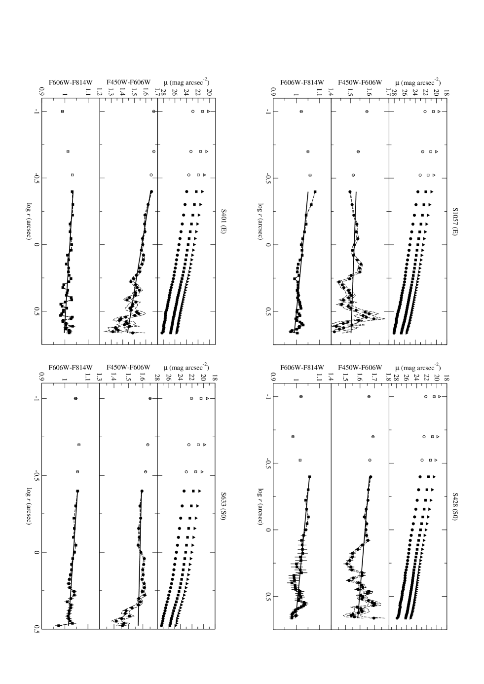
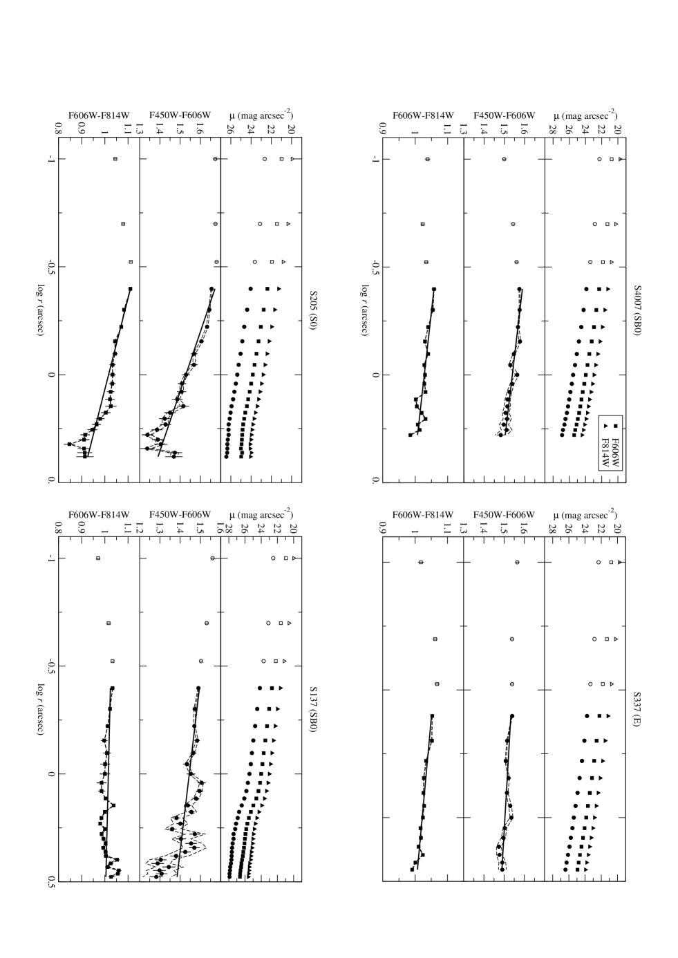
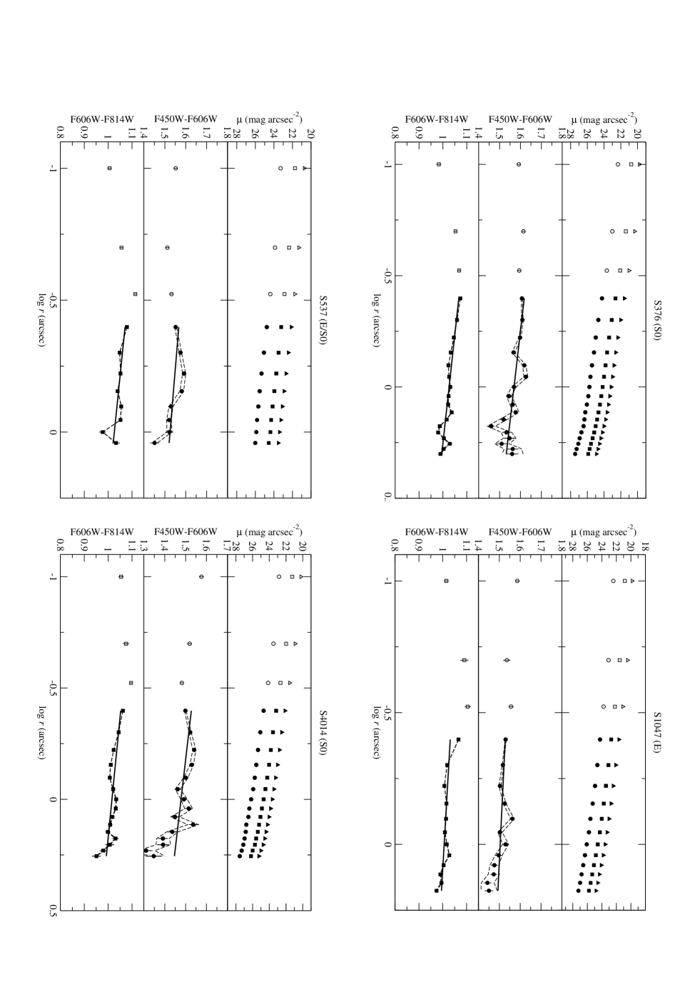
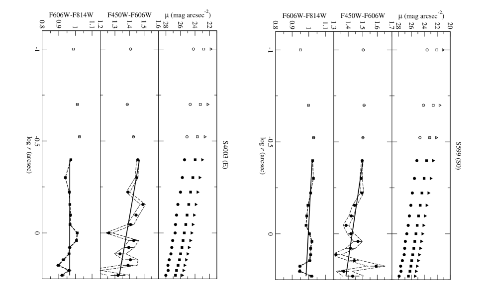
We measured the point spread function using non-saturated stars in our images. There are, unfortunately, only a few such stars but the full width at half maximum appears to be a consistent $0.15^{\prime\prime}$ in all bands, suggesting that differences in the point spread function do not affect the derivation of colour gradients. Inspection of the surface brightness profiles in Figure 1, shows some deviation from the profile expected for a de Vaucouleurs profile in the inner two or three points. For this reason, we decide to fit to the points with $r>0.3^{\prime\prime}$ in order to avoid any residual effects due to small differences in the point spread function.

The colour gradients are then derived by fitting the data (colour vs. logarithm of the radius measured along the semi-major axis) with a weighted linear least squares regression, where the weights are the statistical errors of the colours (added in quadrature). The fits are carried out to either the radius at which the quadratic sum of statistical and systematic errors exceeds 10% or to the radius at which ellipse stopped integrating the surface brightness profile (even if the errors are smaller than 10%). We also estimate the colour gradient only over the range defined by our worst colour ($B^{\prime}-V^{\prime}$), for consistency. The statistical error on the fit slope and intercept is derived from the error in the fit to the data, while the systematic error is determined by carrying out a new fit to the data points, after adding and subtracting the $\pm 1\sigma$ error in the sky level.

Figure 1 shows the surface brightness profiles in all three filters and the colour gradients in $B^{\prime}-V^{\prime}$ and $V^{\prime}-I^{\prime}$, plotted against $\log r$, for all 22 galaxies. The surface brightness profiles and colour profiles are plotted over the range $r=0$ to the largest radius used in fitting the colour gradients. As for points interior to $0.3^{\prime\prime}$, which are not used in fitting, some galaxies show colours consistent with the extrapolated fits, while in some other cases it is possible that the galaxies contain ‘cores’ with flatter colours. However, this is difficult to ascertain without data at better resolution.

The major contribution to the error budget comes, not unexpectedly, from the $B^{\prime}$ band, where the WFPC2 camera is less efficient and the galaxies are fainter (as it corresponds to the rest-frame $U$). We tabulate the results in Table 1. This shows, in column order, the galaxy ID, morphology and $K$ band luminosity (from Smail et al. 2001), the $B^{\prime}-V^{\prime}$ colour gradient with its statistical and systematic error, and the and $V^{\prime}-I^{\prime}$ colour gradient with its statistical and systematic error (derived as described above). The mean gradients are $\Delta(B^{\prime}-V^{\prime})/\Delta\log r=-0.14\pm 0.08$ for Es and $-0.16\pm 0.09$ for S0s and $\Delta(V^{\prime}-I^{\prime})/\Delta\log r=-0.06\pm 0.04$ for Es and $-0.08\pm 0.06$ for S0s.

Table 1: Colour gradients

ID	Morphology	$K$	$\Delta(B^{\prime}-V^{\prime})/d\log r$	$\sigma_{stat}$	$\sigma_{sys}$	$\Delta(V^{\prime}-I^{\prime})/d\log r$	$\sigma_{stat}$	$\sigma{sys}$
301	cD	13.19	$-$0.059	0.002	0.016	$-$0.006	0.001	0.001
307	E	13.77	$-$0.124	0.004	0.017	$-$0.042	0.002	0.001
280	SB0a	14.37	$-$0.180	0.006	0.024	$-$0.092	0.004	0.002
315	E	14.55	$-$0.247	0.007	0.022	$-$0.064	0.006	0.002
1057	E	14.57	$-$0.026	0.006	0.042	$-$0.056	0.002	0.004
428	S0	14.60	$-$0.076	0.006	0.040	$-$0.056	0.003	0.002
401	E	14.85	$-$0.188	0.005	0.044	$-$0.036	0.002	0.003
633	S0	14.88	$-$0.026	0.001	0.025	$-$0.045	0.006	0.002
4007	SB0	15.17	$-$0.125	0.011	0.030	$-$0.075	0.007	0.002
337	E	15.20	$-$0.073	0.009	0.016	$-$0.072	0.005	0.001
205	S0	15.21	$-$0.361	0.015	0.020	$-$0.237	0.011	0.001
137	SB0	15.52	$-$0.126	0.011	0.062	$-$0.022	0.005	0.006
376	S0	15.54	$-$0.123	0.012	0.032	$-$0.102	0.006	0.002
1047	E	15.77	$-$0.061	0.017	0.044	$-$0.064	0.010	0.002
537	E	16.05	$-$0.105	0.023	0.020	$-$0.113	0.016	0.001
4014	S0	16.22	$-$0.124	0.018	0.045	$-$0.092	0.009	0.003
449	E	16.27	$-$0.235	0.010	0.031	$-$0.034	0.005	0.001
154	E	16.54	$-$0.178	0.024	0.075	$-$0.072	0.011	0.006
612	S0a	16.55	$-$0.230	0.018	0.056	$-$0.024	0.007	0.002
131	E	16.93	$-$0.212	0.019	0.075	$-$0.140	0.008	0.003
599	S0	17.32	$-$0.187	0.024	0.065	$-$0.058	0.011	0.004
4003	E	17.46	$-$0.220	0.028	0.071	$-$0.001	0.012	0.005

3 Results

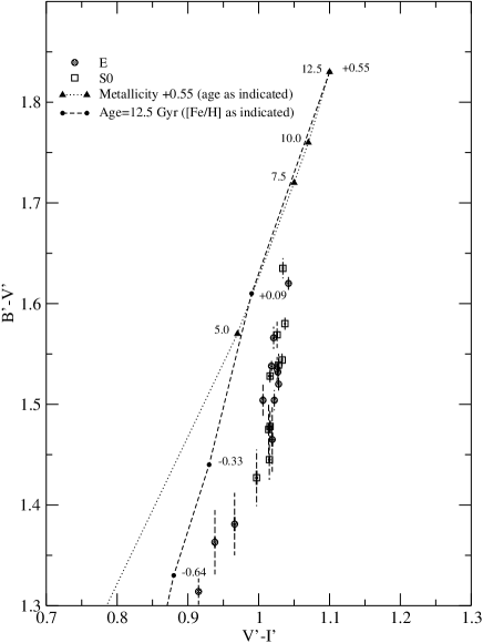
In order to model the stellar populations of the galaxies and derive gradients in age and/or metal abundance from the observed colour gradients, we need to determine the central colours as a boundary for the models. We plot these colours in a colour-colour diagram in Figure 2 (where the colour at $r=0$ is extrapolated from the linear fits), together with the predictions for a single-age stellar population with present age of 12.5 Gyr and metallicity varying between [Fe/H]=$+$0.55 and $-$2.5, and for a single-metallicity stellar population with metallicity of [Fe/H]=$+$0.55 and ages from 12.5 to 2.5 Gyr, as observed through the HST filters and at $z=0.18$. We used the latest version of the GALAXEV models of Bruzual & Charlot (2003) to realize these simulations adopting the Padova 1994 isochrones and Chabrier initial mass function, as recommended by Bruzual & Charlot (2003) and in the GALAXEV documentation.

One possible problem is that, as shown in Figure 2, the models are not fully capable of reproducing the central colours. This may be due to some small discrepancy in the population synthesis models, or to some inaccuracies in the extrapolation of central colours from the $r>0.3^{\prime\prime}$ data, or to the presence of dust in the galaxy cores (e.g. Peletier et al. 1999). However, the reddest (oldest and more metal rich) models are reasonably close to the actual values of the colours, especially in the $B^{\prime}-V^{\prime}$ colour which is most sensitive to stellar populations and most useful for our study, and we adopt this as the starting point for our modelling in interpreting the derived colour gradients.

Figure 2: Colour–colour plot for E (circles) and S0 (squares) galaxies and two BC2003 model lines, as identified in the legend. The values presented here are the central colours extrapolated from the fit to the data points presented in Figure 1. Solid error bars represent the statistical error while the dashed error bars show the systematic error.

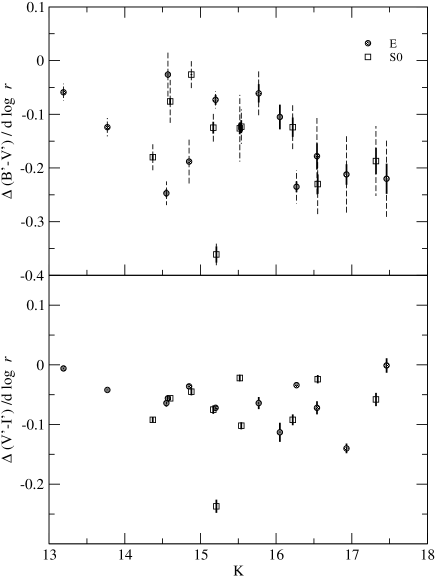
One of the aims of this paper is to investigate not only the evolution of the colour gradients at intermediate redshift and discuss them in the light of both local and higher redshift data (see below) but also to consider how the gradient size depends on galaxy luminosity and on morphology. We plot the derived colour gradients vs. $K$ magnitude (which is a good measure of the underlying stellar mass) in Figure 3. We use different symbols (circles and squares, as indicated in the caption) for E and S0 galaxies. We find little evidence that gradient size, in both colours, depends on either luminosity or morphology. The consequences of this finding are examined below.

Figure 3: Amplitude of the colour gradients in F450W$-$F606W (top panel) and F606W$-$F814W (bottom panel) as a function of $K$ magnitude. Symbols as in Fig. 2.

Naturally, our conclusions prevalently concern spheroids and the bulge components of S0 galaxies as our data, especially in $B^{\prime}$ where we are most sensitive to stellar populations, do not reach much into the disk dominated portion of the S0 galaxies. However, in some cases, Figure 1 shows that we are able to sample a small portion of the disk. This may be the case for # 280, 633, 205 and 137. It is apparent that the colours of these disks are at least qualitatively similar to those of their parent bulges, which would suggest that they have similar stellar populations. Fisher, Franx & Illingworth (1996) and Peletier & Balcells (1996) have also reached similar conclusions, although Fisher et al. (1996) also point out that the star formation histories may be different for at least some galaxies, despite their having similar ages.

Unfortunately, the small portions of the disks we survey are not sufficient to determine colour gradients for the disks and carry out a comparison with the bulge and therefore reconstruct the star formation and enrichment histories of the two components of the galaxies. This should be possible with more sensitive data from the ACS, some of which are available publicly and will be the subject of a later paper.

4 Discussion

We now examine the implications of our findings for models of galaxy formation and evolution: in particular, we consider simplistic models of formation by dissipational collapse and by hierarchical mergers as our benchmarks; these comparisons should probably be intended as a stimulus for more comprehensive modelling rather than setting true limits on the accuracy with which the models represent the observations

We first find that the size of the colour gradients is broadly independent of $K$ luminosity. Models of colour gradients in galaxies, unfortunately, do not yet reach this level of detail, but we naively expect that, in a monolithic collapse scenario, the size of the gradients will be proportional to the depth of the potential well, as the stellar population gradients are induced by superwinds, so that more massive galaxies have steeper colour gradients (Carlberg 1984). In general, monolithic collapse models yield excessively large gradients when compared to the observations (Carlberg 1984) but more detailed treatment of gas physics may alleviate this problem (e.g. Kawata 2001, Pipino & Matteucci 2004). In hierarchical merger models (White 1980, Kauffmann 1996, Cole et al. 2000) we expect that mergers will erase any colour gradients originally set up. Some gradients may be re-established by star formation at later epochs, but we might expect that more massive galaxies, at the top of the merging hierarchy, will experience more mergers and have flatter gradients. Our results appear to be inconsistent with either (admittedly simplistic) scenario, as we observe no evidence of strong trends in gradient size with luminosity.

Tamura & Ohta (2003) suggest that the brigher ($R<15$) and more massive galaxies in Abell 2199 show steeper gradients, which would be consistent with the predictions of monolithic collapse models, while La Barbera et al. (2004) favour no trend in the gradient size with luminosity, or possibly flatter gradients for brighter galaxies, in Abell 2163B, at $z\sim 0.2$ which is in somewhat better agreement with our observations and with hierarchical merger models. Study of the evolution of these trends with redshift may allow us to resolve this issue more decisively.

The observations suggest that there is no significant difference in the size of colour gradients between E and S0 galaxies bulges. This implies that the two systems have very similar distributions of stellar populations. We use our single stellar population models to calculate that the observed gradients are consistent with either a $\delta{\rm[Fe/H]}/\delta\log r\sim-0.3$ dex per decade gradient at a fixed 12.5 Gyr (present) age, or with an approximately 3 Gyr per decade age gradient at a fixed metallicity of [Fe/H]=+0.09, consistent with most previous work on this subject. The age–metallicity degeneracy, of course, prevents us from determining, from these data alone, which scenario is most likely.

We therefore follow previous work (Saglia et al. 2000, Tamura & Ohta 2000, La Barbera et al. 2003) in studying the evolution of colour gradients as a function of lookback time. Our $B^{\prime}$, $V^{\prime}$ and $I^{\prime}$ bands correspond approximately to the rest-frame $U$, $g$ and $R$ bands. Since few local studies are carried out in the $g$ band, we compare our results with observations in $U-V$ and $V-R$. Local values for $U-V$ and $V-R$ gradients for cluster galaxies are taken from the compilation of Idiart et al. (2002). We use the $U-V$ gradients for a $z=0.38$ cluster presented in Saglia et al. (2000); we have been unable to find $V-R$ data at higher redshift.

We plot these data and the mean values for colour gradients in A2218 in Figure 4, together with four models from La Barbera et al. (2003) that appear to be most appropriate to reproduce their observations. The parameters of these models are shown in Table 2, where the first column is the model ID and the subsequent columns represent the age at centre and outskirts, the metal abundance at centre and outskirts and the exponential decay time of the star formation. Here, model T1 has a central age of 13 Gyr and an outer age of 8 Gyr, with both stellar populations having a metallicity of $+0.09$: it corresponds to the model of the same name in La Barbera et al. (2003). Model Z1 has two stellar popularions of the same age (13 Gyr) but a metallicity gradient of 0.4 dex from center to edge. Model TZ has both a small age gradient (13 Gyr at the center and 11 at the edge) and a metal abundance gradient as in model T1. Finally, model T3 corresponds to La Barbera’s model $\sim T1$ (for spirals), has a small age gradient (2 Gyr from center to edge, with a central age of 13 Gyr) and metal abundance of $-0.33$ but $\tau$ of 3 Gyr, while all other models have $\tau$ of 1 Gyr (where $\tau$ is the exponential decay time for star formation). The actual values for the ages and metallicities of the models are slightly different from those used in La Barbera et al. (2003), as the cosmology and metallicity have changed in the latest GALAXEV models. We use the GALAXEV values that best approximate those used by La Barbera et al. (2003).

The models are unable to reproduce the central colours (Figure 2), which suggests that these galaxies may be more metal rich than [Fe/H]=$+0.55$ (this is likely due to the typical $\alpha$ element overabundances). Because of this, there is some doubt as to whether the derived gradients may be fairly compared to the observations. The actual values of the colour gradients from the models at $z=0.18$ are, for models T1,Z1,TZ and T3, respectively, $-0.40$, $-0.28$, $-0.35$ and $-0.19$ mag. in $U-V$ and $-0.08$, $-0.06$, $-0.08$ and $-0.05$ mag. in $V-R$. While all models are able to reproduce the $V-R$ gradients, they are a poor fit to the $U-V$ gradient, with the possible exception of model T3. However, if we consider the evolution of the gradients, model T3 predicts a gradient of $-0.13$ at $z=0$ and $-0.30$ at $z=0.38$, which compares badly with the measured values of $-0.17$ at $z=0$ (Idiart et al. 2002) and $-0.08$ at $z=0.38$ (Saglia et al. 2000). Since the models do not appear to reproduce the values of the gradients or the galaxy central colours, we choose to carry out a differential comparison by forcing the models in Figure 4 to run through the A2218 measurements.

Figure 4: Mean colour gradients in $B^{\prime}-V^{\prime}$ (top panel) and $V^{\prime}-I^{\prime}$ (bottom panel) for A2218 galaxies (circles for Es and squares for S0s; note the arbitrary offset from the cluster redshift introduced for purposes of clarity in presentation). Also plotted are literature values (Filled ‘up’ triangles: Idiart et al. 2002; filled ‘down’ triangles: Saglia et al. 2000) and four models whose parameters are described in Table 2 and in the text.

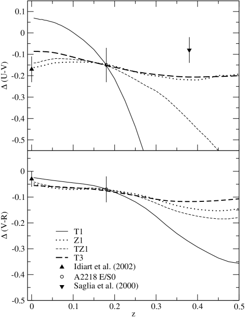
The main conclusion from this exercise is that the best model is the familiar small metallicity gradient (although a slightly smaller gradient may perform better), while a small age gradient model with large $\tau$ is marginally worse. Note that this latter model performs somewhat better in reproducing the actual values of the gradients. The combined age and metallicity model and the age gradient model are largely excluded by the data.

The similarity in the size of colour gradients for E and S0 galaxies suggests that their bulges, at least, have similar stellar populations and that these are also similarly distributed. The result confirms and extends the observations of Ziegler et al. (2001) and Mehlert et al. (2003) for bright S0 galaxies in Abell 2218 and the Coma cluster respectively: on the other hand, both Kunstchner & Davies (1998) and Mehlert et al. (2003) find that at least some S0s in Fornax and Coma, respectively, possess younger stellar populations, although these objects tend to be among the fainter S0s rather than the bright S0s. Similarly Smail et al. (2001) argue that the fainter S0s in their sample ($K>17$, or $L<0.1L^{*}$) may be more distinct from ellipticals. This need not be inconsistent with our findings, if bright S0s form in a different manner from the faint S0s: in particular, the evolution may take place mostly in the disks, while our results concern mostly bulges.

Our main conclusions are therefore that the observed trends in colour gradients are difficult to explain in the context of any of the popular models of galaxy formation, but stress the essential similarity of the stellar populations of bulge dominated systems. Observations of a larger sample of objects at higher resolution with ACS or WFPC3 should allow us to investigate these issues further. Investigations of colour gradients for S0 disks should allow us to achieve a better understanding of the relation between bulge and disk evolution, particularly with reference to the scenario in which spiral disks are converted to S0 disks via a variety of processes (ram stripping, truncation, starbursts induced by mergers or interactions, harassment, among others).

Table 2: Model parameters

Model	Age at centre	Age at outskirts	[Fe/H] at centre	[Fe/H] at outskirts	$\tau$
T1	13	8	$+$0.09	$+$0.09	1
Z1	13	13	$+$0.09	$-$0.33	1
TZ	13	11	$+$0.09	$-$0.33	1
T3	13	11	$-$0.33	$-$0.33	3

References

- (1)
- (2)
- Abraham et al. (1999) Abraham, R. G., Ellis, R. S., Fabian, A. C., Tanvir N. R., Glazebrook, K. 1999, MNRAS, 303, 641
- Baum et al. (1986) Baum, W. A., Thomsen, B. and Morgan, B. L. 1986, ApJ, 301, 83
- Bruzual and Charlot (2003) Bruzual A., G. and Charlot, S. 2003, MNRAS, 344, 1000
- Busko (1996) Busko, I. C. 1996, Astronomical Data Analysis Software and System V, ASP Conference Series 101, G. H. Jacoby and J. Barnes, p. 139
- Butcher and Oemler (1984) Butcher, H. and Oemler, A. 1984, ApJ, 285, 426
- Carlberg (1984) Carlberg, R. 1984, ApJ, 286, 403
- Carollo et al. (1993) Carollo C. M., Danziger, I. J. and Buson, L. 1993, MNRAS, 265, 553
- Cole et al. (2000) Cole S., Lacey C. G., Baugh C. M., Frenk C. S. 2000, MNRAS, 319, 168
- Davies et al. (1993) Davies, R. L., Sadler, E. M. and Peletier, R. F. 1993, MNRAS, 262, 650
- Dressler (1980) Dressler, A. 1980, ApJ, 236, 351
- Fisher et al. (1996) Fisher D., Franx M. and Illingworth, G. D. 1995, ApJ, 459, 110
- Franx et al. (1989) Franx, M., Illingworth, G. and Heckman, T. 1989, AJ, 98, 538
- Goudfrooij et al. (1994) Goudfrooij, P., Hansen, L., Jørgensen, H. E., Nørgaard-Nielsen, H. U., de Jong, T. and van den Hook, L. B. 1994, A&AS, 104, 179
- Hubble (1936) Hubble E. P. 1936, The Realm of the Nebulae, Yale University Press
- Hinkley and Im (2001) Hinkley, S. and Im, M. 2001, ApJ, 560, L41
- Holtzman et al. (1995) Holtzman, J. A., Burrows, C. J., Casertano, S., Hester, J., Trauger, J. T., Watson, A. M. and Worthey, G. 1995, PASP, 107, 1065
- Idiart et al. (2002) Idiart, T. P., Michard, R. and de Freitas Pacheco, J. A. 2002, A&A, 383, 30
- Jedrzejewski (1987) Jedrzejewski, R. L. 1987, MNRAS, 226, 747
- Kauffmann (1996) Kauffmann G. 1996, MNRAS, 281, 487
- Kawata (2001) Kawata, D. 2001, ApJ, 558, 598
- Kormendy and Bender (1996) Kormendy J. and Bender R. 1996, ApJ, 464, L119
- Kunstchner and Davies (1998) Kunstchner H. and Davies R. L. 1998, MNRAS, 295, 43
- La Barbera et al. (2003) La Barbera, F., Busarello, G., Massarotti, M., Merluzzi, P. and Mercurio, A. 2003, A&A, 409, 21
- La Barbera et al. (2004) La Barbera, F., Merluzzi P., Busarello, G., Massarotti, M. and Mercurio, A. 2004, A&A, 425, 797
- Larson et al. (1980) Larson, R. B., Tinsley, B. M. and Caldwell, C. N. 1980, ApJ, 237, 692
- Mehlert et al. (2003) Mehlert, D., Thomas, D., Saglia, R. P., Bender, R., Wegner, G. 2003, A&A, 407, 423
- Micol et al. (1997) Micol A., Bristow P., Pirenne B. 1997, in The 1997 HST Calibration Workshop with a new generation of instruments ed. S. Casertano, R. Jedrzejewski, C. D. Keyes and M. Stevens (Baltimore: Space Telescope Science Institute)
- Michard (1994) Michard R. 1994, A&A, 288, 401
- Peletier et al. (1990) Peletier, R. F., Davies, R. L., Illingworth, G. D., Davis, L. E. and Cawson, M. 1990, AJ, 100, 1091
- Peletier and Balcells (1996) Peletier R. and Balcells M. 1996, AJ, 111, 2238
- Peletier et al. (1999) Peletier, R. F., Balcells, M., Davies, R. L., Andredakis Y., Vazdekis, A., Burkert, A. and Prada, F. 1999, MNRAS, 310, 703
- Pimbblet (2003) Pimbblet K. A. 2003, PASA, 20, 294
- Pipino and Matteucci (2004) Pipino, A. and Matteucci, F. 2004, MNRAS, 347, 968
- Saglia et al. (2000) Saglia, R., Maraston, C., Greggio, L., Bender, R. and Ziegler, B. 2000, A&A, 360, 911
- Smail et al. (2001) Smail, I., Kuntschner, H., Kodama, T., Smith, G. P., Packam, C., Fruchter, A. S., Hook, R. N. 2001, MNRAS, 323, 839
- Tamura et al. (2000) Tamura, N., Kobayashi, C., Arimoto, N., Kodama, T. and Ohta, K. 2000, AJ, 119, 2134
- Tamura and Ohta (2002) Tamura, N. and Ohta, K. 2000, AJ, 120, 533
- Tamura and Ohta (2003) Tamura, N. and Ohta, K. 2003, AJ, 126, 596
- White (1980) White, S. D. M. 1980, MNRAS, 191, 1
- Worthey (1996) Worthey, G. 1996, in New light on galaxy evolution, IAU Symposium 171, ed. R. Bender and R. L. Davies (Dordrecht: Kluwer), p. 71
- Ziegler et al. (2001) Ziegler, B., Bower, R. G., Smail, I., Davies, R. L., Lee, D. 2001, MNRAS, 325, 1571