Optically Identified BL Lacertae Objects from the Sloan Digital Sky Survey

Abstract

We present a sample of 386 BL Lacertae (BL Lac) candidates identified from 2860 deg² of the Sloan Digital Sky Survey (SDSS) spectroscopic database. The candidates are primarily selected to have quasi-featureless optical spectra and low proper motions as measured from SDSS and USNO-B positions; however, our ability to separate Galactic from extragalactic quasi-featureless objects (QFOs) on the basis of proper motion alone is limited by the lack of reliable proper motion measurements for faint objects. Fortunately, high proper motion QFOs, mostly DC white dwarfs, populate a well defined region of color space, approximately corresponding to blackbodies with temperatures in the range 7000–12000 K. QFOs with measurable redshifts or X-ray or radio counterparts (i.e., evidence of an extragalactic/AGN nature) loosely follow a track in color space that corresponds to power-law continua plus host galaxy starlight, with typical power-law slopes in the range $1<\alpha_{\mathrm{opt}}<2$ ($f_{\nu}\propto\nu^{-\alpha}$). Based largely on this remarkably clean color separation, we subdivide the sample into 240 probable candidates and 146 additional less probable (likely stellar) candidates. The probable BL Lac candidates have multi-wavelength properties consistent with the range of previously known BL Lacs, with an apparent preponderance of objects with synchrotron peaks at relatively high energies (HBL/XBL-type). The majority of the 154 objects with measurable redshifts have z $<1$, with a median of 0.45; there are also a handful of high-redshift objects extending up to z $=5.03$. We identify a small number of potential radio-quiet BL Lac candidates, although more sensitive radio observations are needed to confirm their radio-quiet nature.

1 Introduction

Among the rarest and most extreme of the various observational classes of Active Galactic Nuclei (AGN) are the BL Lacertae objects (BL Lacs). The defining traits of BL Lacs generally include: a broad, rapidly variable, non-thermal spectral energy distribution (SED) with significant power from radio wavelengths to X-rays and $\gamma$-rays; lack of the strong optical emission lines that typify other AGN; high and variable polarization at optical and radio wavelengths; and compact, core-dominated radio morphology (Kollgaard, 1994). All of the above properties can be reproduced naturally by a model in which the dominant source of the observed emission is a relativistic jet of plasma directed within a small angle to the line of sight (e.g., Blandford & Rees 1978). This picture is particularly appealing because there is a known class of objects that plausibly consists of physically identical systems in which the jet is directed at a more substantial angle to the line of sight, namely the Fanaroff-Riley class I (FRI; low-power; Fanaroff & Riley 1974) radio galaxies. The beamed counterparts of more powerful FRII radio galaxies are generally believed to be flat-spectrum radio quasars (FSRQs), although FSRQs have emission line properties more like those of typical broad-line AGN. BL Lacs (at lower typical luminosity) and FSRQs (at higher luminosity) are often grouped together under the designation of blazars. This scenario is favored in unification schemes for radio-loud AGN (Urry & Padovani, 1995).

Traditionally, BL Lacs have been discovered from observations at either radio (e.g., Stickel et al. 1991) or X-ray (e.g., Stocke et al. 1991; Schachter et al. 1993; Perlman et al. 1996) frequencies. Such radio and X-ray selected samples of BL Lacs are known to be composed of objects with systematically different properties, such as the peak frequencies of the spectral energy distributions (SEDs), as discussed by Padovani & Giommi (1995). Those authors coined the terms ‘low-energy cutoff BL Lacs’ (LBLs) and ‘high-energy cutoff BL Lacs’ (HBLs) to distinguish the types of objects predominantly found in radio and X-ray selected samples, respectively; the obvious acronyms RBL and XBL are often used to make the same distinction. It has been proposed that blazar properties follow a continuous sequence from BL Lacs into the regime of FSRQs; in this scenario an object’s observed characteristics are determined by the angle between the jet axis and the line of sight, the overall jet power, and possibly another parameter (Fossati et al., 1998; Ghisellini et al., 1998).

Large optical surveys, such as the Sloan Digital Sky Survey (SDSS; York et al. 2000) and the Two-degree Field QSO Redshift Survey (2QZ; Boyle et al. 2000), have the potential to reveal new populations of BL Lacs with different properties from the well known radio or X-ray selected objects. Londish et al. (2002) presented a sample of several dozen objects from the 2QZ selected on the basis of having quasi-featureless optical spectra resembling those of BL Lacs; however, some of these objects were found to be significantly fainter in the radio, relative to the optical, than classical BL Lacs. At least one of these latter objects has been confirmed to be extragalactic via a redshift measurement obtained in a follow-up observation (Londish et al., 2004); along with a small number from other searches (Fan et al., 1999; Anderson et al., 2001), these objects are potential radio-quiet BL Lacs or weak-lined radio-quiet quasars. Whether or how such objects fit into the blazar sequence or more generally into the AGN unification picture are open questions.

In the present work, we describe a sample of 386 optically-identified BL Lac candidates compiled from 2860 deg² of the SDSS spectroscopic survey. As in Londish et al. (2002), these objects are selected to have quasi-featureless optical spectra and are identified solely on the basis of their optical properties and lack of significant proper motions. We discuss the degree to which the sample remains contaminated by featureless stars, either lacking reliable proper motion measurements, or simply having proper motions below the detection threshold. We subdivide the sample into 240 “probable” and 146 “possible” candidates based on all available information. We search the sample for exceptional objects, such as radio-quiet BL Lacs (or lineless radio-quiet quasars), and we explore how our sample fits into the overall understanding of the blazar class. Our probable BL Lac candidates are not a complete sample, but are more numerous than any previous sample of BL Lacs of which we are aware, and represent a significant addition to the $\sim 400$ previously known BL Lacs.

In §2 we describe the SDSS observations and data processing. In §3 we discuss the selection of quasi-featureless spectra and the use of proper motion to reject weak-featured stellar objects. In §4 we cross-correlate our sample with the ROSAT All-Sky Survey (RASS) X-ray source catalogs and with the Faint Images of the Radio Sky at Twenty cm (FIRST) and NRAO/VLA Sky Survey (NVSS) radio catalogs. In §5 we analyze the redshift distribution, optical colors, and multi-wavelength properties of our BL Lac candidates. In §6 we lay out some prospects for follow-up studies, and in §7 we summarize our primary results.

2 SDSS observations and data pipeline

The Sloan Digital Sky Survey is a multi-institutional effort to obtain high-quality 5-band (SDSS $ugriz$; Fukugita et al. 1996; Hogg et al. 2001; Smith et al. 2002) photometric imaging of a large fraction ($\approx 10000$ deg²) of the sky, principally the northern Galactic cap and a stripe along the celestial equator, with spectroscopic follow-up of interesting samples of objects, primarily galaxies ($\sim 10^{6}$) and quasars ($\sim 10^{5}$). The SDSS uses a dedicated 2.5 m telescope at Apache Point Observatory with a $2.5^{\circ}$ 30-CCD mosaic camera (Gunn et al., 1998) and two multi-object spectrographs with 320 $3^{\prime\prime}$ fibers each (e.g., Stoughton et al. 2002). Imaging data are processed through automated software pipelines (Lupton et al., 2001; Pier et al., 2003), in which the data are photometrically and astrometrically calibrated and objects are detected, measured, and classified. The photometric calibration is typically better than 2% (Ivezić et al., 2004), and the astrometric calibration is better than $0\farcs 1$ root-mean-square (rms) per coordinate.

2.1 Targeting for spectroscopy

Once a region of sky has been imaged, subsets of the objects detected are then selected for spectroscopic observations on the basis of their photometric and other properties. Resolved objects are targeted to $r=17.77$ for the main galaxy sample (Strauss et al., 2002), and luminous red galaxies are targeted based on their colors to $r=19.5$ (Eisenstein et al., 2001). Quasar candidates are targeted as outliers from the stellar locus or as point-like FIRST sources to $i=19.1$ for the low-redshift sample; objects very red in $u-g$, $g-r$ or $r-i$ (and having colors consistent with Ly$\alpha$ absorption cutting into the observed frame optical flux) are targeted to $i=20.2$ for the high-redshift quasar sample (Richards et al., 2002). Ultraviolet-excess (UVX; dereddened $u-g<0.6$) objects with non-stellar colors are explicitly included in the low-redshift sample. Objects can also be targeted by a variety of serendipity algorithms to $g=20.5$ or $i=20.5$. These selection routines cover regions of color space outside the main stellar locus but not included by quasar target selection; they also include objects with radio counterparts detected by the FIRST survey (Becker et al., 1995; Ivezić et al., 2002) or X-ray counterparts from the ROSAT All Sky Survey (RASS; Voges et al. 1999; Anderson et al. 2003). Spectroscopic fibers are allocated by a tiling algorithm (Blanton et al., 2003), which gives top priority to the main quasar and galaxy samples (along with fibers needed for calibration purposes).

2.2 Processing of spectra

Raw spectral data are reduced and calibrated (e.g., Stoughton et al. 2002), and individual spectra, which cover the wavelength range 3800–9200 Å with an approximate resolution of $\lambda/\Delta\lambda\approx 1800$, are then automatically processed to classify them (star, galaxy, or quasar) and determine redshifts.

In our analysis, we use the output of the classification/redshift-finding routine “SpecBS” (written by D. Schlegel). This algorithm classifies spectra by performing separate $\chi^{2}$-fits to the spectra using linear combinations of different models — sets of galaxy or quasar eigenspectra or stellar templates — plus 2nd or 3rd order polynomials, with redshift/radial velocity as a free parameter. An object is classified as a star, galaxy or quasar, according to which type of model produces the best $\chi^{2}$ value. Redshift warning flags are set if there are multiple models that provide nearly equivalent $\chi^{2}$ values or if other problems are present, such as limited wavelength coverage due to lost data, unreasonable behavior like negative templates, or large numbers of statistically anomalous data points.

The polynomial component, which may be positive or negative, is included to account for (generally low-level) variations of individual objects from the templates and to compensate for contamination (e.g., star-galaxy blends) or flux-calibration problems (cf. discussion in Abazajian et al. 2004), as well as to assist in fitting the spectra of unusual (e.g., heavily reddened) objects. Objects with the quasi-featureless spectra we seek will generally require strong polynomial components in order to achieve adequate fits, as discussed in the next section. In the most extreme cases, the polynomial components can completely dominate the fits; for such objects the spectral classifications and redshifts are clearly meaningless.

3 Sample selection

In order to avoid the selection biases that enter into the construction of radio and X-ray-selected samples of BL Lacs to the greatest degree possible, we confine our selection criteria strictly to the optical properties of objects in the SDSS spectroscopic database. Of course, objects enter into that data set via a variety of target selection algorithms as described in the previous section, some of which are based on X-ray or radio emission. However, by keeping track of the reasons for which each object was targeted for spectroscopy, we can account after the fact for selection biases introduced by these factors (see discussion in §5.5).

Most of the sky coverage of SDSS is imaged in one epoch only. Spectroscopic observations of a given field typically lag behind imaging by anywhere from approximately one month to one year. A detailed study of the variability of spectroscopically-confirmed quasars using the photometric+spectroscopic observations is presented by Vanden Berk et al. (2004a). For our purposes however, (usually) having only two epochs of observation in total for a given spectroscopic object precludes complete selection on the basis of variability. Another optical property that could be used to identify BL Lacs would be polarization (e.g., Jannuzi et al. 1993), but this is not among the capabilities of the SDSS.

Therefore, the spectroscopic phase of our BL Lac candidate selection is primarily based on a single property: lack of strong features (i.e., emission or absorption lines) in the optical spectra. While this approach is clearly biased toward objects that are dominated by the continuous emission from the jet at optical wavelengths (and subject to the effects of SDSS spectroscopic target selection), this bias should differ from those that affect classical radio or X-ray selected samples and therefore may be sensitive to new populations of BL Lacs missed by previous surveys. This is the same approach used by Londish et al. (2002).

The parent sample for our search is the SDSS spectroscopic database as of mid-July 2002, comprising over 345,000 individual spectra and covering about 2860 square degrees of sky [roughly the area covered by Data Release Two (DR2); Abazajian et al. 2004]. The initial selection was performed using a somewhat older version of the spectroscopic data reduction pipeline, approximately corresponding to Data Release One (DR1; Abazajian et al. 2003). In that version there were (known) spectrophotometric problems, especially in the 3800-4400 Å range, such as artificial structure resembling emission or absorption features; we employed caution in our search so as not to mistake these and other data reduction artifacts for real spectral structure. These problems have been corrected to a large degree in DR2 and later reductions (cf. Abazajian et al. 2004). As previously stated, we use the SpecBS spectroscopic classifications and spectral fits (contemporaneous with DR2); all other data presented in this paper (e.g., photometry, astrometry, etc.) are from the official DR2 reductions, unless stated to the contrary.

3.1 Selection of quasi-featureless spectra

The goal of our search is to extract all high-quality SDSS spectra that are consistent with the featureless or quasi-featureless spectrum of a BL Lac object, without regard to the continuum slope. Depending on intrinsic luminosity, redshift, and the details of AGN physics, these objects may show (a) host galaxy signatures such as stellar absorption features (e.g., Ca II H&K) or emission lines from associated H II regions (in which case there is a good chance that the image of the object will also show spatially resolved structure), (b) weak broad or narrow emission lines associated with AGN activity, (c) metal absorption lines or Ly$\alpha$ forest absorption from intervening material along the line of sight, or (d) no features whatsoever, to the limit of the SDSS spectral sensitivity (typically better than a few Å equivalent width for narrow features, for the objects that satisfy our signal-to-noise criteria; see §3.1.1). Especially for the truly featureless objects, we reiterate that the spectral classifications and redshifts obtained from the spectroscopic pipeline will be meaningless.

A complication inherent in this approach is that BL Lacs are not the only type of objects known to have featureless optical spectra. In particular, white dwarfs (WDs) of class DC share this property (e.g., Wesemael et al. 1993; Londish et al. 2002). This is not an issue for objects that fall into classes (a)–(c) above. To distinguish true BL Lacs of class (d) from DC WDs without resorting to multi-wavelength properties, the best available test is to use proper motion (see §3.2 below). In what follows, we shall refer to objects that satisfy our spectral selection criteria as quasi-featureless objects (QFOs); we shall reserve the term “BL Lac candidate” for objects that satisfy the additional proper motion requirement described in §3.2.

3.1.1 Signal-to-noise requirement

In order to restrict our analysis to objects for which reliable spectral classifications are possible, we first impose a signal-to-noise ratio ($S/N$) requirement. We analyze the spectral flux density (erg cm^-2 s^-1 Å^-1) in three 500 Å-wide regions centered at 4750, 6250, and 7750 Å in the observed frame; these are chosen to be regions in which we find SDSS spectra to be of generally high quality, with minimal sky contamination and calibration problems, and which fall within the $g$, $r$ and $i$ filters respectively. We define the signal $S$ in each of these regions to be $S=\sum_{i}(f_{\lambda,i}/\sigma_{i}^{2})/\sum_{i}(1/\sigma_{i}^{2})$, where $f_{\lambda,i}$ and $\sigma_{i}$ are the flux density and estimated uncertainty in spectral element $i$. The error $N$ on this quantity is simply $N=[\sum_{i}1/\sigma_{i}^{2}]^{-1/2}$; therefore the signal-to-noise ratio for each region is $S/N=(\sum_{i}f_{\lambda,i}/\sigma_{i}^{2})/(\sum_{i}1/\sigma_{i}^{2})^{1/2}$. We keep only objects for which $S/N>100$ in one or more of these spectral regions. This corresponds to fiber magnitudes of roughly $g<20.5$, $r<20.3$ or $i<19.6$ for a typical spectroscopic plate.

3.1.2 Objects classified as stars or galaxies

Stars and galaxies together account for the majority (89%) of all SDSS spectroscopic objects. Most of these are well fit by stellar templates or combinations of galaxy eigenspectra, respectively, without the need for significant polynomial components in the fits (see §2.2). This is true only for objects which have characteristic stellar or galactic spectral energy distributions (SEDs) and absorption features of typical strength; such objects clearly do not qualify as quasi-featureless. In order to separate such objects from potential QFOs, we examine the relative importance of the polynomial component in the fit in two spectral regions: 3800–4200 Å and 8800–9200 Å (in the observed frame; near the blue and red ends respectively of the SDSS spectral coverage). We define the ratio $R\equiv P/S$, where $P$ is the average value of the polynomial in a region and $S$ is the spectral signal as defined in the previous subsection. If $S/N<25$ in both regions, the values of $R$ are not very meaningful and the test cannot be applied; such objects are rejected from further consideration. (This is similar to the $S/N$ requirement described in the previous subsection but much less stringent.) We reject objects classified by SpecBS as stars or galaxies for which $R_{\mathrm{blue}}<0.6$ and $R_{\mathrm{red}}<0.5$; the blue cutoff is more stringent due to the large number of absorption features in this wavelength region for many stellar types and the presence of the Ca II H&K break in galaxy spectra. This step eliminates approximately 80% of stars and 96% of galaxies.

We do not reject objects classified as quasars based on the values of $R$. Due to the range of quasar emission line strengths and the power-law nature of quasar continuum emission, some quasi-featureless objects may be well fit by combinations of quasar eigenspectra (through the observed wavelength range) without the need for a strong polynomial component.

Objects classified as stars that survive the previous cut are then subjected to a test for absorption features appropriate to the SpecBS-fit stellar type. We test stars classified as O, B, or A for absorption lines from He II, He I, and the H-Balmer series. We test F and G stars for the H-Balmer series and lines from Ca II, Mg I, and Na I. We test K stars for Ca I, Ca II, Mg I, and Na I lines. We test M stars for Ca II and Na I lines and TiO molecular absorption bands. We measure the significance of all absorption features by comparing the spectral flux in pre-defined continuum regions on either side of the absorption to the spectral flux within the absorption feature. Objects are rejected if two or more absorption features are detected with $\geq 3\sigma$ significance; we require the detection of at least two features to decrease the chance of inadvertently rejecting extragalactic objects showing absorption lines from intervening material. Examples of objects with weak stellar features or featureless spectra are displayed in Figure 1.

We test objects classified as galaxies for the strength of the Ca II H&K break (at the pipeline redshift) if it is present in the spectra and if no redshift warning flags have been set. The Ca II H&K break strength is defined as

$$C=0.14+0.86(f_{\lambda,+}-f_{\lambda,-})/f_{\lambda,+},$$ (1)

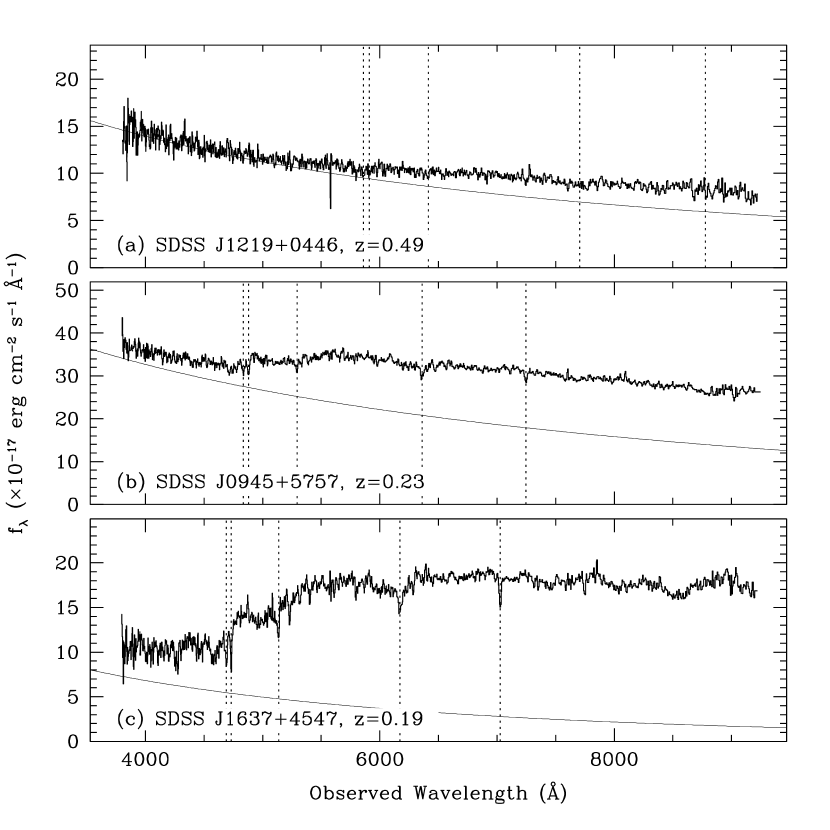
Figure 2: Example SDSS spectra of QFOs with noticeable host galaxy features of varying strengths and secure redshift measurements. The format is the same as Figure 1. The dotted lines mark the positions of stellar absorption lines at the appropriate redshifts. Objects (a) and (b) are unambiguous BL Lac candidates. Object (c) represents a marginal case for a BL Lac: it has a Ca II H&K break strength of 0.36, larger than the classical cutoff of 0.25 but within our acceptable range of $<0.4$. All three objects enter the sample of QFOs.

where $f_{\lambda,-}$ and $f_{\lambda,+}$ are the average flux densities in the rest-frame wavelength regions 3750–3950 Å and 4050–4250 Å respectively (e.g., Landt et al. 2002). (The form of this equation derives from the fact that it is historically measured in $f_{\nu}$ as in Bruzual 1983, rather than $f_{\lambda}$.) We reject objects for which $C>0.4$ (as in Marchã et al. 1996) and $|C/\delta C|>3$ where $\delta C$ is the uncertainty on $C$. Stocke et al. (1991) adopted a more conservative cut of 0.25, but we err on the liberal side in order not to reject any intrinsically red BL Lacs with significant host galaxy contamination. Several examples of objects with a range of host galaxy contributions that survive the polynomial and Ca II H&K cuts are given in Figure 2.

3.1.3 Objects classified as quasars and other emission line objects

For all objects classified as quasars, and for objects classified as stars or galaxies that survive the cuts described in the previous subsection, we test for the presence of emission lines at the pipeline redshift. We measure the equivalent width (EW) of an emission line by comparing the integrated flux in a pre-defined wavelength region around the center of the line with a linear approximation to the continuum in that region of the spectrum. The continuum level is determined by examining the flux in pre-defined regions on either side of the line. Special care is taken to examine potential continuum regions for the presence of absorption lines (e.g., metal lines from intervening material), which could artificially lower the continuum level and thereby exaggerate EW measurements. We do not attempt to automatically measure the EW of the Ly$\alpha$ emission line due to the frequently-complex absorption toward shorter wavelengths. This is to protect against inadvertently rejecting any BL Lacs at high enough redshift to show absorption from the Ly$\alpha$ forest (e.g., Fan et al. 1999).

We reject all objects in which any identified emission line has a rest-frame equivalent width (RFEW) greater than 5 Å at 1-$\sigma$ (i.e., the 1-$\sigma$ error on RFEW does not overlap 5 Å). This criterion is in accordance with the classical definition of a BL Lac, but is rather strict by modern standards (e.g., Marchã et al. 1996) in that it may cause us to reject objects with featureless AGN continua plus emission lines from host-galaxy star formation. However, we employ it in order not to be overwhelmed by galaxies with moderate star formation rates, which exist in the SDSS spectroscopic data in large numbers.

A line identification is considered secure only if other spectral features are present at the same redshift; thus a line identification implies that a redshift can be determined. If a single emission feature appears to be present but a line identification cannot be unambiguously determined, we do not reject the object. These criteria are designed so that quasi-featureless objects (possibly having bumpy spectra, e.g., due to intervening absorption) will not be rejected no matter what redshift the pipeline assigns them. Example spectra of borderline emission-line objects are shown in Figure 3.

3.1.4 Manual examination and frequent contaminants

The selection procedure described above is performed by an automated algorithm; however, the algorithm is designed to err on the side of caution so as not to inadvertently reject unusual and interesting objects. The result is that 3527 spectra (1.02% of the parent sample) survive through the automated stage and must be manually examined. At this stage we stringently reject remaining emission-line objects for which unambiguous line identifications can be made (with $RFEW>5$Å), objects with visibly-identifiable stellar features near zero redshift, and objects with data reduction problems or various forms of contamination (e.g., star-galaxy blends). All objects in Figures 1–3 survived until at least the manual selection stage due to the conservative design of the automated algorithm.

In addition to the quasi-featureless objects we seek, several distinct types of objects survive in significant quantities until the manual examination stage. Among these are quasars with relatively weak emission lines such as the object shown in panel (b) of Figure 3. Broad absorption line (BAL) quasars (e.g., Hall et al. 2002; Reichard et al. 2003) also survive in large numbers. Their frequently complicated spectra render it difficult to define continuum regions for measuring emission line EWs; we reject objects in which BAL troughs prohibit emission line measurements. Another class of frequent contaminants are blue, low-surface brightness galaxies. The spectra of these objects often show weak or washed-out absorption features; however, they are easily identified by their image properties. A final type of frequent contaminant are white dwarfs with weak-to-undetectable absorption features; many of these objects survive through the manual examination step and are discussed in the following subsection. Among weak-featured WDs several types stand out, including weak DQ (carbon) WDs (e.g., Liebert et al. 2003) and weak DB (helium) WDs. Kleinman et al. (2004) present a catalog of WDs from SDSS, including many with very weak spectral features or apparently featureless spectra.

3.2 Removing contamination by weak-featured white dwarfs

After the final examination of all remaining spectra, we are left with a sample of 580 quasi-featureless objects out of the original $\approx 345,000$. Of these, many are expected to be DC white dwarfs, which also fulfill the requirement of having featureless optical spectra. (A total of 124 of the 580 QFOs appear in the Kleinman et al. 2004 catalog; cf. §3.2.3 and 5.3.) Additionally there may be other weak-lined stellar objects and possibly extragalactic non-BL Lac QFOs (e.g., Fan et al. 1999; Londish et al. 2004), which would be of great interest.

In order to separate Galactic from extragalactic objects, several tests can be performed. One is the determination of a redshift/radial velocity based on spectral features. A second property that can indicate an extragalactic nature is image morphology: well-resolved objects (as reported by the photometric pipeline) in SDSS are mostly galaxies. However, these tests are redundant in many cases, since QFOs in which the host galaxy component is strong enough to be detected in the image also generally show noticeable host galaxy features in the spectra. Furthermore, these tests work most poorly for the most featureless objects.

A superior test is a measurement of proper motion, as in Londish et al. (2002). Galactic objects may have measurable proper motions, depending on kinematic properties, distance from the observer, astrometric precision and time baseline. Since DC WDs have low luminosities, those that are bright enough for SDSS spectroscopy should be relatively nearby, within a few hundred pc. For reference, a transverse velocity of 20 km s^-1 at a distance of 200 pc corresponds to a proper motion of 21 mas yr^-1. On the other hand the proper motions of extragalactic objects such as BL Lacs should be consistent with zero.

As of DR2, proper motions for SDSS objects are determined by matching with the United States Naval Observatory-B1.0 catalog (USNO-B; Monet et al. 2003). In the area covered by the SDSS, the USNO-B catalog is mainly derived from POSS-I and POSS-II plates, with time baselines in the range 20–51 yr. More accurate proper motions can be realized by using SDSS positions to recalibrate USNO-B astrometry; the maximum time baselines (POSS-I to SDSS) lie in the range 33–53 yr for objects discussed in this paper. This approach has been implemented by Munn et al. (2004) and Gould & Kollmeier (2004). We use the Munn et al. (2004) catalog, extended to include SDSS objects beyond DR1; all but four of the 580 QFOs appear in the extended catalog at the time of writing.

3.2.1 Proper motion assessment

Some SDSS objects do not have counterparts in USNO-B due to the difference in sensitivity and other factors, and mismatches occur in the proper motion catalog for this and other reasons. Therefore it is necessary to evaluate, based on available information, whether an individual proper motion measurement is or is not reliable. We consider proper motions only for objects that are spatially unresolved in the SDSS images; the Munn et al. (2004) approach uses galaxies (resolved objects) to recalibrate USNO-B astrometry, and thus the proper motions of resolved objects are (almost always) consistent with zero by construction. We adopt the following set of reliability criteria: (1) we require a one-to-one match between SDSS and USNO-B; (2) we require that the object be detected on at least four of the five USNO-B plates, including both POSS-I plates; (3) we require that the rms residuals for the proper motion fit be less than 525 mas yr^-1 in both right ascension and declination; (4) we require that there be no neighbor with $g<22$ within 7 arcsec. Requirements (1) and (2) ensure that the match between SDSS and USNO-B is likely to be correct. A larger residual than required in (3) indicates that the fit to the proper motion was poor, in that at least one detection lay well off a linear fit; 525 mas yr^-1 is an empirical cut (more lenient than that employed by Munn et al. 2004, but the same as used by Kilic et al. 2005) that includes the full distribution of residuals seen for good fits. Requirement (4) is designed to avoid errors introduced by blending on the Schmidt plates that make up the USNO-B catalog and is discussed in detail by Kilic et al. (2005). According to these criteria, 334 out of 580 QFOs have reliably measured proper motions.

In order to confirm the utility of these “reliable” proper motions to distinguish between Galactic and extragalactic objects, we compiled a sample of 3202 spectroscopically confirmed SDSS quasars with secure redshifts (and therefore no doubt as to their extragalactic nature). Of these, 2092 have reliably measured proper motions. Figure 4 shows the distribution of reliable quasar proper motions; 1987/2092$=$95.0% have measured proper motions $\mu<11$ mas yr^-1. This is almost identical to the Munn et al. (2004) result despite the use of somewhat different reliability criteria. Figure 5 shows reliable proper motions as a function of $r$-band magnitude for comparison quasars and QFOs. It is evident that a proper motion cut of 11 mas yr^-1 effectively separates out a large number of QFOs with unambiguously significant proper motions, even toward the faint end. Therefore, in what follows we shall consider proper motions $\mu\geq 11$ mas yr^-1 to be significant, and proper motions $\mu<11$ mas yr^-1 to be insignificant, unless otherwise stated.

3.2.2 Proper motions and optical colors

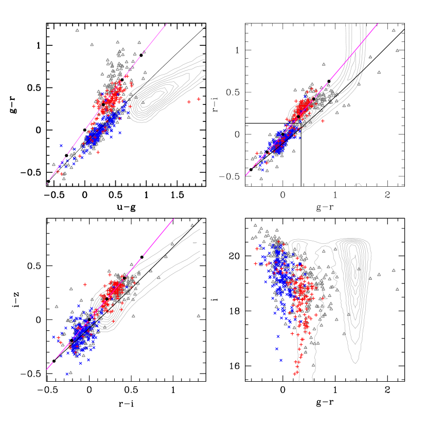
Figure 6: Color-color and color-magnitude diagrams of SDSS quasi-featureless objects; no correction for Galactic reddening has been applied. Contours represent the stellar locus (e.g., Finlator et al. 2000). Diagonal magenta lines in the color-color diagrams show the loci of objects with pure power-law spectra, black dots on these lines correspond to $\alpha=-2,-1,0,1,2,3$ ($f_{\nu}\propto\nu^{-\alpha}$) from lower left to upper right, and diagonal black lines show the loci of blackbody colors. Red ‘+’ signs show objects with reliably measured proper motions $\mu<11$ mas yr^-1; blue ‘$\times$’ marks are those with reliable proper motions $\mu\geq 11$ mas yr^-1; grey triangles are objects that lack reliable proper motion measurements. The apparent correlation between $g-r$ color and $i$ magnitude is due to a combination of SDSS target selection and $S/N$ selection effects, as discussed in §3.2. The solid-outline box in the upper right panel is the “blue-$gri$” region.

Figure 6 shows SDSS color-color and color-magnitude diagrams for quasi-featureless objects, symbolically divided according to proper motion at 11 mas yr^-1. We have not corrected for the Galactic extinction/reddening, since many of the QFOs are expected to be DC WDs; these objects have low luminosities (absolute magnitudes $M_{\mathrm{B}}\sim 14$; McCook & Sion 1999), and thus should be relatively nearby and may not be significantly reddened. [In Figure 6 and elsewhere, we use point-spread function (PSF) magnitudes.]

In addition to a handful of QFOs scattered around in color space, two populations of QFOs are evident in Figure 6. The objects with significant proper motions are, as a group, blue in $g-r$, $r-i$ and $i-z$, and have colors that approximately follow the blackbody color locus for temperatures in the range 7000–12000 K. There is also a large group of objects without significant proper motions that approximately follow the power-law color locus and extend toward the red; these objects are mostly concentrated in the range $1<\alpha_{\mathrm{opt}}<2$. (We define all slope parameters $\alpha$ in the sense $f_{\nu}\propto\nu^{-\alpha}$.) These two groups of objects are remarkably distinct from one another. The region defined by ($g-r<0.35$; $r-i<0.13$) — the “blue-$gri$” region — as delineated in the upper right panel of Figure 6, contains the vast majority (191/197) of objects with significant proper motions, while it contains only 23/137 of the objects without significant proper motions.

It is plausible that the 23 blue-$gri$ QFOs with reliable proper motions $\mu<11$ mas yr^-1 simply represent the low-proper-motion extension of the population of QFOs with significant proper motions. The fraction (6/120=5%) of QFOs outside the blue-$gri$ region that have reliable proper motions $\mu\geq 11$ mas yr^-1, on the other hand, is consistent with the false positive rate for quasars reported in the previous section. The bottom line is that, for objects with reliably measured proper motions, the blue-$gri$ region contains almost exclusively stars, whereas nearly all the objects outside the blue-$gri$ region have proper motions consistent with an extragalactic nature. We shall examine this proposition more carefully in the following sections.

Of the 246 QFOs without reliable proper motion measurements (including all QFOs with spatially resolved morphologies), 133 lie within the blue-$gri$ region, and 113 fall outside of it. Thus out of 580 QFOs, a total of 347 lie within the blue-$gri$ region, and 233 lie outside of it.

The anti-correlation between $g-r$ color and $i$ magnitude that is apparent at the blue end, in the lower right panel of Figure 6, is probably due to a combination of two selection effects. (1) Very blue quasi-featureless objects are almost exclusively stars; for the brighter objects weak absorption features can usually be seen in the spectra due to higher $S/N$ and thus the objects are rejected. Hence, there are no bright blue objects in the sample. (2) Many of these objects are targeted for spectroscopy by the blue-serendipity algorithm; for this algorithm the most stringent faint magnitude cutoffs are in the $u$ and $g$ bands. At a constant $u$ or $g$ magnitude, the bluest objects have the faintest $i$ magnitudes.

3.2.3 Proper motion cut

Within the blue-$gri$ region, we reject all 191 QFOs with reliable $\mu\geq 11$ mas yr^-1 from further consideration as BL Lac candidates. While the fraction of QFOs outside the blue-$gri$ region that have reliable $\mu\geq 11$ mas yr^-1 is consistent with the false positive rate for comparison quasars, a handful of objects stand out. Out of 2092 comparison quasars with reliable proper motions, the maximum measured proper motion is 40.7 mas yr^-1; three QFOs outside the blue-$gri$ region have measured proper motions greater than this value (44.3, 120.3 and 151.6 mas yr^-1). These three objects fall just outside the blue-$gri$ region, all having $g-r<0.35$ but $0.13<r-i<0.16$. We regard their proper motions as genuine, and reject them as BL Lac candidates. On the other hand, the three QFOs outside the blue-$gri$ region that have reliable proper motions $11\leq\mu\leq 40.7$ mas yr^-1 are well separated from the blue-$gri$ objects. They have proper motions (13.0, 14.1 and 23.2 mas yr^-1) that are fully consistent with the tail of the quasar proper motion error distribution. We regard these proper motions as dubious, and therefore do not reject these objects. Thus, our proper motion cut eliminates a total of 194 QFOs, leaving a total of 386 BL Lac candidates.

Since 246 of the QFOs lack reliable proper motion measurements (and since some DC WDs may have proper motions below the detection threshold), the proper motion cut alone cannot produce a clean sample of extragalactic objects. Of the 124 Kleinman et al. (2004) objects that qualify as QFOs according to our definition, 39 survive the proper motion cut (cf. §5.3); these objects all lack reliable proper motions.

We checked the 194 QFOs rejected by the proper motion cut for other properties suggestive of a possible extragalactic/AGN nature. Referring ahead to §4, none of these objects has a RASS counterpart within one arcmin, a FIRST counterpart within two arcsec, or an NVSS counterpart within 10 arcsec; thus it appears that none of the QFOs rejected by the proper motion cut are radio or X-ray sources. Additionally, none of the QFOs rejected by the proper motion cut has a measurable redshift.

3.2.4 Resolved objects and objects with redshifts

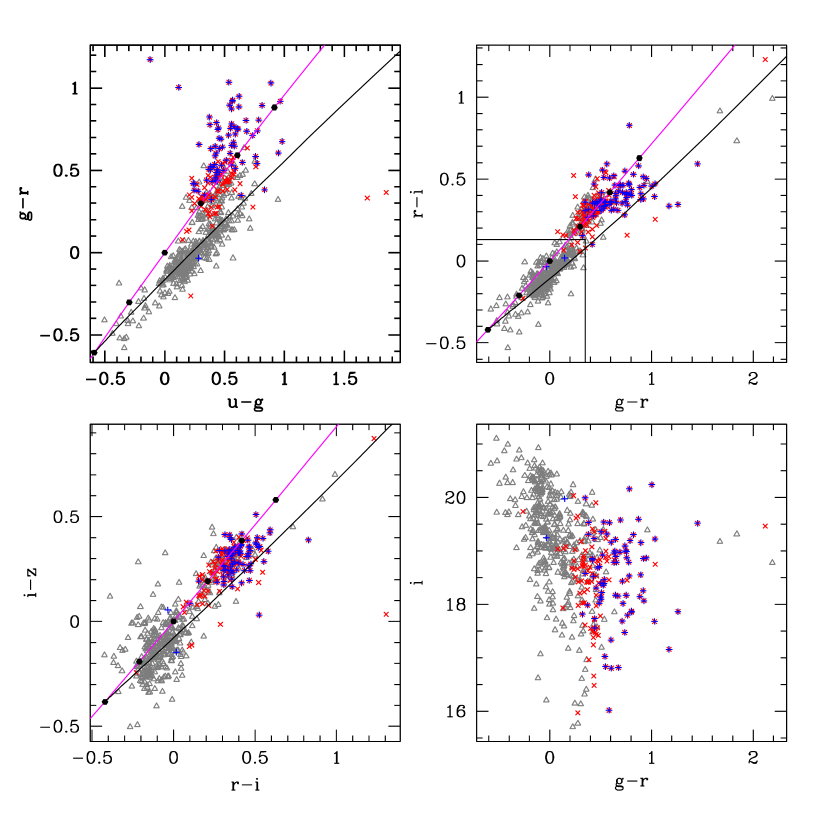
Figure 7: Similar to Figure 6, but broken up schematically according to image morphology and redshift. Grey triangles are objects with point-like morphologies and no identifiable spectral features for obtaining redshifts. Blue ‘+’ signs are resolved objects, and red ‘$\times$’ marks are objects with measured redshifts large enough to be cosmological; in many cases the latter two types of symbol overlap, especially for the reddest objects (those with strong host galaxy components). The localization of objects with redshifts or resolved morphologies is consistent with the separation according to proper motion that is apparent in Figure 6.

Figure 7 shows the same color-color diagrams as Figure 6, but the different symbols highlight objects with resolved morphologies or convincing cosmological redshifts (either from the pipeline or determined manually), that is, groups of objects that should be exclusively extragalactic in nature. The near-total absence of resolved objects or objects with redshifts in the blue-$gri$ region is rather striking, but in fact unsurprising, considering that significant host-galaxy starlight contributions (which enable most of our redshift measurements and are responsible for the extended morphologies) tend to move objects toward the red.

Of the 347 QFOs in the blue-$gri$ region, only five have measurable redshifts and only two are reported to be resolved by the SDSS photometric pipeline. The five blue-$gri$ objects with redshifts share the following other properties: (1) redshift (uncertain for three out of five) determined from weak broad emission lines rather than host galaxy absorption features; (2) unresolved optical morphology; and (3) proper motion either unreliable (2 objects) or $\mu<6$ mas yr^-1 (3 objects), well below our detection threshold. Two of these objects have FIRST counterparts, and one of these is also a RASS source. These are all very interesting objects, but the (possible) presence of broad emission lines, though weak, already hints that they may differ in a significant way from classical BL Lacs.

The two blue-$gri$ objects with resolved morphologies lack FIRST, NVSS and RASS counterparts, and they lack redshifts. Visual inspection of the images reveals that they are marginally resolved. These are the only QFOs in the sample that are spatially resolved but lack redshifts; we do not regard this as convincing evidence of an extragalactic nature.

4 Cross-correlations with X-ray and radio catalogs

4.1 ROSAT All Sky Survey (RASS)

We cross-correlated the full sample of quasi-featureless objects with the RASS bright and faint source catalogs (BSC, Voges et al. 1999; FSC, Voges et al. 2000). The RASS covers virtually the entire sky in the 0.1–2.4 keV range with a typical limiting sensitivity of $10^{-13}$ erg cm^-2 s^-1 and positional accuracy of 10–30 arcsec, for point sources. Using a matching radius of one arcmin, we find 65 matches in the BSC and 32 in the FSC. Based on a second search using a matching radius of five arcmin and applying a constant background model, we estimate the total expected number of mismatches within one arcmin to be significantly less than one for the BSC and approximately one for the FSC.

In order to convert the RASS count rates to approximate X-ray fluxes, we use the Portable Interactive Multi-Mission Simulator (PIMMS; Mukai 1993). We assume that the intrinsic X-ray spectrum in the (observed frame) energy range 0.1–2.4 keV is well-described by a power-law with frequency index $\alpha=1.25$ (i.e., $f_{\nu}\propto\nu^{-1.25}$), intermediate between typical values for low-redshift LBL and HBL objects (cf. Sambruna 1997). We modify the power-law spectrum according to the Galactic neutral hydrogen column density $N_{\mathrm{H}}$ toward each object, obtained using the FTOOLS (Blackburn, 1995) program NH, deriving the column density values from the maps of Stark et al. (1992). Adopting this absorbed power law as the input spectrum, we use PIMMS to convert from observed ROSAT PSPC count rate to flux density at 1 keV in the observed frame. For objects without counterparts in either the BSC or the FSC, we use the same procedure to place approximate upper limits on the 1 keV flux density, assuming count rates just below the FSC detection threshold (i.e., six counts divided by the exposure time appropriate for the object’s coordinates).

4.2 FIRST survey and NVSS

We also cross-correlated the sample of QFOs against the Faint Images of the Radio Sky at Twenty cm catalog (FIRST; Becker et al. 1995; White et al. 1997) and the NRAO/VLA Sky Survey (NVSS; Condon et al. 1998). The FIRST survey is designed to cover approximately the SDSS footprint area, with a typical sensitivity of one mJy at 1.4 GHz for point sources, a resolution of five arcsec, and sub-arcsec positional accuracy. The NVSS covers the whole sky north of declination $-40^{\circ}$ with a resolution of 45 arcsec, rms positional accuracy better than seven arcsec, and a typical limiting sensitivity of 2.5 mJy, also at 1.4 GHz.

We adopted a two arcsec matching radius for FIRST and a 10 arcsec radius for NVSS; optical/radio matching is discussed in detail by Ivezić et al. (2002). We find 183 and 198 matches in FIRST and NVSS respectively, within these radii. Of the 198 NVSS matches, 32 are not covered by FIRST; all the remaining 166 are detected by FIRST. Applying the same type of simple background analysis described in §4.1, the total expected number of mismatches using these matching radii is near zero for FIRST and approximately one for NVSS. Our choice of a 10 arcsec matching radius for NVSS is somewhat conservative; among our QFOs, there are two objects for which bright FIRST counterparts ($f_{\nu}>50$ mJy) exist within two arcsec of the SDSS position, but the nearest NVSS counterparts are separated by $>10$ arcsec from the SDSS position (12.2 and 25.4 arcsec separations), due to overlap with other nearby bright radio sources. However, the potential for confusion between SDSS and NVSS sources increases rapidly for matching radii $>10$ arcsec, and using a matching radius of 20 or 30 arcsec would result in numerous false matches.

In order to identify any likely FIRST counterparts with optical-to-radio separations greater than the matching radius of two arcsec (such as wide-separation double-lobed sources), we visually examined FIRST cutout images for all objects for which FIRST data were available at the time of writing. Only one additional likely FIRST match was discovered. The FIRST source has a somewhat unusual elongated radio morphology that approximately overlaps the SDSS position (J231952.82$-$011626.8) with a centroid separation of 3.2 arcsec; SDSS J2319$-$0116 (which is extended and shows strong host galaxy features) is the only apparent optical source in a SDSS mosaic image within five arcsec of the FIRST centroid position. There is also a RASS BSC source with a separation of four arcsec (well within the positional error) from SDSS J2319$-$0116. We consider SDSS J2319$-$0116 to be the likely source of both the X-ray and radio emission.

With very few exceptions, such as SDSS J2319$-$0116, FIRST counterparts of SDSS quasi-featureless objects clearly display compact core-dominated morphologies to the limit of the resolution of the FIRST survey. There are several instances of objects showing extended structures such as halos or weak one-sided jets, but no apparent lobe-dominated cases.

Where both FIRST and NVSS data exist, we use FIRST to take advantage of its significantly finer angular resolution. For all objects observed and not detected by FIRST, we use the FIRST non-detections to set upper limits on flux density at 1.4 GHz of $f_{\nu,\mathrm{lim}}=5\times f_{\nu,\mathrm{rms}}+0.25\mathrm{mJy}$, where $f_{\nu,\mathrm{rms}}$ is the noise level (typically $\approx 0.15$ mJy) appropriate to the object’s coordinates and 0.25 mJy is a correction for the CLEAN bias (e.g., Becker et al. 1995). For objects lacking FIRST data, we do not use NVSS non-detections to set upper limits due to the potential for confusion as discussed previously.

5 Properties of BL Lac candidates

Table 1 contains positions, SDSS photometric data, redshifts and proper motions for probable BL Lac candidates. Table 2 contains RASS, FIRST and NVSS data and derived quantities for probable BL Lac candidates. Tables 3 and 4 contain the analogous information for the possible BL Lac candidates.

5.1 Redshift distribution

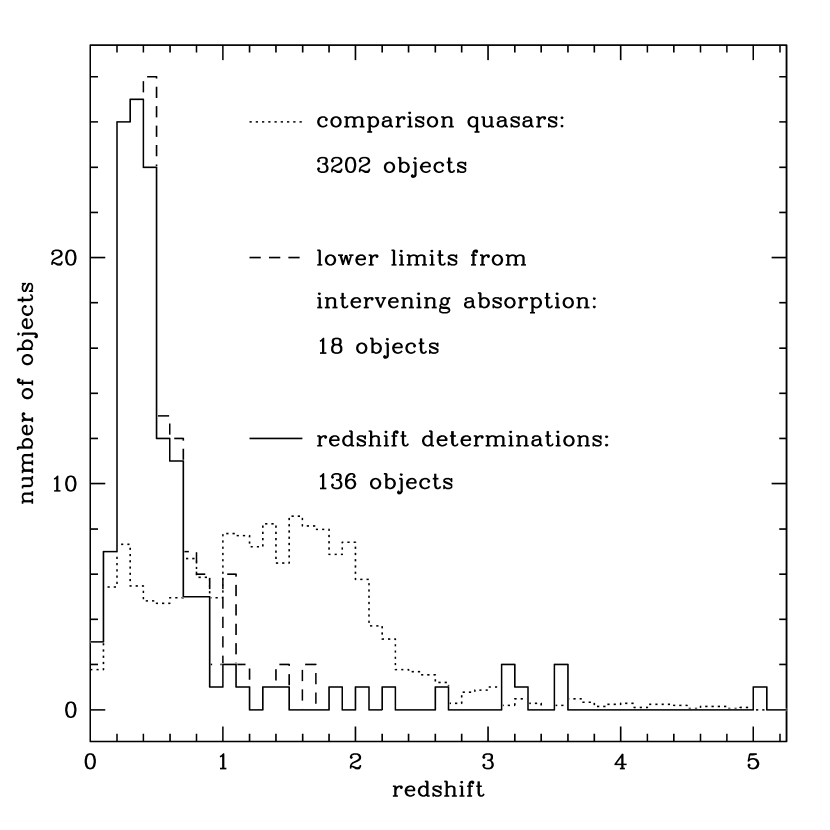
Figure 8: Redshift distributions for BL Lac candidates with measurable redshifts, as well as the sample of comparison quasars from §3.2.1. The solid line shows BL Lac candidates with emission-line or host-galaxy redshift determinations; the dashed line shows BL Lac candidates with redshift determinations plus those with redshift lower limits from intervening absorption. The dotted line shows the sample of comparison quasars (scaled down by a factor of approximately 20). The majority (232/386) of BL Lac candidates, including 86/240 probable candidates, are not shown due to the lack of redshift information.

Figure 8 shows the redshift distribution for the 154 BL Lac candidates with measurable redshifts or lower limits from intervening absorption; by definition these all fall into the “probable” category. The median measured redshift is 0.45. It is noteworthy that the redshift distribution of our BL Lac candidates extends out substantially farther than those for previous BL Lac samples (e.g., Stickel et al. 1991; Rector et al. 2000; Giommi et al. 2005). A handful of objects extend to high enough redshift ($\mathbf{z}\gtrsim 2.2$; $\mathbf{z}_{\mathrm{max}}=5.03$) that Ly$\alpha$ enters the observed wavelength range; these objects invariably show at least hints of weak, broad Ly$\alpha$ emission lines (typically with observed $EW>5$ Å but $RFEW<5$ Å), as in Figure 3b. Some of these high redshift BL Lac candidates, along with similar objects discovered in high redshift quasar searches (Fan et al., 1999; Anderson et al., 2001), may in fact represent the low-EW tail of the normal quasar (high-luminosity AGN) population rather than true BL Lacs. All of the nine BL Lac candidates with $\mathbf{z}>2$ lack RASS counterparts, and six of them also lack FIRST/NVSS counterparts; thus it is difficult at present to confirm or reject this hypothesis (but see discussion in §5.6). This possibility, in addition to the large sample size, may explain the apparent discrepancy in redshift distributions.

Of the BL Lac candidates with no redshift information, those that are truly extragalactic are likely to populate the redshift range $0.5\lesssim\mathbf{z}\lesssim 2.2$; lower than $\mathbf{z}\sim 0.5$, host galaxy features should generally be apparent even in moderate $S/N$ spectra, and at $\mathbf{z}>2.2$, the Ly$\alpha$ forest would enter the spectra. Also shown in Figure 8 is the observed redshift distribution of the comparison quasar sample, which is close to flat out to $\mathbf{z}\sim 2$. Bearing in mind that a large fraction of the BL Lac candidates lacking redshifts are likely to be DC WDs, it would be impossible to make the BL Lac candidate redshift distribution match the comparison quasar redshift distribution up to $\mathbf{z}\sim 2$, even with appropriate choices of redshift for the BL Lac candidates with unknown redshifts or redshift limits. This is qualitatively consistent with a picture in which BL Lacs are (on average) low-luminosity AGNs, and their higher-luminosity counterparts, the FSRQs, do not necessarily share the property of having emission lines that are weak with respect to the beamed continuum radiation (e.g., Urry & Padovani 1995).

5.2 Optical colors of objects with X-ray and radio counterparts

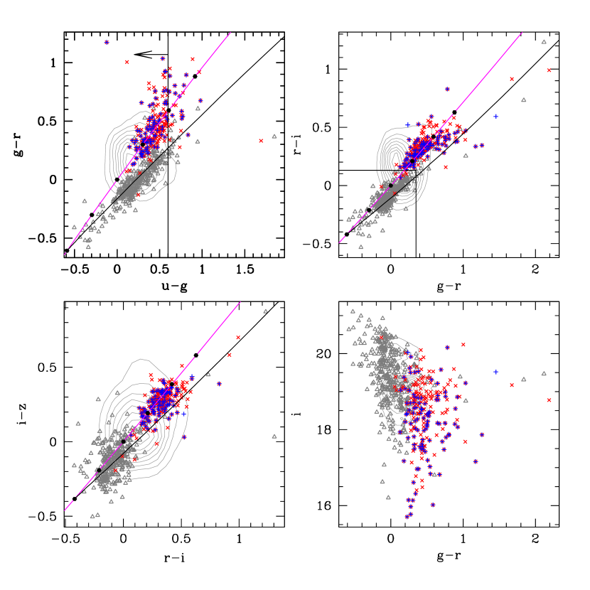
Figure 9: Similar to Figure 6, but broken up schematically according to radio and X-ray detections rather than proper motion. Contours represent the comparison quasar sample (see §3.2.1). Grey triangles are QFOs with neither FIRST/NVSS nor RASS counterparts. Blue ‘+’ symbols and red ‘$\times$’ marks are QFOs with RASS or FIRST/NVSS detections, respectively (in many cases they overlap). The QFOs with X-ray and/or radio detections lie almost exclusively outside the region of color space populated by objects with significant proper motions (see Figure 6).

Figure 9 shows the same color-color diagrams as Figure 6, symbolically coded according to X-ray and radio detections. Out of 97 RASS matches, only one lies in the blue-$gri$ region of color space. Out of 184 FIRST matches, only six lie in the blue-$gri$ region of color space. Out of 32 objects with NVSS matches and no FIRST coverage, only one lies in the blue-$gri$ region. For comparison, 347/580$=59.8$% of all QFOs lie in the blue-$gri$ region of color space; after the proper motion cut, 156/386$=40.4$% of BL Lac candidates still lie in this region. By contrast, there are only 22 QFOs outside the blue-$gri$ region that do not have FIRST or NVSS counterparts. This simultaneously emphasizes that outside the blue-$gri$ region, there is not much room for contamination by DC WDs, and reinforces the notion that true BL Lacs with such blue optical colors are much rarer than “normal” BL Lacs.

5.3 Subdividing the sample

Primarily because we do not have reliable proper motion measurements for 246 QFOs, the sample of 386 BL Lac candidates remains significantly contaminated by DC white dwarfs. The observed color separation in Figures 6, 7 and 9, between objects with significant proper motions and objects with low proper motions or other evidence of an extragalactic/AGN nature (radio or X-ray detections or redshifts), argues strongly that most true BL Lac lie outside the blue-$gri$ region, while most DC WDs lie within it. Within the blue-$gri$ region there are a total of 10 QFOs that show evidence of a likely extragalactic/AGN nature; outside the blue-$gri$ region there are a total of 11 QFOs that lack such evidence (plus an additional three rejected by the proper motion cut). Indeed, all available data are consistent with the more ambitious proposal put forward in §3.2.2, that nearly all the QFOs within the blue-$gri$ region are stars whereas nearly all the QFOs outside the blue-$gri$ region are extragalactic.

Based on this compelling argument, and in order to minimize the impact of the remaining DC WD contamination, we subdivide the sample into “probable” BL Lac candidates and “possible” BL Lac candidates. Here “probable” signifies a probable extragalactic nature (though not necessarily classical BL Lac status) and “possible” signifies a likely stellar nature. We define probable BL Lac candidates to be those objects that (1) lie outside the blue-$gri$ region of color space (i.e., $g-r\geq 0.35$ or $r-i\geq 0.13$) or (2) have X-ray or radio counterparts or measured redshifts. We define possible BL Lac candidates to be everything else, that is, objects that lie within the blue-$gri$ region and have no indication of extragalactic nature (X-ray/radio counterparts or redshifts).

By these definitions, we have 240 probable and 146 possible BL Lac candidates. Of the 39 Kleinman et al. (2004) objects that qualify as BL Lac candidates, 38 fall into the possible category; the remaining object also lies within the blue-$gri$ region, but has an apparent FIRST counterpart. Thus we conclude that the probable BL Lac candidates are not appreciably contaminated by previously known white dwarfs. For the possible BL Lacs, we offer a word of caution: if there exist quasi-featureless extragalactic objects (no spectral features detected with the SDSS spectral $S/N$) that are weak compared to classical BL Lacs in X-ray and radio (undetected by RASS and FIRST/NVSS) and have bluer-than-average optical colors (within the blue-$gri$ region), they would fall into the possible category. Although we argue that most if not all of the possible BL Lac candidates are likely to be stars, a more detailed analysis of the statistics of DC WD proper motions and number counts would be required in order to prove that this is the case. Such an analysis is beyond the scope of the present work.

5.4 BL Lac colors and number counts

Adopting the conclusion that very few or none of the possible BL Lac candidates are in fact BL Lacs, we note that the colors of the true BL Lacs in our sample (the probable candidates) are 0.2–0.4 mag redder on average than the comparison quasars, shown as contours in Figure 9. Starlight from BL Lac host galaxies can contribute to this effect, if the (apparent) AGN/host-galaxy luminosity ratio is lower for BL Lacs than for quasars, as expected if BL Lacs are on average relatively low luminosity AGNs. However, subtracting the host galaxy contributions cannot even approximately account for the differences in the average colors, so we conclude that the intrinsic power-law (host galaxy subtracted) spectra of our true BL Lacs are redder on average than the intrinsic (thermal/disk plus non-thermal) spectra of quasars.

If we assume that the probable BL Lacs form a statistically complete sample to $i\approx 19$ (just brighter than the magnitude limit for low-redshift SDSS quasar spectroscopic target selection) and take into account that most of the probable candidates (all of those with $i<19$) have $g-i>0.2$, then the sample is complete to at least $g\approx 19.2$. (This may be a bad assumption because the sample may not be complete, or because not all objects in the sample may be true BL Lacs, but fortunately these two effects are of opposite sign.) There are 98 probable BL Lac candidates with $g<19.2$, selected out of 2860 deg² of sky, yielding a surface density of 0.034 deg^-2 brighter than this limit. If one is willing to make the additional assumption that $g\sim B$, this number may be compared with the number count extrapolations in Figure 2 of Padovani & Urry (1991); they are mutually compatible, albeit with a large range of uncertainty. For comparison, there are $\sim 4$–5 quasars deg^-2 to the same limiting magnitude (e.g., Boyle et al. 2000).

5.5 SDSS target selection effects

The majority (349/386) of our BL Lac candidates, including 205/240 of the “probable” candidates, have dereddened $u-g<0.6$ (marked in the upper left panel of Figure 9), i.e., they satisfy the UVX criterion of SDSS low-redshift quasar target selection. Out of 386 total BL Lac candidates, 225 are targeted by low-redshift quasar target selection, including 179/240 probable candidates. The remainder of the candidates either have colors similar to WDs (and are therefore excluded from quasar target selection; Richards et al. 2002) or are simply too faint. The same UVX criterion provides grounds for inclusion in the blue-serendipity targeting routine as well; although this selection route receives lower priority than the main target selection routines, it populates parts of color-space that might otherwise be ignored (such as the WD exclusion region), and extends to a fainter limiting magnitude than low-redshift quasar targeting. Blue-serendipity targeting accounts for an additional 106 BL Lac candidates, including 10 probable ones. The remaining 55 BL Lac candidates (including 51 probable ones) are mostly targeted due to their radio or X-ray properties.

5.6 Radio-optical and optical-X-ray slopes

For the purpose of calculating broad-band radio-to-optical and optical-to-X-ray spectral slopes ($\alpha_{\mathrm{ro}}$ and $\alpha_{\mathrm{ox}}$) that can be readily compared with those appearing in other works, we adopt standard (rest-frame) reference frequencies of 5 GHz=6 cm, $6\times 10^{14}$ Hz=5000 Å and $2.42\times 10^{17}$ Hz=1 keV. Since we do not have observations covering these rest-frame frequencies in all cases (most notably near 5 GHz where we have essentially no data, the nearest observed frequency being 1.4 GHz from FIRST/NVSS), this procedure necessarily requires some assumptions and extrapolations. We assume that the radio, optical and X-ray spectra are locally power laws $f_{\nu}\propto\nu^{-\alpha}$ with exponents $\alpha_{\mathrm{r}}=-0.27$ (the average value for the 1 Jy sample; Stickel et al. 1991), $\alpha_{\mathrm{o}}=1.5$ (typical of the probable BL Lac candidates) and $\alpha_{\mathrm{x}}=1.25$ (see §4.1). To objects that lack redshift information, we assign the median measured redshift (0.45) if they fall into the probable category, or zero if they fall into the possible category; uncertain redshifts and redshift lower limits are treated as secure redshift measurements for this calculation. We normalize the assumed radio and X-ray spectra using the 1.4 GHz and 1 keV (observed frame) data points. After correcting the optical magnitudes for the Galactic extinction derived from the Schlegel, Finkbeiner, & Davis (1998) map, we normalize the assumed optical spectrum using the nearest in wavelength to rest-frame 5000 Å of the $g,r,i,z$ magnitudes (depending on redshift).

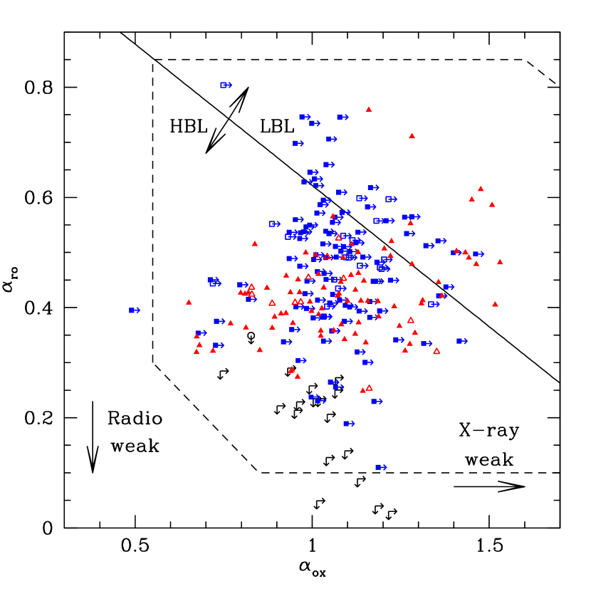
Figure 10: X-ray-optical-radio color-color diagram for probable BL Lac candidates. The parameters $\alpha_{\mathrm{ox}}$ and $\alpha_{\mathrm{ro}}$ are defined in the rest frame with the sign convention $f_{\nu}\propto\nu^{-\alpha}$, using reference points at 5 GHz, 5000 Å and 1 keV as described in the text in §5.6. The dashed line approximately encloses the population of known BL Lacs (e.g., Fig. 1 of Perlman et al. 2001). The slanted line shows the formal division between HBL-type and LBL-type objects at $\alpha_{\mathrm{rx}}\approx 0.75$ (e.g., Padovani & Giommi 1995). Red triangles are objects with both radio (FIRST=solid or NVSS=outline) and X-ray (RASS) detections; blue squares with arrows are objects with radio detections and X-ray upper limits. The black circle is the lone object with a RASS detection and a FIRST upper limit. Pairs of arrows represent objects with upper limits in both radio and X-rays. There are substantial uncertainties in the locations of objects on this diagram (see §5.6).

Figure 10 shows an X-ray-optical-radio color-color diagram ($\alpha_{\mathrm{ox}},\alpha_{\mathrm{ro}}$) for probable BL Lac candidates. There are uncertainties in the locations of individual objects on this diagram, mainly due to (1) non-simultaneity of observations at different frequencies, which is a concern because of BL Lac variability, (2) uncertainties introduced in the procedure of converting RASS count rates to flux, and (3) non-detection of many objects at X-ray or radio frequencies. Moreover, since we have assumed uniform X-ray, optical and radio power-law slopes to extrapolate observed data points to rest-frame reference frequencies, the true scatter in the plot is probably under-represented. We note that Figure 10 qualitatively differs from the analogous Fig. 3 of Collinge et al. (2004), due to the more sophisticated procedure for calculating X-ray fluxes and broad-band spectral slopes; this simply serves to emphasize the potential for confusion.

It is nevertheless apparent that the sample follows a more-or-less continuous distribution of properties from high-energy peaked (HBL) toward low-energy peaked (LBL) SEDs, with no shortage of intermediate-type objects. This behavior is characteristic of the blazar class (Perlman et al., 1998, 2001), despite previous and by now historical indications of a gap between HBL and LBL type objects (e.g., Padovani & Giommi 1995), which resulted from the very different selection biases imposed on radio versus X-ray selected samples. Perhaps the most noteworthy feature of Figure 10 is that all the objects with X-ray or radio detections fit so comfortably within the range of properties of previously-known BL Lacs (e.g., Fig. 1 of Perlman et al. 2001), despite the large sample size and relatively novel selection biases. If there are any BL Lac candidates in our sample with exceptionally weak radio or X-ray emission, then they must appear in Figure 10 only as limits or fall into the possible category (see discussion in §5.3). Among classical BL Lacs, the lowest known values of $\alpha_{\mathrm{ro}}$ are in the neighborhood of 0.1 (cf. Fan et al. 1999); four of our candidates have upper limits on $\alpha_{\mathrm{ro}}$ below this level. Because our derived $\alpha_{\mathrm{ro}}$ values are somewhat uncertain, we separate out all probable BL Lac candidates with $\alpha_{\mathrm{ro}}<0.2$ (8 objects) or no radio detections (another 19 objects). We present these 27 candidates in Table 5; deeper radio observations of these objects are needed in order to understand the radio-weak tail of the BL Lac population.

In addition to the broadband spectral slope $\alpha_{\mathrm{ro}}$, another parameter that has been used to discriminate between radio-loud and radio-quiet AGN is the luminosity density at radio frequencies (e.g., Stocke et al. 1992); these authors placed the dividing line at $L_{\nu}\sim 10^{33}$ erg s^-1 Hz^-1 for $\mathbf{z}\sim 2$ quasars. This number was obtained assuming an $H_{0}=50$ km s^-1 Mpc^-1, $\Omega_{\mathrm{total}}=\Omega_{\mathrm{m}}=1$ cosmology, as opposed to the currently favored “concordance” $H_{0}=70$ km s^-1 Mpc^-1, $\Omega_{\mathrm{m}}=0.3$, $\Omega_{\Lambda}=0.7$ model. Conveniently, these different cosmological models yield nearly equivalent (consistent to about 2%) luminosity distance scales at $\mathbf{z}=2$ (the concordance model gives a slightly longer distance), so in practice no conversion is required. Assuming the concordance cosmology, all of the objects in Table 5 for which we have radio constraints fall below the approximate $L_{\nu}\sim 10^{33}$ erg s^-1 Hz^-1 dividing line. While we do not advocate this approach to determining radio-loud/radio-quiet nature, this analysis provides another useful benchmark.

Bearing in mind the uncertainties in our derived values of $\alpha_{\mathrm{ox}}$ and $\alpha_{\mathrm{ro}}$, HBL or intermediate objects appear to constitute the majority of our sample. This may seem unsurprising, considering that the gap between the optical and soft X-ray bands is less than three orders of magnitude in frequency, while the gap between optical and radio is more like five. However, we note that the range of synchrotron peak frequencies $\nu_{\mathrm{peak}}$ of BL Lac objects is thought to be approximately $10^{13}\mathrm{Hz}<\nu_{\mathrm{peak}}<10^{18}\mathrm{Hz}$ (e.g., Antón & Browne 2004), with LBLs at the low end and HBLs at the high end. Based on the experience of previous BL Lac searches — “the surveys find what they can rather than what exists” (Padovani & Urry, 2001) — we expected that our sample would be biased toward objects with $\nu_{\mathrm{peak}}$ close to the optical (i.e., toward the low end of the $\nu_{\mathrm{peak}}$ range), and thus dominated by LBLs. Uncertainties in ($\alpha_{\mathrm{ox}},\alpha_{\mathrm{ro}}$) notwithstanding, this is evidently not the case.

A strong selection effect that may contribute to a HBL-bias is the SDSS quasar target selection UVX cut (dereddened $u-g<0.6$), which most of our BL Lac candidates satisfy, as discussed in §5.5. Figure 9 shows that the numbers of BL Lac candidates drop sharply for $u-g>0.6$. Thus, most of our sample may be considered UVX-selected. Although the SDSS $u$-band is centered at $\nu_{\mathrm{eff}}\approx 8.51\times 10^{14}$ Hz (still toward the low end of the $\nu_{\mathrm{peak}}$ distribution), the requirement imposed on UV continuum slope may result in a bias toward HBL-type objects.

5.7 Comparison with Anderson et al. (2003)

Anderson et al. (2003) presented a sample of candidate BL Lacs selected as part of a project to use SDSS imaging and spectroscopy to obtain optical identifications of a large sample of RASS X-ray sources. Their sample contained 38 “probable” (by their own definition) and seven additional “possible” (by their own definition) BL Lacs selected from 1400 deg² of SDSS data. This area of sky is covered by the spectroscopic parent sample for our search. Of the 38 Anderson et al. (2003) probable BL Lacs, our search recovers 35 objects; one of the remaining three objects fails the $S/N$ requirement (see §3.1.1), and the other two fail the polynomial test (these objects are classified as galaxies; see §3.1.2). We also recover two out of the seven Anderson et al. (2003) possible BL Lacs. All the Anderson et al. (2003) objects that we recover are categorized (according to our definition) as probable BL Lacs due to their X-ray counterparts.

Following Anderson et al. (2003), we calculate the X-ray to optical flux ratio $f_{\mathrm{x}}/f_{\mathrm{opt}}$, where $f_{\mathrm{x}}$ is the broadband absorption-corrected X-ray flux in the observed frame energy range 0.1–2.4 keV, and $f_{\mathrm{opt}}$ is the broadband extinction-corrected optical flux in the observed frame wavelength range 4000–9000 Å. As in Anderson et al. (2003) we assume the X-ray and optical spectra to be power laws $f_{\nu}\propto\nu^{-\alpha}$ with $\alpha_{\mathrm{x}}=1.5$ and $\alpha_{\mathrm{opt}}=0.5$. The value of $\alpha_{\mathrm{x}}$ assumed here differs by 0.25 from that which we employed in §4.1. The choice of $\alpha_{\mathrm{opt}}=0.5$ is representative of the sample of QFOs as a whole (see Figure 6), though they span a relatively large range ($\gtrsim 3$) in $\alpha_{\mathrm{opt}}$; our probable BL Lac candidates are actually shifted toward steeper (redder) slopes as discussed in §3.2.2 and 5.6. We set the normalizations of the X-ray and optical power laws using the flux densities at 1 keV (cf. §4.1) and in the $g$-band ($\nu_{\mathrm{eff}}\approx 6.36\times 10^{14}$ Hz).

Distributions of $f_{\mathrm{x}}/f_{\mathrm{opt}}$ for several subsets of BL Lac candidates are shown in Figure 11. The lowermost histogram may be compared with the lower panel of Fig. 10 from Anderson et al. (2003) (not shown); the Anderson et al. (2003) distribution extends to a slightly higher value of $f_{\mathrm{x}}/f_{\mathrm{opt}}$. This probably reflects the different selection biases at work; if the eight Anderson et al. (2003) objects not included in our sample are fainter at optical wavelengths, they will tend to be biased toward X-ray dominated objects, for a fixed X-ray sensitivity. In any case, it is interesting that all three distributions in Figure 11 and that from Anderson et al. (2003) peak at similar values of $f_{\mathrm{x}}/f_{\mathrm{opt}}$, suggesting a broad similarity in the properties of the X-ray-selected Anderson et al. (2003) sample and our (largely) optically-selected sample. This is consistent with the result from the previous section that the majority of our objects appear to be HBL-type.

6 Future work

The sample of BL Lac candidates presented in this paper is ripe for further analysis and future work. In particular:

• None of the BL Lac candidates with radio or X-ray counterparts stand out from the range of properties of previously known BL Lacs. Our ability to constrain the relative abundances of anomalously X-ray or radio-quiet BL Lacs is currently limited by the sensitivity of available X-ray and radio observations; thus deeper observations at these frequencies are needed.

• With higher-$S/N$ spectroscopy of some of the objects that currently lack redshift measurements, it would be possible to construct the luminosity function of BL Lacs, and by comparing this with the luminosity functions of other radio-loud AGN, constrain models for jet opening angles as a function of luminosity. Carrying out this calculation will require a full understanding of the selection function of the sample imposed by the SDSS color selection (§5.5). For unreddened BL Lacs at $\mathbf{z}<2$, this is reasonably straightforward, given the high completeness of the blue selection of SDSS quasars (Richards et al., 2002; Vanden Berk et al., 2004b).

• It will also be important to quantify the incompleteness of the sample due to our strict rejection of objects with emission lines. There should be BL Lacs whose host galaxies contain H II regions, giving rise to emission lines of high enough EW to cause objects to be rejected from the sample. There is also some inevitable incompleteness at the low-luminosity end arising from our requirement that the non-thermal continuum be $>50\%$ of the spectrum at either the blue or red end, as well as from our requirements on $S/N$.

• One of the ways in which BL Lacs manifest themselves is by their variability. SDSS provides separate observations of these objects in the SDSS imaging and spectroscopy, which, as Vanden Berk et al. (2004a) show, can be used to explore the statistical properties of the variability of the population. Some patches of the survey area have multiple imaging scans as well. It will be interesting to see how our optically selected BL Lac candidates compare in this respect with previously known BL Lacs.

• Polarization is another defining characteristic of the BL Lac population. We have no information about the optical polarization properties of the sample, but the objects are reasonably bright, with $i_{\mathrm{med}}=18.95$, so a broad-band polarization survey of a well-defined subset of the objects, especially those at higher redshifts, would be straightforward and informative.

• Finally, the DC white dwarfs which we have culled from the sample are interesting in their own right (Kleinman et al., 2004). Their proper motions and brightnesses allow calculation of crude distances, and thus a determination of their luminosity function and a comparison with the population of cooler white dwarfs. This may be important for models of white dwarf formation and cooling.

7 Conclusions

We present a large sample of candidate BL Lacertae objects from the spectroscopic database of the Sloan Digital Sky Survey. BL Lacs are rare AGNs in which the dominant source of observed radiation is thought to be a relativistic jet of plasma directed within a small angle to the line of sight, and in which the broad emission lines typical of unobscured AGNs are weak or washed out. While the latter trait is not well understood, the upshot is that BL Lacs have nearly featureless optical spectra; we use this property as the basis of our selection criteria. We define an object to have a quasi-featureless spectrum if it: (1) has no identified emission lines with rest-frame equivalent width $RFEW>5$ Å; (2) shows no evidence of stellar absorption features at zero redshift; (3) is not well-fit by stellar templates or combinations of galaxy eigenspectra; and (4) has Ca II H&K break strength $C\leq 0.4$, for $|C/\delta C|>3$. (Certain extreme objects such as some broad-absorption-line quasars formally fulfill these requirements; such “messy” spectra are rejected as well.)

The primary astrophysical contaminants among quasi-featureless objects (QFOs) are DC white dwarfs. We have found (following Londish et al. 2002) that these can largely be rejected based on their high proper motions, although a significant fraction of objects lack reliable proper motion measurements, and hence a large degree of contamination remains in our sample. Out of 580 originally-selected QFOs, the 386 final BL Lac candidates are chosen to be those objects with low or unreliable proper motions. Only 85 of the objects in the sample have been previously reported as BL Lacs in the NASA/IPAC Extragalactic Database (NED). The sample is drawn from approximately 2860 square degrees of sky ($\sim 1/3$ of the complete SDSS) and has a median $i$ magnitude of 18.95.

We have been able to measure or constrain redshifts for 154/386 of our BL Lac candidates, either from stellar absorption lines, or in a few cases, by using intervening absorption systems to place lower limits. The majority of these objects (131) have redshifts less than unity (the median measured redshift is $\mathbf{z}_{\mathrm{med}}=0.45$), with a tail of objects extending out to high redshift ($\mathbf{z}_{\mathrm{max}}=5.03$). These high redshift objects are potentially weak-lined normal quasars (as opposed to true BL Lacs), like those discussed by Fan et al. (1999) and Anderson et al. (2001) (but our sample does not include those specific objects due to the details of our selection criteria). The remaining true BL Lacs in the sample are likely to have redshifts in the approximate range $0.5\lesssim\mathbf{z}\lesssim 2.2$.

We searched for X-ray and radio counterparts to QFOs using the ROSAT All-Sky Survey X-ray source catalogs and the FIRST and NVSS radio catalogs. On optical color-color diagrams, featureless objects with high proper motions tend to be confined in color space, generally following the loci of blackbody colors as a function of temperature (typically 7000–12000 K). QFOs with redshifts or X-ray or radio counterparts (i.e., evidence of an extragalactic/AGN nature) almost exclusively lie outside the region of color space containing high-proper-motion objects. In fact, the optical colors of apparently-extragalactic QFOs are reasonably well-described in terms of power-law spectra (typically $1<\alpha_{\mathrm{opt}}<2$) plus host galaxy starlight rather than blackbodies. We conclude that most of the 156 remaining BL Lac candidates with blackbody-like colors are in fact DC white dwarfs, either with low proper motions or too faint to have reliable proper motion constraints. To restrict the impact of this significant contamination on our results, we divide the sample into 240 “probable” (i.e., likely extragalactic) candidates, with colors unlike those of DC WDs or other evidence of extragalactic/AGN nature (redshift or radio/X-ray counterparts), and 146 “possible” (i.e., likely stellar) candidates, with colors consistent with the high proper motion objects, and no other evidence of extragalactic/AGN nature. The probable BL Lac candidates have colors generally consistent with the ranges of known quasar colors, but on average are redder by $\sim 0.2$–0.4 mag, plus a redder tail of objects with more significant host galaxy contributions.

Despite the large sample size and relatively novel selection biases, we find that the multi-wavelength properties of our probable BL Lac candidates do not systematically deviate from the range of properties of previously known BL Lacs. The majority of our BL Lac candidates detected in both X-ray and radio wavebands are consistent with being high-energy synchrotron-peaked (i.e., HBL/XBL type) objects, which may be due to a HBL-bias introduced by the UV-excess requirement ($u-g<0.6$) of SDSS low-redshift quasar spectroscopic target selection. Given the sensitivities of the RASS and FIRST/NVSS catalogs with which we compare, we find little evidence for a population of extragalactic objects with featureless optical spectra, that are under-luminous in either X-rays or radio. We present a list of the 27 most promising candidate radio-weak BL Lacs (though only eight currently have limits $\alpha_{\mathrm{ro}}<0.2$); more sensitive radio observations are needed for these objects before we can make a strong statement about the abundance of radio-quiet quasi-featureless AGN.

Figure 1: Example weak-featured SDSS spectra. The smooth solid curves show the polynomial components from the pipeline spectral fits. The feature at 5577 Å, most prominent in panels (b) and (c), is a residual from sky subtraction. Two out of the three objects were mis-classified by the spectral pipeline and assigned erroneous redshifts; in all three cases redshift warning flags were set. The dotted vertical lines mark the positions of apparent absorption features. Panel (a): no features are detected; this object survives the stellar absorption line cut described in §3.1.2 and enters the sample of QFOs. Panel (b): He I $\lambda\lambda$ 4026, 4471, 5876 Å are detected in absorption; thus this object is probably a DB WD. Panel (c): shallow Swan bands of the C₂ molecule are detected (dotted lines mark their approximate edges); this object is a DQ WD. Objects (b) and (c) are rejected as QFOs.

Figure 3: Example SDSS marginal emission-line objects, similar to Figs. 1 and 2. Dotted lines again mark absorption features, and dashed lines mark emission features. All three spectra show significant sky residuals at the red ends; many of the apparent emission features long-ward of about 7500 Å cannot be trusted. Panel (a): the broad emission-line-like feature observed near 5630 Å may be Mg II $\lambda$ 2800 Å; however, the identification is not secure primarily due to the lack of other features, so this object survives the emission line cut described in §3.1.3 and enters the sample of QFOs. Panel (b): the broad lines appear weak and/or absorbed in this object; the C IV $\lambda$ 1549 Å line (observed near 6800 Å and possibly blue-shifted with respect to Ly$\alpha$) has RFEW close to 5 Å, but with substantial uncertainty. Therefore object (b) survives as a QFO. Panel (c): O II $\lambda$ 3727 Å has RFEW$>$5 Å. Object (c) is rejected as a QFO.

Figure 4: Distribution of measured proper motions for 2092 spectroscopically confirmed SDSS quasars. Proper motions are obtained from the Munn et al. (2004) catalog, extended to include SDSS objects not in DR1, and are required to satisfy reliability criteria as described in §3.2.1. The vertical dashed line marks $\mu=11$ mas yr^-1; 95.0% of the quasars have measured proper motions below this level.

Figure 5: Reliably measured proper motions vs. $r$-band magnitude for comparison quasars and quasi-featureless objects. Horizontal dashed lines mark the 11 mas yr^-1 level; for clarity, only 500 of the comparison quasars (randomly selected) are shown.

Figure 11: Histograms of $\log(f_{\mathrm{x}}/f_{\mathrm{opt}})$ for three subsets of BL Lac candidates. The bin size is 1/3 dex, and the middle and uppermost histograms are vertically offset for clarity by 0.5 and 1.0 respectively. The quantities $f_{\mathrm{x}}$ and $f_{\mathrm{opt}}$ are calculated as described in §5.7. The lowermost histogram may be compared with the lower panel of Fig. 10 from Anderson et al. (2003). The uppermost histogram consists of upper limits on $\log(f_{\mathrm{x}}/f_{\mathrm{opt}})$ (see §4.1) for probable BL Lac candidates undetected in the RASS BSC and FSC.

Table 1: SDSS photometric and spectroscopic measurements, proper motions, and previous identifications for “probable” BL Lac candidates.

	$u$	$g$	$r$	$i$	$z$	Ar 1	Optical	Target		$\mu$	Previously
IAU designation	(mag)	(mag)	(mag)	(mag)	(mag)	(mag)	morph.	code	Redshift	(mas yr-1)	identified?
(1)	(2)	(3)	(4)	(5)	(6)	(7)	(8)	(9)	(10)	(11)	(12)
SDSS J012227.38$+$151023.1	20.34$\pm$0.05	19.90$\pm$0.02	19.55$\pm$0.03	19.25$\pm$0.03	18.93$\pm$0.05	0.17	p	1048580	$\cdots$	7.1	N
SDSS J012716.31$-$082128.9	20.26$\pm$0.07	19.70$\pm$0.03	19.14$\pm$0.03	18.81$\pm$0.02	18.55$\pm$0.04	0.08	p	20	0.362?	4.1	Y
SDSS J012750.83$-$001346.6	21.03$\pm$0.09	20.66$\pm$0.04	19.83$\pm$0.02	19.30$\pm$0.03	18.95$\pm$0.04	0.09	r	2097154	0.4376	6.0	N
SDSS J013408.95$+$003102.5	21.17$\pm$0.10	20.22$\pm$0.03	19.90$\pm$0.02	19.72$\pm$0.03	19.79$\pm$0.08	0.07	p	2	$\cdots$	154.5?	N
SDSS J014125.83$-$092843.7	18.11$\pm$0.02	17.59$\pm$0.03	17.21$\pm$0.02	16.96$\pm$0.01	16.68$\pm$0.02	0.08	p	7700	$\geq 0.5$?	5.8	Y
SDSS J020106.18$+$003400.2	18.90$\pm$0.02	18.62$\pm$0.02	18.25$\pm$0.03	17.99$\pm$0.02	17.80$\pm$0.02	0.07	r	5636	0.2985	7.6	Y
SDSS J020137.66$+$002535.1*	20.39$\pm$0.05	20.06$\pm$0.02	19.54$\pm$0.02	19.39$\pm$0.02	19.38$\pm$0.09	0.08	p	1048576	$\cdots$	176.1?	N
SDSS J022048.46$-$084250.4	18.92$\pm$0.02	18.62$\pm$0.03	18.27$\pm$0.02	18.03$\pm$0.02	17.80$\pm$0.03	0.06	p	1056276	0.5252?	7.1	N
SDSS J023813.68$-$092431.4	20.86$\pm$0.09	20.27$\pm$0.03	19.63$\pm$0.02	19.22$\pm$0.03	18.85$\pm$0.05	0.08	r	2102788	0.4188	3.6	Y
SDSS J024156.38$+$004351.6	20.66$\pm$0.08	20.03$\pm$0.02	19.61$\pm$0.02	19.41$\pm$0.03	19.29$\pm$0.05	0.09	p	3	0.99	6.1?	N

Note. — Positions are in J2000 coordinates. Photometric measurements are reported in PSF magnitudes, not corrected for the Galactic extinction. The symbol ‘*’ following the IAU designation indicates that the SDSS data using DR2 reductions were not available for the object; the data reported are from the DR1 reductions. The abbreviation ‘p’ in column (8) indicates that the object is point-like in the SDSS image; ‘r’ indicates that it is resolved. Column (9) reports the SDSS primary spectroscopic target code, in which each (binary) bit represents a flag for a different targeting algorithm; see Stoughton et al. (2002) for a list of the different targeting algorithms and their corresponding bits. A question mark ‘?’ following the entry in column (10) or column (11) indicates that the redshift is uncertain or the proper motion is deemed to be unreliable, respectively. Column (12) indicates whether the object was previously reported in NED as a BL Lac. The full version of this table will be published online in the Astronomical Journal.

References. — (1) Derived from Schlegel, Finkbeiner, & Davis (1998)

Table 2: Multi-wavelength data for “probable” BL Lac candidates.

		ROSAT All-Sky Survey						FIRST			NVSS
IAU designation	$N_{\mathrm{H}}$	match	sep.	count	exp.	$f_{\mathrm{E}}$(1keV)	$f_{\mathrm{x}}$	sep.	$f_{\nu}$(1.4GHz)	$f_{\mathrm{rms}}$	sep.	$f_{\nu}$(1.4GHz)	$\alpha_{\mathrm{ox}}$	$\alpha_{\mathrm{ro}}$
	($10^{20}$cm-2)		(arcsec)	rate (s-1)	(s)			(arcsec)	(mJy)	(mJy)	(arcsec)	(mJy)
(1)	(2)	(3)	(4)	(5)	(6)	(7)	(8)	(9)	(10)	(11)	(12)	(13)	(14)	(15)
SDSS J012227.38$+$151023.1	4.29	U	$\cdots$	$<$0.03	178.2	$<$5.7	$<$25.7	$\cdots$	$\cdots$	$\cdots$	0.8	38.0$\pm$1.2	$>$0.90	0.50
SDSS J012716.31$-$082128.9	3.97	U	$\cdots$	$<$0.01	438.8	$<$3.2	$<$14.4	0.30	172.2	0.20	0.8	111.9$\pm$3.4	$>$1.04	0.60
SDSS J012750.83$-$001346.6	3.23	U	$\cdots$	$<$0.01	432.2	$<$2.8	$<$12.3	0.30	5.6	0.15	4.2	7.3$\pm$0.5	$>$0.96	0.38
SDSS J013408.95$+$003102.5	2.91	U	$\cdots$	$<$0.02	373.9	$<$2.6	$<$11.3	$\cdots$	$<$1.1	0.17	$\cdots$	$\cdots$	$>$0.96	$<$0.25
SDSS J014125.83$-$092843.7	2.66	F	19.5	0.03$\pm$0.01	440.0	1.5	6.3	0.20	517.8	0.15	0.7	656.7$\pm$19.7	1.45	0.54
SDSS J020106.18$+$003400.2	2.67	B	1.9	0.34$\pm$0.03	400.0	17.0	72.1	0.40	13.9	0.14	2.0	12.7$\pm$0.6	0.90	0.34
SDSS J020137.66$+$002535.1	2.64	U	$\cdots$	$<$0.01	401.4	$<$2.5	$<$10.5	$\cdots$	$<$1.0	0.15	$\cdots$	$\cdots$	$>$1.02	$<$0.22
SDSS J022048.46$-$084250.4	3.05	B	9.5	0.09$\pm$0.02	315.0	4.9	21.2	0.20	57.3	0.13	0.9	64.9$\pm$2.4	1.10	0.45
SDSS J023813.68$-$092431.4	2.93	F	15.3	0.03$\pm$0.01	224.0	1.6	6.8	0.60	3.0	0.15	$\cdots$	$\cdots$	1.08	0.31
SDSS J024156.38$+$004351.6	3.45	U	$\cdots$	$<$0.03	226.6	$<$3.9	$<$17.1	$\cdots$	$<$1.0	0.14	$\cdots$	$\cdots$	$>$0.94	$<$0.22

Note. — All frequencies refer to the observed frame. In column (3), ‘B’ indicates a match in the RASS bright source catalog; ‘F’ indicates a match in the faint source catalog; ‘U’ indicates the object was undetected, i.e., there was no match in either the BSC or the FSC within one arcmin. Columns (7) and (8) are derived using slightly different assumed power-law slopes (see §§5.6,5.7); upper limits on these quantities are obtained as described in §4.1. Lack of data in columns (10) and (11) indicates that FIRST data were not available for the object. Column (11) gives the FIRST rms flux level appropriate to the object’s coordinates; this is used to set the upper limits in column (10) as described in §4.2. The full version of this table will be published online in the Astronomical Journal.

Table 3: SDSS photometric measurements and proper motions for “possible” BL Lac candidates.

	$u$	$g$	$r$	$i$	$z$	Ar 1	Optical	Target	$\mu$
IAU designation	(mag)	(mag)	(mag)	(mag)	(mag)	(mag)	morph.	code	(mas yr-1)
(1)	(2)	(3)	(4)	(5)	(6)	(7)	(8)	(9)	(10)
SDSS J015604.20$-$010029.0	19.27$\pm$0.03	18.76$\pm$0.03	18.58$\pm$0.02	18.54$\pm$0.02	18.65$\pm$0.03	0.08	p	4	95.3?
SDSS J020145.70$+$011013.0	20.97$\pm$0.28	20.14$\pm$0.04	19.99$\pm$0.03	19.97$\pm$0.04	20.12$\pm$0.10	0.07	r	2	$\cdots$
SDSS J020712.37$+$002443.2	20.28$\pm$0.06	20.15$\pm$0.03	20.23$\pm$0.03	20.37$\pm$0.04	20.51$\pm$0.16	0.08	p	1048576	37.3?
SDSS J021142.81$+$010446.3	18.46$\pm$0.02	18.83$\pm$0.02	19.35$\pm$0.02	19.72$\pm$0.03	19.89$\pm$0.09	0.08	p	9568256	0.0
SDSS J021925.07$+$004520.3	20.27$\pm$0.05	20.17$\pm$0.03	20.26$\pm$0.03	20.29$\pm$0.04	20.45$\pm$0.12	0.10	p	1048576	6.4?
SDSS J031303.31$-$061600.5	20.25$\pm$0.05	20.23$\pm$0.02	20.31$\pm$0.03	20.41$\pm$0.05	20.23$\pm$0.18	0.16	p	34603008	8.6?
SDSS J031729.73$-$071644.7	20.20$\pm$0.05	20.01$\pm$0.03	20.09$\pm$0.03	20.29$\pm$0.04	20.76$\pm$0.25	0.15	p	537919488	$\cdots$
SDSS J033444.87$-$011253.9	20.01$\pm$0.05	19.95$\pm$0.03	19.98$\pm$0.02	20.20$\pm$0.03	20.41$\pm$0.12	0.40	p	1048576	36.2?
SDSS J033556.39$-$002425.5*	20.73$\pm$0.07	20.31$\pm$0.02	20.11$\pm$0.02	20.03$\pm$0.03	19.97$\pm$0.12	0.34	p	2	19.0?
SDSS J034306.18$-$054806.3	18.48$\pm$0.02	18.36$\pm$0.01	18.48$\pm$0.01	18.63$\pm$0.02	18.83$\pm$0.04	0.14	p	538443776	13.6?

Note. — Similar to Table 1, but for “possible” BL Lac candidates (see §5.3). The symbol ‘*’ following the IAU designation indicates that the SDSS data using DR2 reductions were not available for the object; the data reported are from the DR1 reductions. The abbreviation ‘p’ in column (8) indicates that the object is point-like in the SDSS image; ‘r’ indicates that it is resolved. Column (9) reports the SDSS primary spectroscopic target code, in which each (binary) bit represents a flag for a different targeting algorithm; see Stoughton et al. (2002) for a list of the different targeting algorithms and their corresponding bits. A question mark ‘?’ following the entry in column (11) indicates that the proper motion is deemed to be unreliable. None of the possible BL Lac candidates have redshift measurements or previous BL Lac identifications in NED, so these columns have been excluded. The full version of this table will be published online in the Astronomical Journal.

References. — (1) Derived from Schlegel, Finkbeiner, & Davis (1998)

Table 4: Multi-wavelength limits for “possible” BL Lac candidates.

		ROSAT All-Sky Survey				FIRST
IAU designation	$N_{\mathrm{H}}$	count	exp.	$f_{\mathrm{E}}$(1keV)	$f_{\mathrm{x}}$	$f_{\nu}$(1.4GHz)	$f_{\mathrm{rms}}$	$\alpha_{\mathrm{ox}}$	$\alpha_{\mathrm{ro}}$
	($10^{20}$cm-2)	rate (s-1)	(s)			(mJy)	(mJy)
(1)	(2)	(3)	(4)	(5)	(6)	(7)	(8)	(9)	(10)
SDSS J015604.20$-$010029.0	2.57	$<$0.01	415.7	$<$2.4	$<$10.3	$<$1.0	0.14	$>$1.17	$<$0.15
SDSS J020145.70$+$011013.0	2.81	$<$0.01	410.2	$<$2.6	$<$11.0	$<$0.9	0.14	$>$0.95	$<$0.25
SDSS J020712.37$+$002443.2	2.74	$<$0.02	384.9	$<$2.5	$<$10.8	$<$1.0	0.15	$>$0.92	$<$0.27
SDSS J021142.81$+$010446.3	3.10	$<$0.02	303.5	$<$2.8	$<$11.9	$<$1.0	0.15	$>$1.04	$<$0.21
SDSS J021925.07$+$004520.3	3.17	$<$0.04	147.4	$<$5.7	$<$24.8	$<$0.9	0.13	$>$0.79	$<$0.27
SDSS J031303.31$-$061600.5	5.33	$<$0.03	226.6	$<$5.0	$<$23.5	$\cdots$	$\cdots$	$>$0.81	$\cdots$
SDSS J031729.73$-$071644.7	5.16	$<$0.02	271.6	$<$4.1	$<$19.2	$\cdots$	$\cdots$	$>$0.87	$\cdots$
SDSS J033444.87$-$011253.9	7.51	$<$0.01	536.7	$<$4.5	$<$21.9	$\cdots$	$\cdots$	$>$0.91	$\cdots$
SDSS J033556.39$-$002425.5	8.00	$<$0.01	526.8	$<$4.7	$<$22.7	$\cdots$	$\cdots$	$>$0.88	$\cdots$
SDSS J034306.18$-$054806.3	5.36	$<$0.01	409.1	$<$3.8	$<$17.9	$\cdots$	$\cdots$	$>$1.12	$\cdots$

Note. — Similar to Table 2, but for “possible” BL Lac candidates (see §5.3). None of the possible BL Lac candidates are detected in the RASS, FIRST or NVSS catalogs, so RASS match codes and separations, FIRST separations, and NVSS separations and flux densities have all been excluded. The full version of this table will be published online in the Astronomical Journal.

Table 5: Potential radio-weak BL Lac candidates.

	Optical		$\mu$
IAU designation	morph.	Redshift	(mas yr-1)	$\alpha_{\mathrm{ox}}$	$\alpha_{\mathrm{ro}}$	$\log_{10}{L_{5\mathrm{GHz}}}$
(1)	(2)	(3)	(4)	(5)	(6)	(7)
SDSS J004054.65$-$091526.8	p	5.03	$\cdots$	$>$1.01	$<$0.05	$<$32.6
SDSS J012155.87$-$102037.2	r	0.4695	8.1	$>$1.02	$<$0.23	$<$30.9
SDSS J013408.95$+$003102.5	p	$\cdots$	154.5?	$>$0.93	$<$0.29	$<$30.9
SDSS J020137.66$+$002535.1*	p	$\cdots$	176.1?	$>$0.99	$<$0.26	$<$30.8
SDSS J024156.38$+$004351.6	p	0.99	6.1?	$>$0.90	$<$0.22	$<$31.5
SDSS J024157.37$+$000944.1	p	0.7896?	57.8?	0.83	$<$0.35	$<$31.6
SDSS J025046.48$-$005449.0	p	$\cdots$	10.3?	$>$0.74	$<$0.28	$<$30.8
SDSS J025612.47$-$001057.8	r	0.6302	$\cdots$	$>$-0.11	$<$0.28	$<$31.1
SDSS J031712.23$-$075850.4	p	2.6993	4.5	$>$1.03	$\cdots$	$\cdots$
SDSS J090133.43$+$031412.5	r	0.4591	5.0	$>$1.04	$<$0.21	$<$30.8
SDSS J104833.57$+$620305.0	p	$\cdots$	5.0	$>$1.07	$<$0.27	$<$30.8
SDSS J114153.35$+$021924.4	p	3.5979	5.0	$>$1.19	0.11	32.9
SDSS J121221.56$+$534128.0	p	3.19	1.4	$>$1.22	$<$0.03	$<$32.3
SDSS J123743.09$+$630144.9	p	3.5347	6.4?	$>$1.18	$<$0.04	$<$32.4
SDSS J124225.39$+$642919.1	r	0.0424	5.1	$>$1.40	$\cdots$	$\cdots$
SDSS J133219.65$+$622715.9	p	3.15	3.2	$>$1.10	0.19	32.8
SDSS J142505.61$+$035336.2	p	2.2476?	3.6?	$>$1.13	$<$0.09	$<$32.1
SDSS J150818.97$+$563611.2	p	2.0521?	3.2	$>$0.95	$<$0.21	$<$32.0
SDSS J151115.49$+$563715.4	p	$\cdots$	10.6?	$>$1.06	$<$0.25	$<$30.8
SDSS J154515.78$+$003235.2	p	1.0114?	4.1	$>$1.00	$<$0.23	$<$31.9
SDSS J165806.77$+$611858.9	p	$\geq 1.41$?	$\cdots$	$>$1.09	$<$0.14	$<$31.7
SDSS J211552.88$+$000115.5	p	$\cdots$	4.5?	$>$0.95	$\cdots$	$\cdots$
SDSS J212019.13$-$075638.4	p	$\cdots$	28.7?	$>$0.96	$<$0.23	$<$30.8
SDSS J213950.32$+$104749.6	r	0.296	3.2?	1.02	$\cdots$	$\cdots$
SDSS J224749.55$+$134248.2	p	1.1746?	5.8	$>$1.10	$\cdots$	$\cdots$
SDSS J231000.81$-$000516.3	p	$\geq 1.68$?	5.0	$>$1.04	$<$0.13	$<$31.9
SDSS J232428.43$+$144324.4	p	1.41	2.2?	$>$0.75	$\cdots$	$\cdots$

Note. — Selected data from Tables 1 and 2 for potential radio-weak BL Lac candidates (see §5.6).

References

- Abazajian et al. (2003) Abazajian, K., et al. 2003, AJ, 126, 2081
- Abazajian et al. (2004) Abazajian, K., et al. 2004, AJ, 128, 502
- Anderson et al. (2001) Anderson, S.F., et al. 2001, AJ, 122, 503
- Anderson et al. (2003) Anderson, S.F., et al. 2003, AJ, 126, 2209
- Antón & Browne (2004) Antón, S., & Browne, I.W.A. 2004, MNRAS, in press (astro-ph/0409643)
- Becker et al. (1995) Becker, R.H., White, R.L., & Helfand, D.J. 1995, ApJ, 450,559
- Blackburn (1995) Blackburn, J.K. 1995, in ASP Conf. Ser. 77, Astronomical Data Analysis Software and Systems IV, eds. R.A. Shaw, H.E. Payne, and J.J.E. Hayes (San Francisco: ASP), p. 367
- Blandford & Rees (1978) Blandford, R.D. & Rees, M.J. 1978, in Pittsburgh Conference on BL Lac Objects, ed. A.M. Wolfe (Pittsburgh: University of Pittsburgh), p. 328
- Blanton et al. (2003) Blanton, M.R., Lupton, R.H., Maley, F.M., Young, N., Zehavi, I., & Loveday, J. 2003, AJ, 125, 2276
- Boyle et al. (2000) Boyle, B.J., Shanks, T., Croom, S.M., Smith, R.J., Miller, L., Loaring, N., & Heymans, C. 2000, MNRAS, 317, 1014
- Bruzual (1983) Bruzual, A.G. 1983, ApJ, 273, 105
- Collinge et al. (2004) Collinge, M.J, et al. 2004, in ASP Conf. Ser. 311, AGN Physics with the Sloan Digital Sky Survey, eds. G.T. Richards and P.B. Hall (San Francisco: ASP), 293
- Condon et al. (1998) Condon, J.J., Cotton, W.D., Greisen, E.W., Yin, Q.F., Perley, R.A., Taylor, G.B. & Broderick, J.J. 1998, AJ, 115, 1693
- Eisenstein et al. (2001) Eisenstein, D.J., et al. 2001, AJ, 122, 2267
- Fan et al. (1999) Fan, X., et al. 1999, ApJ, 526, L57
- Fanaroff & Riley (1974) Fanaroff, B.L., & Riley, J.M. 1974, MNRAS, 167, 31
- Finlator et al. (2000) Finlator, K., et al. 2000, AJ, 120, 2615
- Fossati et al. (1998) Fossati, G., Maraschi, L., Celotti, A., Comastri, A., & Ghisellini, G. 1998, MNRAS, 299, 433
- Fukugita et al. (1996) Fukugita, M., Ichikawa, T., Gunn, J.E., Doi, M., Shimasaku, K., & Schneider, D.P. 1996, AJ, 111, 1748
- Ghisellini et al. (1998) Ghisellini, G., Celotti, A., Fossati, G., Maraschi, L., & Comastri, A. 1998, MNRAS, 301, 451
- Giommi et al. (2005) Giommi, P., Piranomonte, S., Perri, M., & Padovani, P. 2005, AJ, accepted (astro-ph/0411093)
- Gould & Kollmeier (2004) Gould, A., & Kollmeier, J.A., 2004, ApJS, 152, 103
- Gunn et al. (1998) Gunn, J.E., et al. 1998, AJ, 116, 3040
- Hall et al. (2002) Hall, P.B., et al. 2002, ApJS, 141, 267
- Hogg et al. (2001) Hogg, D.W., Schlegel, D.J., Finkbeiner, D.P., & Gunn, J.E. 2001, AJ, 122, 2129
- Hopkins et al. (2004) Hopkins, P.F., et al. 2004, AJ, 128, 1112
- Ivezić et al. (2002) Ivezić, Ž., et al. 2002, AJ, 124, 2364
- Ivezić et al. (2004) Ivezic, Z., et al. 2004, AN, 325, 583
- Jannuzi et al. (1993) Jannuzi, B.T., Green, R.F., & French, H. 1993, ApJ, 404, 100
- Kilic et al. (2005) Kilic, M., et al. 2005, AJ, submitted
- Kleinman et al. (2004) Kleinman, S.J., et al. 2004, ApJ, 607, 426
- Kollgaard (1994) Kollgaard, R.I. 1994, Vistas in Astronomy, 38, 29
- Landt et al. (2002) Landt, H., Padovani, P., & Giommi, P. 2002, MNRAS, 336, 945L
- Liebert et al. (2003) Liebert, J., et al. 2003, AJ, 126, 2521
- Londish et al. (2002) Londish, D., et al. 2002, MNRAS, 334, 941
- Londish et al. (2004) Londish, D., Heidt, J., Boyle, B.J., Croom, S.M., & Kedziora-Chudczer, L. 2004, MNRAS, accepted (astro-ph/0404574)
- Lupton et al. (2001) Lupton, R., Gunn, J. E., Ivezić, Ž., Knapp, G. R., Kent, S., & Yasuda, N. 2001, in ASP Conf. Ser. 238, Astronomical Data Analysis Software and Systems X, eds. F. R. Harnden, Jr., F. A. Primini, and H. E. Payne (San Francisco: ASP), 269
- Marchã et al. (1996) Marchã, M.J.M., Browne, I.W.A., Impey, C.D., & Smith, P.S. 1996, MNRAS, 281, 425
- McCook & Sion (1999) McCook, G.P. & Sion, E.M. 1999, ApJS, 121, 1
- Monet et al. (2003) Monet, D.G., et al. 2003, AJ, 125, 984
- Mukai (1993) Mukai, K. 1993, Legacy, 3, 21
- Munn et al. (2004) Munn, J.A., et al. 2004, AJ, 127, 3034
- Padovani & Giommi (1995) Padovani, P. & Giommi, P. 1995, ApJ, 444, 567
- Padovani & Urry (1991) Padovani, P. & Urry, C.M. 1991, ApJ, 368, 373
- Padovani & Urry (2001) Padovani, P. & Urry, C.M. 2001, in ASP Conf. Ser. 227, Blazar Demographics and Physics, eds. P. Padovani and C.M. Urry (San Francisco: ASP), 3
- Perlman et al. (1996) Perlman, E.S., et al. 1996, ApJS, 104, 251
- Perlman et al. (1998) Perlman, E.S., Padovani, P., Giommi, P., Sambruna, R., Jones, L.R., Tzioumis, A., Reynolds, J. 1998, AJ, 115, 1253
- Perlman et al. (2001) Perlman, E.S., et al. 2001, in ASP Conf. Ser. 227, Blazar Demographics and Physics, eds. P. Padovani and C.M. Urry (San Francisco: ASP), 200
- Pier et al. (2003) Pier, J.R., Munn, J.A., Hindsley, R.B., Hennessy, G.S., Kent, S.M., Lupton, R.H., & Ivezić, Ž. 2003, AJ, 125, 1559
- Rector et al. (2000) Rector, T.A., Stocke, J.T., Perlman, E.S., Morris, S.L., & Gioia, I.M. 2000, AJ, 120 1626
- Reichard et al. (2003) Reichard, T.A., et al. 2003, AJ, 125, 1711
- Richards et al. (2002) Richards, G.T., et al. 2002, AJ, 123, 2945
- Richards et al. (2003) Richards, G.T., et al. 2003, AJ, 126, 1131
- Sambruna (1997) Sambruna, R.M. 1997, ApJ, 487, 536
- Schachter et al. (1993) Schachter, J.F, et al. 1993, ApJ, 412, 541
- Schlegel, Finkbeiner, & Davis (1998) Schlegel, D.J., Finkbeiner, D.P., & Davis, M. 1998, ApJ, 500, 525
- Sion et al. (1988) Sion, E.M., Fritz, M.L., McMullin, J.P., & Lallo, M.D. 1988, AJ, 96, 251
- Smith et al. (2002) Smith, J.A., et al. 2002, AJ, 123, 2121
- Stark et al. (1992) Stark, A.A., Gammie, C.F., Wilson, R.W., Bally, J., Linke, R.A., Heiles, C., & Hurwitz, M. 1992, ApJS, 79, 77
- Stickel et al. (1991) Stickel, M., Fried, J.W., Kuehr, H., Padovani, P., & Urry, C.M. 1991, ApJ, 374, 431
- Stocke et al. (1991) Stocke, J.T., et al. 1991, ApJS, 76, 813
- Stocke et al. (1992) Stocke, J.T., Morris, S.L., Weymann, R.J., & Foltz, C.B. 1992, ApJ, 396, 487
- Stoughton et al. (2002) Stoughton, C., et al. 2002, AJ, 123, 485
- Strauss et al. (2002) Strauss, M.A., et al. 2002, AJ, 124, 1810
- Urry & Padovani (1995) Urry, C.M & Padovani, P. 1995, PASP, 107, 803
- White et al. (1997) White, R.L., Becker, R.H., Helfand, D.J., & Gregg, M.D. 1997, ApJ, 475, 479
- Vanden Berk et al. (2004a) Vanden Berk, D.E., et al. 2004a, ApJ, 601, 692
- Vanden Berk et al. (2004b) Vanden Berk, D.E., et al. 2004b, AJ, submitted
- Voges et al. (1999) Voges, W., et al. 1999, A&A, 349, 389
- Voges et al. (2000) Voges, W., et al. 2000, IAU Circ., 7432, 3
- Wesemael et al. (1993) Wesemael, F., Greenstein, J.L., Liebert, J., Lamontagne, R., Fontaine, G., Bergeron, P., & Glaspey, J.W. 1993, PASP, 105, 761
- York et al. (2000) York, D.G., et al. 2000, AJ, 120, 1579