Impact of LISA’s low frequency sensitivity on observations of massive black hole mergers

Abstract

LISA will be able to detect gravitational waves from inspiralling massive black hole (MBH) binaries out to redshifts $z>10$. If the binary masses and luminosity distances can be extracted from the LISA data stream, this information can be used to reveal the merger history of MBH binaries and their host galaxies in the evolving universe. Since this parameter extraction generally requires that LISA observe the inspiral for a significant fraction of its yearly orbit, carrying out this program requires adequate sensitivity at low frequencies, $f<10^{-4}$ Hz. Using several candidate low frequency sensitivities, we examine LISA’s potential for characterizing MBH binary coalescences at redshifts $z>1$.

1 Introduction

The final coalescence of an MBH binary is a strong source of low frequency gravitational waves for LISA. Current studies in $\Lambda$CDM hierarchical models predict $\sim 100$ such events per year out to redshifts $z>10$ [1, 2, 3], although the rates could be $\sim 1$ event per year or lower [4, 5]. Observations of these waves can potentially be used to map the distribution of MBH binaries in the evolving universe, yielding key astrophysical information on the merger history of the MBHs, their host galaxies and the development of structure in the universe. Success in carrying out this program requires that source parameters such as the binary masses, spins, and luminosity distance be extracted with sufficient accuracy from LISA’s data. Obtaining good accuracy in extracting these parameters is generally expected to depend on observing the sources throughout a significant portion of LISA’s yearly orbit about the sun. For many MBH sources, this requires adequate sensitivity at low frequencies, $f<10^{-4}{\rm Hz}$.

LISA will observe the final stage of MBH evolution, which is driven by gravitational radiation reaction and proceeds in three phases: an adiabatic inspiral, followed by a dynamical merger and a final ringdown. The relatively slow inspiral produces chirp waveforms, sinusoids increasing in frequency and amplitude as the orbital period shrinks; throughout most of this phase, the waveforms can be computed using post-Newtonian techniques [6]. By the time the BHs reach a separation $\sim 6M$ (we set $c=G=1$ for simplicity), the evolution takes on a dynamical character as the BHs plunge towards each other and merge into a single, highly distorted BH. Calculating the waveforms from this stage requires full 3-D numerical relativity; while recent progress towards this goal is encouraging (e.g., [7]), reliable merger waveforms are not yet available. Finally, during the ringdown, the distorted and vibrating remnant radiates away its nonaxisymmetric modes and evolves into a quiescent Kerr BH. These ringdown waves are damped sinusoids and can be computed using perturbative methods [8, 9].

In this paper, we focus on LISA’s potential for successfully characterizing MBH binary coalescences at redshifts $z>1$ by observing inspiral waves and using parameter extraction. For several candidate low frequency sensitivities, we map out the science reach of LISA for the frequency range $10^{-6}{\rm Hz}<f<10^{-4}{\rm Hz}$.

2 Observing MBH Inspiral with LISA

Signals from inspiralling MBH binaries can be found in the LISA data stream using matched filtering based on templates calculated from post-Newtonian waveforms. The expected signal-to-noise ratio (SNR) for observations of chirping sources based on matched filtering is [10]

$$({\rm SNR})^{2}=\int_{0}^{\infty}\frac{df}{f}\frac{h_{c}^{2}(f)}{\langle fS_{h}(f)\rangle},$$ (1)

where $S_{h}(f)$ is the instrumental strain noise spectrum (in $\mathrm{Hz}^{-1}$) and the angle brackets denote sky averaging. The characteristic strain of the signal $h_{c}$ can be written, after averaging over orientations,

$$h_{c}=\frac{\sqrt{2}(1+z)}{\pi D_{L}(z)}\sqrt{\frac{dE_{e}}{df_{e}}},$$ (2)

where $dE_{e}/df_{e}$ is the total energy per unit frequency carried away by the gravitational waves and the subscript ”e” refers to an “emitted” quantity calculated in the source’s reference frame. LISA measures a redshifted frequency $f=f_{e}/(1+z)$. We take the luminosity distance–redshift relation, $D_{L}(z)$, as determined by observed cosmological parameters, $\Omega_{\Lambda}=1-\Omega_{M}=0.73$ and $h=0.71$ based on recent WMAP data [11]. This construction allows a sky and orientation averaged estimate of LISA’s probable level of sensitivity to a system’s gravitational wave signal to be produced as a function of frequency simply in terms of the overall power spectrum of the gravitational radiation energy released.

We assume circularized orbits and quadrupolar inspiral waveforms, leaving out the effects of spin and keeping only the lowest order (Newtonian) terms. We consider MBH binary systems to have mass ratios ranging from $m_{2}/m_{1}>0.3$ for major mergers down to $m_{2}/m_{1}>10^{-2}$ for minor mergers; for smaller mass ratios, the systems approach a compact object capture scenario in which the waveforms typically have a different character [12]. The radiation power spectrum for an inspiralling MBH binary can be obtained from the binary system energy $E_{e}=(1/2)\mu(\pi Mf_{e})^{2/3}$, where $M=m_{1}+m_{2}$ is the total mass and $\mu=m_{1}m_{2}/M$ is the reduced mass of the binary. Then equation (2) gives the characteristic strain

$$h_{\rm c}=6.5\times 10^{-17}\left(\frac{D(z)}{1\;{\rm Gpc}}\right)^{-1}\left(\frac{(1+z){\cal M\,}}{10^{6}{\rm M}_{\odot}}\right)^{5/6}\left(\frac{f}{10^{-4}\rm Hz}\right)^{-1/6}$$ (3)

for a binary with chirp mass ${\cal M\,}=(M^{2}\mu^{3})^{1/5}$ at redshift $z$.

Because the quality of the observations depends on the length of time that the system’s signal remains in LISA’s band, we also require an expression for the binary frequency as a function of time. To lowest order this gives [13] $(\pi Mf_{e})^{2/3}=\frac{1}{4}\tau^{-1/4}$, where $\tau=\mu(t_{c}-t)/(5M^{2})$, $t_{c}$ is the time of coalescence (when $f_{e}\rightarrow\infty$), and $t_{c}-t$ is the amount of time the binary can be observed locally before coalescence. Thus

$$f=5.4\times 10^{-5}\,{\rm Hz}\left(\frac{{\cal M\,}(1+z)}{10^{6}{\rm M}_{\odot}}\right)^{-5/8}\left(\frac{t_{\rm obs}}{6\;{\rm mos.}}\right)^{-3/8},$$ (4)

where $t_{\rm obs}=(1+z)(t_{c}-t)$ is the amount of time that the binary can be observed by LISA.

For the purpose of this analysis it turns out to be adequate to keep only lowest order terms. Specifying that $\tau>40$ ensures that these lowest order expressions for $f(\tau)$ and $h_{c}(f(\tau))$ (see equation (5)) agree with the higher-order post-Newtonian expressions to within $\sim 25\%$. For major mergers ($m_{2}/m_{1}>0.3$) this condition on $\tau$ is met when ${\cal M\,}(1+z)<4\times 10^{10}{\rm M}_{\odot}$. For smaller mass ratios the applicable range is reduced, with the requirement ${\cal M\,}(1+z)<4\times 10^{8}{\rm M}_{\odot}$ at $m_{2}/m_{1}>0.01$.

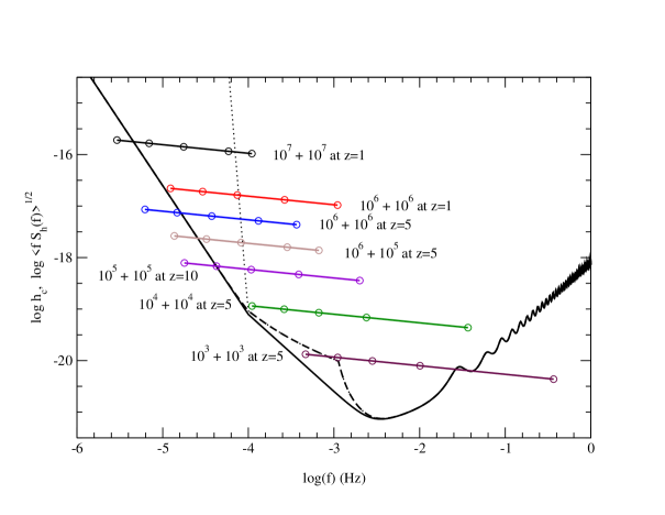
Figure 1: Characteristic strain $h_{c}$ evolution curves for several MBH binaries (masses given in ${\rm M}_{\odot}$) at various redshifts.

Figure 1 shows the evolution of inspiralling MBH binaries at various redshifts relative to LISA’s sensitivity. The thick solid line shows the baseline design sensitivity as can be obtained from the LISA Sensitivity Curve Generator [14] with an extension as $\sqrt{S_{h}(f)}\propto f^{-2}$ to frequencies below $10^{-4}$Hz based on the optimistic assumption of white acceleration noise. The dotted line represents a pessimistic scenario with a nearly vertical ($\sqrt{S_{h}(f)}\propto f^{-20}$) cut-off in sensitivity below $10^{-4}$Hz. The thick dashed line shows the expected confusion noise due to galactic binaries using the expressions in Barack and Cutler [15], which are compiled from [16, 17]. Starting at the low frequency end, the symbols on each binary evolution track denote the system at 10 years, 1 year, 1 month, 1 day before the dynamical merger, and at the onset of merger. The merger itself, as with the subsequent ringdown, produces radiation at higher frequencies.

The signal can be said to come into band when $h_{c}(f)\geq\langle fS_{h}(f)\rangle^{1/2}$. Even for the very pessimistic low frequency scenario (dotted line in figure 1), all of these systems should be detectable by LISA since they have characteristic strains $h_{c}$ significantly above the sensitivity curve. As can be seen in equation (1), the height of $h_{c}$ above the sensitivity curve provides an indication of the signal-to-noise ratio. However, to extract the binary parameters, and in particular the luminosity distance, the source must be observed by LISA over an extended period of time. For many sources, particularly those at higher $z$, this requires good sensitivity below $10^{-4}$Hz.

3 Parameter Estimation

LISA is not a pointed instrument, but rather an all-sky monitor with a predominantly quadrupolar antenna pattern. The orbital motion of LISA around the sun and the yearly rotation of the spacecraft constellation around the normal to the detector plane (which is tilted by $60^{\circ}$ with respect to the ecliptic) induce modulations of the incident gravitational waveforms that encode the source’s sky position and orientation. LISA measures both polarization components of all incident gravitational waves simultaneously, so its astronomical data will consist of essentially two time series. All the physical properties of a source, including its position and distance, must be extracted from these data streams.

This extraction process is complicated by the fact that the source parameters are entangled. For an MBH binary, the redshifted component masses, $(1+z)m_{1}$ and $(1+z)m_{2}$, can be measured by tracking the phase of the inspiral waveforms and matching the results to templates. The overall amplitudes of the gravitational waves depend on the luminosity distance $D(z)$, the chirp mass ${\cal M\,}$, and the orientation and sky position of the binary. Significant motion-induced modulations of the gravitational waveforms are needed to determine the latter two parameters well. Good observations, particularly those allowing the redshift $z$ to be extracted along with the masses, thus require the binaries to be within the band of sensitivity for a significant fraction of LISA’s yearly orbit.

Cutler [18] produced the first detailed analysis of how precisely source parameters may be estimated from LISA observations. Hughes [19] expanded on this work, providing detailed estimates of LISA’s precision in determining MBH binary positions and distances with the assumption of poor low frequency performance. Hughes and Holz [20] considered the problem of how to apply LISA observations of MBH binary systems in cosmological studies. Specifically comparing the effect of a cutoff in LISA sensitivity at $10^{-4}\mathrm{Hz}$ with that of a lower cutoff at $3\times 10^{-5}\mathrm{Hz}$, they found that the lowered cutoff provides a factor of ten improvement in distance measurement precision for an MBH binary with $m_{1}=m_{2}=10^{6}M_{\odot}$. Based on their studies Hughes and Holz proposed a rule-of-thumb, that a good measurement of source orientation and, by association, distance requires that LISA moves through one radian of its orbit, corresponding to approximately two months of observation in band.

These studies did not take into account the imprint of spin-induced precession of the orbital plane on the waveforms. Vecchio [21] recently showed that consideration of these precession effects in the data analysis can dramatically improve LISA’s parameter estimates. Rather than imposing a low frequency cutoff, he assumed that LISA observes the entire final year of the MBH binary inspiral. For two inspiralling, rapidly rotating $10^{6}M_{\odot}$ MBHs at $z=1$, Vecchio finds that the luminosity distances can typically be estimated to within $\sim 1\%$ and the masses to within $\sim 0.01\%$, while the location of the source on the sky is typically determined within an area of about a square degree. This requires the signal to be visible to LISA for $\sim 6$ months; longer observation times provide only marginal improvements in the accuracy of these parameters [22]. Below we will apply this 6 month criterion as a tool to estimate the science reach implied by various LISA sensitivity curves.

4 Low frequency sensitivity for LISA

In figure 1 we provided two sensitivity curves, representing potential realizations of LISA’s low frequency strain noise power spectrum $S_{h}(f)$. Here we consider several other plausible low frequency sensitivity realizations.

The “baseline” sensitivity curve in figure 1 should be considered extremely optimistic because it makes no allowance for likely additional sources of acceleration noise which enter at low frequencies. Specifically including some of these effects, Bender [23] has proposed a more realistic sensitivity curve which might be expected without very costly enhancements of the baseline design. His curve extends as $\sqrt{S_{h}(f)}\propto f^{-2.5}$ from $10^{-4}\mathrm{Hz}$ down to $10^{-5}\mathrm{Hz}$, and then as $\sqrt{S_{h}(f)}\propto f^{-3}$ out to $3\times 10^{-6}\mathrm{Hz}$. We call this case “Bender”, adding, in this and all cases, an extension $\sqrt{S_{h}(f)}\propto f^{-6}$ below $3\times 10^{-6}\mathrm{Hz}$. This curve just meets a proposed LISA science requirement at $10^{-5}\mathrm{Hz}$ [24]. For comparison, we consider a curve, “Relaxed”, which might correspond to a more relaxed requirement extending out directly as $\sqrt{S_{h}(f)}\propto f^{-3.5}$. The strongly pessimistic extension with a noise “Wall” below $10^{-4}$ is similar to the low frequency sensitivity considered in [19]. Because the baseline design is not guaranteed to be realized even above $10^{-4}\mathrm{Hz}$, we also consider a case with relaxed sensitivity across the band. This case corresponds to a conceivably “de-scoped” version of LISA, degraded by a factor of ten from the Relaxed case.

5 Science Reach for MBH Binary Inspirals

Uncovering the merger history of MBHs in the evolving universe using gravitational waves requires that LISA observations provide the masses, sky positions, and redshifts of these sources. Quantifying this discovery space requires that we specify a threshold criterion for a sufficently informative observation. Based on the discussion in section 3, we apply the rule-of-thumb that LISA must observe the source for $t_{\rm obs}=6$ months in band. Otherwise, recent studies of parameter estimation accuracy suggest that we should not expect a good measurement of the luminosity distance and position on the sky. It should be noted that incomplete information, such as the redshifted chirp mass $(1+z){\cal M\,}$, may nonetheless be determinable for systems which fail our criterion.

We now proceed to map this discovery space parametrized in terms of the chirp mass ${\cal M\,}$and the redshift $z$. At a fixed time $t_{\rm obs}$ prior to coalescence, the system’s signal is characterized by frequency $f(t_{\rm obs},{\cal M\,},z)$ given by equation (4). We also need the characteristic strain at this frequency, at time $t_{\rm obs}$ before coalescence. To obtain this, we eliminate ${\cal M\,}$in equation (3); this gives

$$h_{c}(t_{\rm obs},z,f)=2.8\times 10^{-17}\left(\frac{D_{L}(z)}{1\;{\rm Gpc}}\right)^{-1}\left(\frac{t_{\rm obs}}{6\;{\rm mos.}}\right)^{-1/2}\left(\frac{f}{10^{-4}\mathrm{Hz}}\right)^{-3/2}.$$ (5)

If, at $t_{\rm obs}=6$ months, this strain is larger than LISA’s annually averaged unitless strain noise at this frequency, i.e. above the sensitivity curve $h_{c}>\langle fS_{h}(f)\rangle^{1/2}$, then a system of the specified chirp mass and redshift will be identified as being “in band” for at least 6 months, thus meeting the criterion for a minimum adequate observation.

Plotting the values given by equations (3) and (4) with candidate realizations of LISA’s unitless strain noise $\langle fS_{h}(f)\rangle^{1/2}$ allows us to make a map, shown in figure 2, of which systems are accessible.

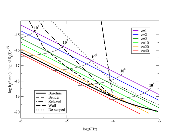
Figure 2: Sources which can be adequately observed by LISA with the various low frequency sensitivity curves discussed in Section 4. Potential sources are labeled by redshift $z$ and chirp mass ${\cal M\,}$ (in ${\rm M}_{\odot}$). The range of sources falling above a particular sensitivity curve would be observable for a minimum of six months by the corresponding realization of LISA. The sensitivity curves shown represent a combination of instrumental noise and confusion noise from the astrophysical WD-WD background.

The sensitivity curves shown represent the instrumental sensitivity models described in section 4 added to a model of binary white dwarf noise given in [15]. The colored lines depict MBH binary systems at $t_{\rm obs}=6$ months prior to coalescence at specified redshifts ranging from $z=1$ to $z=40$. These are crossed by a set of thin solid dark curves denoting the chirp masses ${\cal M\,}$of systems observed at frequency $f$ at time $t_{\rm obs}=6$ months. Together these form a grid representing the variety of potentially observable astrophysical systems. Regions of the grid which lie above a particular sensitivity curve correspond to systems which can be observed by that version of LISA for at least 6 months.

This figure indicates which systems we can expect the various versions of LISA to observe effectively at large redshift. In particular, it suggests that, for large redshift observations, LISA will likely have a “sweet spot” near $10^{-4}\mathrm{Hz}$, and will be most sensitive to systems of chirp mass around ${\cal M\,}\sim 10^{4}$-$10^{5}{\rm M}_{\odot}$. If the baseline sensitivity is achieved at this frequency, then the 6 month criterion suggests that LISA may be able to observe such systems out to $z\sim 20$. Since the slope of the constant redshift curves is precisely the same as the slope of the baseline sensitivity curve dominated by white acceleration noise, this region can be extended for as far as the baseline sensitivity curve can be preserved, allowing larger systems to be observed to the same redshift.

The ability to observe high-redshift systems with mass near ${\cal M\,}\sim 10^{6}{\rm M}_{\odot}$ will be determined by the sensitivity near $10^{-5}\mathrm{Hz}$. The difference between Bender’s proposal and the relaxed sensitivity curve is significant in this range and implies a change by about a factor of three in the redshift to which LISA will be able to see. Bender’s sensitivity allows observation to a redshift of $z\sim 10$. A noise wall above $3\times 10^{5}\mathrm{Hz}$ might completely obscure the late inspirals of these systems. Likewise, observation of any systems beyond $z=1$ with masses larger than ${\cal M\,}\sim 10^{7}{\rm M}_{\odot}$ would require fair sensitivity below $10^{-5}\mathrm{Hz}$. De-scoping LISA as described in Section 4 would constrain observations to lower redshifts, $z<4$ for ${\cal M\,}\sim 10^{4}{\rm M}_{\odot}-10^{5}{\rm M}_{\odot}$ and $z<1$ for ${\cal M\,}\sim 10^{6}{\rm M}_{\odot}$.

6 Discussion

We have considered the observability of MBH binary systems at redshifts $z>1$ by LISA for several possible low frequency sensitivities, $f<10^{-4}$Hz. We distinguish between detection of the binary, in which the LISA data stream would contain a signal from these sources at good SNR (cf. figure 1) and observation, in which the binary parameters such as component masses, spins, luminosity distance and sky position can be extracted accurately. Assuming that successful parameter extraction relies on using the motion-induced modulations of the gravitational waveforms, we applied the rule that an MBH binary system must be monitored by LISA for 6 months in band for a good observation [22]. Figure 2 shows that good sensitivity, given by the Bender curve, at $f\sim 10^{-5}$Hz will allow LISA to observe MBH binaries with ${\cal M\,}\sim 10^{6}{\rm M}_{\odot}$ out to $z\sim 10$. Lower mass systems, ${\cal M\,}\sim 10^{4}{\rm M}_{\odot}-10^{5}{\rm M}_{\odot}$, could be observed out $z\sim 20$ if the sensitivity is near the baseline design at $f\sim 10^{-4}$Hz.

We have considered only the lowest order quadrupolar waves from MBH binary inspirals. Including higher order multipole components [25] could improve the parameter extraction, lessening the amount of time needed for a good observation. Such a relaxation of the 6 month-in-band rule would allow LISA to see MBH binaries to even higher redshifts for the low frequency sensitivities discussed here. For example, using the Relaxed sensitivity curve, equation (5) shows that LISA could observe ${\cal M\,}\sim 10^{6}{\rm M}_{\odot}$ binaries out to $z\sim 8$ for a six-week-in band observation, should such sources exist. These considerations deserve further study as the specification of LISA’s design is completed. Similarly, if monitoring only the final radiation burst is found to allow an adequate estimation of the system parameters, or if incomplete observations that only allow determination of some parameters (such as $(1+z){\cal M\,}$, for example) are considered adequate, then many more systems could be deemed observable. We are currently investigating these issues.

Good low frequency sensitivity for LISA has considerable astrophysical value. Knowledge of the binary parameters will reveal the merger history of MBHs and, by implication, their host structures as the universe evolves. Current models for MBH growth and cosmic structure formation yield different predictions for the rate of MBH binary mergers. LISA observations of these systems will provide direct dynamical information about the number of events at different redshifts. Comparing these data with model predictions will discriminate between different scenarios (e.g., [1, 3, 4, 5]), shedding light on the relative importance of mechanisms such as accretion and mergers for MBH growth and structure formation.

References

References

- [1] A. Sesana, F. Haardt, P. Madau, and M. Volonteri, (2004).
- [2] A. Sesana, these proceedings, 2004.
- [3] J. S. B. Wyithe and A. Loeb, Astrophys. J. 590, 691 (2003).
- [4] M. G. Haehnelt, Class. Quant. Grav. 20, S31 (2003).
- [5] M. Haehnelt, in Carnegie Observatories Astrophysics Series, Vol. 1: Coevolution of Black Holes and Galaxies, edited by L. C. Ho (Cambridge University Press, Cambridge, 2004).
- [6] L. Blanchet, Living Rev. Rel. 5, 3 (2002).
- [7] B. Bruegmann, W. Tichy, and N. Jansen, Phys. Rev. Lett. 92, 211101 (2004).
- [8] E. W. Leaver, Proc. Roy. Soc. Lond. A402, 285 (1985).
- [9] F. Echeverria, Phys. Rev. D40, 3194 (1989).
- [10] E. E. Flanagan and S. A. Hughes, Phys. Rev. D57, 4535 (1998).
- [11] D. N. Spergel et al., Astrophys. J. Suppl. 148, 175 (2003).
- [12] S. A. Hughes, Class. Quant. Grav. 18, 4067 (2001).
- [13] L. Blanchet, G. Faye, B. R. Iyer, and B. Joguet, Phys. Rev. D65, 061501 (2002).
- [14] S. Larson, http://www.srl.caltech.edu/ shane/sensitivity/, 2003.
- [15] L. Barack and C. Cutler, Phys. Rev. D69, 082005 (2004).
- [16] A. J. Farmer and E. S. Phinney, Mon. Not. Roy. Astron. Soc. 346, 1197 (2003).
- [17] G. Nelemans, L. R. Yungelson, and S. F. Portegies Zwart, Astron. and Astrophys. 375, 890 (2001).
- [18] C. Cutler, Phys. Rev. D57, 7089 (1998).
- [19] S. A. Hughes, Mon. Not. Roy. Astron. Soc. 331, 805 (2002).
- [20] S. A. Hughes and D. E. Holz, Class. Quant. Grav. 20, S65 (2003).
- [21] A. Vecchio, Phys. Rev. D70, 042001 (2004).
- [22] A. Vecchio, these proceedings, 2004.
- [23] P. L. Bender, Class. Quant. Grav. 20, S301 (2003).
- [24] T. Prince, LISA Science Requirements, LISATools project archive, 2001.
- [25] R. W. Hellings and T. A. Moore, Class. Quant. Grav. 20, S181 (2003).