The iron $K_{\alpha}$-line as a tool for an evaluation of black hole parameters

Abstract

Recent X-ray observations of microquasars and Seyfert galaxies reveal broad emission lines in their spectra, which can arise in the innermost parts of accretion disks. Simulations indicate that at low inclination angle the line is measured by a distant observer as characteristic two-peak profile. However, at high inclination angles ($>85^{0}$) two additional peaks arise. This phenomenon was discovered by Matt et al. (1993) using the Schwarzschild black hole metric to analyze such effect. They assumed that the effect is applicable to a Kerr metric far beyond the range of parameters that they exploited. We check and confirm their hypothesis about such a structure of the spectral line shape for the Kerr metric case. We use no astrophysical assumptions about the physical structure of the emission region except the assumption that the region should be narrow enough. Positions and heights of these extra peaks drastically depend on both the radial coordinate of the emitting region (annuli) and the inclination angle. It was found that these extra peaks arise due to gravitational lens effect in the strong gravitational field, namely they are formed by photons with some number of revolutions around black hole. This conclusion is based only on relativistic calculations without any assumption about physical parameters of the accretion disc like X-ray surface emissivity etc. We discuss how analysis of the iron spectral line shapes could give an information about an upper limit of magnetic field near black hole horizon.

1 SIGNATURES OF HIGHLY INCLINATED ACCRETION DISKS NEAR GBHCs AND AGNs

More than ten years ago it was predicted that profiles of lines emitted by AGNs and X-ray binary systems could have an asymmetric double-peaked shape (e.g. Chen et al. (1989); Fabian et al. (1989); Matt, Perola & Stella (1993)). Generation of the broad $K_{\alpha}$ fluorescence lines as a result of irradiation of a cold accretion disk was discussed by many authors (see, for example, Matt et al (1992a, b); Matt & Perola (1992); Matt et al. (1993); Bao (1993); Martocchia at al. (2002b) and references therein). Popovic et al. (2001, 2003) discussed influence of microlensing on the distortion of spectral lines including Fe $K_{\alpha}$ line, that can be significant in some cases. Zakharov et al. (2003c) showed that the optical depth for microlensing could be significant for cosmological distributions of microlenses. Recent X-ray observations of Seyfert galaxies, microquasars and binary systems (Fabian et al. (1995); Tanaka et al. (1995); Nandra et al. (1997a, b); Malizia et al. (1997); Sambruna et al. (1998); Yaqoob et al. (2001); Ogle et al. (2000); Miller et al. (2002) and references therein) confirm these considerations in general and reveal broad emission lines in their spectra with characteristic two-peak profiles. A comprehensive review by Fabian et al. (2000) summarizes the detailed discussion of theoretical aspects of possible scenarios for generation of broad iron lines in AGNs. These lines are assumed to arise in the innermost parts of the accretion disk, where the effects of General Relativity (GR) must be taken into account, otherwise it appears very difficult to find a natural explanation for observed line profile.

Numerical simulations of the line structure are be found in a number of papers Bao (1993); Kojima (1991); Laor (1991); Bao & Stuchlik (1992); Bao, Hadrava & Ostgaard (1994); Bromley et al. (1997); Fanton et al. (1997); Pariev & Bromley (1997, 1998); Pariev et al. (2001); Ruszkowski M. (2000); Ma (2002). They indicate that the accretion disks in Seyfert galaxies are usually observed at the inclination angle $\theta$ close to $30^{0}$ or less. This occurs because according to the Seyfert galaxy models, an opaque dusty torque surrounds the accretion disk which does not allow us to observe the disk at larger inclination angles.

However, at inclination angles $\theta>80^{0}$, new observational manifestations of GR could arise. (Matt, Perola & Stella (1993) discovered such phenomenon for a Schwarzschild black hole, moreover the authors predicted that their results could be applicable to a Kerr black hole over the range of parameters exploited). The authors mentioned that this problem was not analyzed in detail for a Kerr metric case and it would be necessary to investigate this case. Below we do not use a specific model on surface emissivity of accretion (we only assume that the emitting region is narrow enough). But general statements (which will be described below) can be generalized to a wide disk case without any problem. Therefore, in this paper we check and confirm their hypothesis for the Kerr metric case and for a Schwarzschild black hole using other assumptions about surface emissivity of accretion disks. In principle, such a phenomenon could be observed in microquasars and X-ray binary systems where there are neutron stars and black holes with stellar masses.

1.1 Numerical methods

We used an approach discussed in detail in papers Zakharov (1991, 1993, 1994); Zakharov & Repin (1999, 2002a, 2001, 2002b, 2002c, 2002d, 2003a, 2003d, 2003e, 2004a, 2003a, 2003b, 2003c); Zakharov et al. (2003a). The approach was used in particular to simulate spectral line shapes. For example, Zakharov et al. (2003a) used this approach to simulate the influence of a magnetic field on spectral line profiles. This approach is based on results of a qualitative analysis (which was done by for different types of geodesics near a Kerr black hole Zakharov (1986, 1989)). The equations of photon motion in the Kerr metric are reduced to the following system of ordinary differential equations in dimensionless Boyer – Lindquist coordinates Zakharov (1991, 1994):

$$\frac{dt}{d\sigma} = -a\left(a\sin^{2}\theta-\xi\right)+\frac{r^{2}+a^{2}}{\Delta}\left(r^{2}+a^{2}-\xi a\right),$$ (1)

$$\frac{dr}{d\sigma} = r_{1},$$ (2)

$$\frac{dr_{1}}{d\sigma} = 2r^{3}+\left(a^{2}-\xi^{2}-\eta\right)r+\left(a-\xi\right)^{2}+\eta,$$ (3)

$$\frac{d\theta}{d\sigma} = \theta_{1},$$ (4)

$$\frac{d\theta_{1}}{d\sigma} = \cos\theta\left(\frac{\xi^{2}}{\sin^{3}\theta}-a^{2}\sin\theta\right),$$ (5)

$$\frac{d\phi}{d\sigma} = -\left(a-\frac{\xi}{\sin^{2}\theta}\right)+\frac{a}{\Delta}\left(r^{2}+a^{2}-\xi a\right),$$ (6)

where $\Delta=r^{2}-2r+a^{2}$; $\eta=Q/M^{2}E^{2}$ and $\xi=L_{z}/ME$ are the Chandrasekhar constants Chandrasekhar (1983) which are derived from the initial conditions of the emitted quantum in the disk plane. The system (1)-(6) has two first integrals

$$\epsilon_{1} \equiv r_{1}^{2}-r^{4}-\left(a^{2}-\xi^{2}-\eta\right)r^{2}-2\left[\left(a-\xi\right)^{2}+\eta\right]r+a^{2}\eta=0,$$ (7)

$$\epsilon_{2} \equiv \theta_{1}^{2}-\eta-\cos^{2}\theta\left(a^{2}-\frac{\xi^{2}}{\sin^{2}\theta}\right)=0,$$ (8)

which can be used for the accuracy control of computation.

Solving Eqs. (1)–(6) for monochromatic quanta emitted by a ring we can calculate a spectral line shape $I_{\nu}(r,\theta)$ which is registered by a distant observer at inclination angle $\theta$.

1.2 Disk model

To simulate the structure of the emitted line it is necessary first to choose a model for the emissivity of an accretion disk. We exploit two different models, namely we consider a narrow and thin disk moving in the equatorial plane near a Kerr black hole as the first model and as we analyze the inner wide part of an accretion disk with a temperature distribution which is chosen according to the Shakura & Sunyaev (1973); Lipunova & Shakura (2002) with fixed inner and outer radii $r_{i}$ and $r_{o}$ as the second model. Usually a power law is used for wide disk emissivity (see, for example, Laor (1991); Martocchia & Matt (1996); Martocchia et al. (2000, 2002a)). However, other models for emissivity can not be excluded for such a wide class of accreting black holes, therefore, to demonstrate how another emissivity law could change line profiles we investigate such a emissivity law.

First, we assume that the source of the emitting quanta is a narrow thin disk rotating in the equatorial plane of a Kerr black hole. We also assume that the disk is opaque to radiation, so that a distant observer situated on one disk side cannot measure the quanta emitted from its other side.

For second case of the Shakura – Sunyaev disk model, we assume that the local emissivity is proportional to the surface element and and $T^{4}$, where $T$ is a local temperature. The emission intensity of the ring is proportional to its area. The area of the emitting ring (width $dr$) differs in the Kerr metric from its classical expression $dS=2\pi rdr$ and should be replaced with

$$dS=\frac{2\pi\left(r^{2}+a^{2}\right)}{\displaystyle\sqrt{r^{2}-rr_{g}+a^{2}\phantom{1}}}\,dr.$$ (9)

For simulation purposes we assume that the emitting region lies entirely in the innermost region of the $\alpha$-disk (zone $a$) from $r_{out}=10\,r_{g}$ to $r_{in}=3\,r_{g}$ and the emission is monochromatic in the co-moving frame. The frequency of this emission set as unity by convention.

1.3 Simulation results

Figure 1: Line profiles for high inclination angles, $\theta>85^{0}$, due to gravitational lens effects in the strong gravitational field approach. The Kerr (rotation) parameter was chosen as $a=0.9981$. The radii decrease from top to bottom, the inclination angles increase from left to right; their values are shown in each panel along with the number of quanta included in the spectrum.

Spectral line profiles of a narrow ring observed at large inclination angles $\theta>85^{0}$ and different radii $r$ are shown in Fig. 1 (a Kerr metric generalization of Fig. 1 from Matt, Perola & Stella (1993) which was drawn using calculations for the Schwarzschild case). The ring is assumed to move in the equatorial plane of a Kerr black hole with an almost extreme rotation parameter $a=0.9981$. The inclination angle increases from left to right and the radial coordinate from bottom to top. The figure indicates that there are practically no new specific features of profiles, thus, the line profile remains one-peaked with a maximum close to $1.6\,E_{lab}$ and a very long red wing without any significant details.

For the lowest radii there are no signatures of multiple peaks of spectral line shapes even for high inclination angles (the bottom row in Fig. 1 which corresponds to $r=0.8\,r_{g}$).

Increasing the radius to $r=1.2\,r_{g}$, an additional blue peak arises in the vicinity of the blue maximum at the highest inclination angle $\theta=89^{0}$. The red maximum is so small that no details can be distinguished in its structure. At lower inclination angles $\theta\leq 88^{0}$ the blue maximum also has no details and the entire line profile remains essentially one-peaked.

For $r=3\,r_{g}$ additional details in the blue peak appear for $\theta\geq 85^{0}$. Thus, for $\theta=85^{0}$ we have a fairly clear bump, at $\theta=88^{0}$ it changes into a small complementary maximum and for $\theta=89^{0}$ this maximum becomes well-distinguished. Its position in the last case differs significantly from the main maximum: $E_{3}=1.12\,E_{lab}$, $E_{4}=1.34\,E_{lab}$.

When further increasing the radius the red maximum also bifurcates. This effect becomes visible for $r=5\,r_{g}$ and $\theta\geq 88^{0}$. Thus, for $\theta=85^{0}$ we have only a faintly discernible (feebly marked) bump, but for $\theta=88^{0}$ both complementary maxima (red and blue) arise. For $\theta=89^{0}$ we have already four maxima in the line profile: $E_{1}=0.63\,E_{lab}$, $E_{2}=0.66\,E_{lab}$, $E_{3}=1.07\,E_{lab}$, $E_{4}=1.28\,E_{lab}$. Note that the splitting for the blue and red maxima is not equal, moreover, $E_{4}-E_{3}\approx 7\,\left(E_{2}-E_{1}\right)$.

For $r=10\,r_{g}$ the profile becomes more narrow, but the complementary peaks appear very distinctive. We have a four-peak structure for $\theta\geq 88^{0}$. It is interesting to note that for $\theta=89^{0}$ the energy of the blue complementary peak is close to its laboratory value.

Note that the effect almost disappears when the radial coordinate becomes less than $r_{g}$, i.e. for the orbits which could exist only near a Kerr black hole.

Figure 2: Details of a hot spot line profile for the most distinctive case with $r=10\,r_{g}$ and $a=0.9981$ (see the top row of Fig. 1). The images of all orders are counted. The left panel includes all the quanta, registered at infinity with $\theta>89^{0}$. The right panel includes the quanta with $\theta>89.5^{0}$.

Figure 3: Details of the line structure for an $\alpha$-disk in the Schwarzschild metric with outer and inner edges of emitting region equal to $r_{out}=10\,r_{g}$ and $r_{in}=3\,r_{g}$, respectively. The left panel includes all the quanta, registered at infinity with $\theta>89^{0}$. The right panel includes the quanta with $\theta>89.5^{0}$.

Fig. 2 demonstrates the details of the spectrum presented in the top row in Fig. 1. Thus, the left panel includes all the quanta emitted by a hot spot at $r=10\,r_{g}$ with $\theta>89^{0}$ at infinity (the mean value could be counted as $85.5^{0}$ if the quanta distribution would be uniform there) but with much higher resolution than in Fig. 1. The spectrum has four narrow distinctive maxima separated by lower emission intervals. In the right panel, which includes all the quanta with $\theta>85.5^{0}$, the right complementary maxima is even higher than the main one. The blue complementary maxima still remains lower than its main counterpart, but it increases rapidly its intensity with increasing inclination angle. It follows immediately from the comparison of the left and right panels. The ”oscillation behavior” of the line profile between the maxima has a pure statistical origin and is not caused by the physics involved.

As an illustration, a spectrum of an entire accretion disk at high inclination angles in the Schwarzschild metric is shown in Fig. 3. (In reality we have calculated geodesics for the quanta trajectories in the Schwarzschild metric using the same Eqs. (1)–(6) as for a Kerr metric, but assuming there $a=0.01$.) The emitting region (from 3 to $10\,r_{g}$) lies as a whole in the innermost region of the $\alpha$-disk (the detailed description of this model was given by Shakura & Sunyaev (1973); Lipunova & Shakura (2002)).

As follows from Fig. 3, the blue peak may consist of the two components, whereas the red one remains unresolved.

1.4 Discussion and conclusions

The complicated structure of the line profile at large inclination angles is explained by the multiple images of some pieces of the hot ring. We point out that the result was obtained in the framework of GR without any extra physical and astrophysical assumptions about the character of the radiation etc. For a Kerr black hole we assume only that the radiating ring is circular and narrow.

The problem of multiple images in the accretion disks and extra peaks was first considered by Matt, Perola & Stella (1993) (see also Bao (1993); Bao & Stuchlik (1992); Bao, Hadrava & Ostgaard (1994); Bao et al. (1996)). Using numerical simulations Matt, Perola & Stella (1993) proved the statement for the Schwarzschild metric and suggested that the phenomenon is applicable to a Kerr metric over the range of parameters that the authors have analyzed. They noted also that it is necessary to perform detailed calculations to confirm their hypothesis. We verified and confirmed their conjecture without any assumptions about a specific distribution of surface emissivity or accretion disk model (see Fig. 1,2).

We confirmed also their conclusion that extra peaks are generated by photons which are emitted by the far side of the disk, therefore we have a manifestation of gravitational lensing in the strong gravitational field approach for GR.

Some possibilities to observe considered features of spectral line profiles were considered by Matt, Perola & Stella (1993); Bao (1993). The authors argued that there are non-negligible chances to observe such phenomenon in some AGNs and X-ray binary systems. For example, Bao (1993) suggested that NGC 6814 could be a candidate to demonstrate such a phenomenon (but Madejski et al. (1993) found that the peculiar properties of NGC6814 are caused by a cataclysmic variable like an AM Herculis System).

However, it is clear that in general the probability to observe objects where one could find such features of spectral lines is small. Moreover, even if the inclination angle is very close to $90^{0}$, the thickness of the disk ( shield or a torus around an accretion disk) may not allow us to look at the inner part of accretion disk. Here, discuss astrophysical situations when the the inclination angle of the accretion disk is high enough.

About 1% of all AGN or microquasar systems could have an inclination angle of the accretion disk $>89^{0}$. For example, Kormendy et al. (1996) found that NGC3115 has a very high inclination angle about of $81^{0}$ (Kormendy & Richstone (1992) discovered a massive dark object $M\sim 10^{9}M_{\odot}$(probably a massive black hole) in NGC3115). Perhaps we have a much higher probability to observe such a phenomenon in X-ray binary systems where black holes with stellar masses could be. Taking into account the precession which is actually observed for some X-ray binary systems (for example, there is a significant precession of the accretion disk for the SS433 binary system Cherepashchuk (2002), moreover since the inclination of the orbital plane is high ($i\sim 79^{0}$ for this object) sometimes we may observe almost edge-on accretion disks of such objects. Observations indicated that there is a strong evidence that the optically bright accretion disk in SS433 is in a supercritical regime of accretion. The first description of a supercritical accretion disk was given by Shakura & Sunyaev (1973). Even now such a model is discussed to explain observational data for SS433 Cherepashchuk (2002). We used the temperature distribution from the Shakura – Sunyaev model Shakura & Sunyaev (1973); Lipunova & Shakura (2002) for the inner part of accretion disk to simulate shapes of lines which could be emitted from this region (Fig. 3). Therefore, we should conclude that the properties of spectral line shapes discovered by Matt, Perola & Stella (1993) are confirmed also for such emissivity (temperature) distributions which correspond to the Shakura – Sunyaev model.

Thus, such properties of spectral line shapes are robust enough with respect to wide variations of rotational parameters of black holes and the surface emissivity of accretion disks as it was predicted by Matt, Perola & Stella (1993). So, their conjecture was confirmed not only for the Kerr black hole case but also for other dependences of surface emissivity of the accretion disk. A detailed description of the analysis was given by Zakharov & Repin (2003a).

2 MAGNETIC FIELDS IN AGNs AND MICROQUASARS

Magnetic fields play a key role in dynamics of accretion discs and jet formation. Bisnovatyi-Kogan & Ruzmaikin (1974, 1976) considered a scenario to generate superstrong magnetic fields near black holes. According to their results magnetic fields near the marginally stable orbit could be about $H\sim 10^{10}-10^{11}$ G. Kardashev (1995, 2001) has shown that the strength of the magnetic fields near supermassive black holes can reach the values $H_{max}\approx 2.3\cdot 10^{10}M_{9}^{-1}$ G due to the virial theorem, and considered a generation of synchrotron radiation, acceleration of $e^{+/-}$ pairs and cosmic rays in magnetospheres of supermassive black holes at such high fields. It is magnetic field, which plays a key role in these models. Below, based on the analysis of iron $K_{\alpha}$ line profile in the presence of a strong magnetic field, we describe how to detect the field itself or at least obtain an upper limit of the magnetic field.

General status of black holes is described in a number of papers (see, e.g. Zakharov (2000) and references therein). Since the matter motions indicate very high rotational velocities, one can assume the $K_{\alpha}$ line emission arises in the inner regions of accretion discs at distances $\sim(1\div 3)~{}r_{g}$ from the black holes. Let us recall that the innermost stable circular for non-rotational black hole (which has the Schwarzschild metric) is located at the distance $3\,r_{g}$ from the black hole singularity. Therefore, a rotation of black hole could be the most essential factor.

Wide spectral lines are considered to be formed by radiation emitted in the vicinity of black holes. If there are strong magnetic fields near black holes these lines are split by the field into several components. This phenomenon is discussed below. Such lines have been found in microquasars, GRBs and other similar objects (Mirabel & Rodriguez, 2002; Miller et al., 2002).

To obtain an estimation of the magnetic field we simulate the formation of the line profile for different values of magnetic field. As a result we find the minimal $B$ value at which the distortion of the line profile becomes significant. Here we use an approach, which is based on numerical simulations of trajectories of the photons emitted by a hot ring moving along a circular geodesics near black hole, described earlier by Zakharov (1993, 1994); Zakharov & Repin (1999); Zakharov (1995).

2.1 Influence of a magnetic field on the distortion of the iron $K_{\alpha}$ line profile

Here we consider the influence of a magnetic field on the iron $K_{\alpha}$ line profile and show how one can determine the value of the magnetic field strength or at least an upper limit.

The profile of a monochromatic line (Zakharov & Repin, 1999, 2002a) depends on the angular momentum of a black hole, the position angle between the black hole axis and the distant observer position, the value of the radial coordinate if the emitting region represents an infinitesimal ring (or two radial coordinates for outer and inner bounds of a wide disc). The influence of accretion disc model on the profile of spectral line was discussed by (Zakharov & Repin, 2003b).

We assume that the emitting region is located in the area of a strong quasi-static magnetic field. This field causes line splitting due to the standard Zeeman effect. There are three characteristic frequencies of the split line that arise in the emission. The energy of central component $E_{0}$ remains unchanged, whereas two extra components are shifted by $\pm\mu_{B}H$, where $\mu_{B}=\dfrac{e\hbar}{2m_{\rm e}c}=9.273\cdot 10^{-21}$ erg/G is the Bohr magneton. Therefore, in the presence of a magnetic field we have three energy levels: $E_{0}-\mu_{B}H,~{}E_{0}$ and $E_{0}+\mu_{B}H$. For the iron $K_{\alpha}$ line they are as follows: $E_{0}=6.4-0.58\dfrac{H}{10^{11}\,{\rm G}}$ keV, $E_{0}=6.4$ keV and $E_{0}=6.4+0.58\dfrac{H}{10^{11}\,{\rm G}}$ keV.

Let us discuss how the line profile changes when photons are emitted in the co-moving frame with energy $E_{0}(1+\epsilon)$, but not with $E_{0}$. In that case the line profile can be obtained from the original one by $1+\epsilon$ times stretching along the x-axis which counts the energy. The component with $E_{0}(1-\epsilon)$ energy should be $(1-\epsilon)$ times stretched, respectively. The intensities of different Zeeman components are approximately equal (Fock, 1978). A composite line profile can be found by summation the initial line with energy $E_{0}$ and two other profiles, obtained by stretching this line along the $x$-axis in $(1+\epsilon)$ and $(1-\epsilon)$ times correspondingly. The line intensity depends on the direction of the quantum escape with respect to the direction of the magnetic field (Berestetskii et al., 1982). However, we neglect this weak dependence (undoubtedly, the dependence can be counted and, as a result, some details in the spectrum profile can be slightly changed, but the qualitative picture, which we discuss, remains unchanged).

Figure 4: Profile of monochromatic spectral line, emitted by $\alpha$-disc in Schwarzschild metric for $r_{out}=10\,r_{g}$, $r_{in}=3\,r_{g}$ and inclination angles $\theta=60^{\circ}$ (top panel) and $\theta=50^{\circ}$ (bottom panel) with zero value of magnetic field. The line profile is represented as it is registered by a distant observer.

Figure 5: Distortions of the line profile from the top panel in Fig. 4, arising due to a quasi-static magnetic field existing in the disc. The Zeeman effect leads to the appearance of two extra components with the energies higher and lower than the basic one. The values of the magnetic field are shown at each panel.

Another indicator of the Zeeman effect is a significant induction of the polarization of X-ray emission: the extra lines possess a circular polarization (right and left, respectively, when they are observed along the field direction) whereas a linear polarization arises if the magnetic field is perpendicular to the line of sight.Despite of the fact that the measurements of polarization of X-ray emission have not been carried out yet, such experiments can be realized in the nearest future (Costa et al., 2001).

Figure 6: The same as in Fig. 5, but for $\theta=50^{0}$. The bottom panel on Fig. 4 demonstrates the same spectrum without magnetic field.

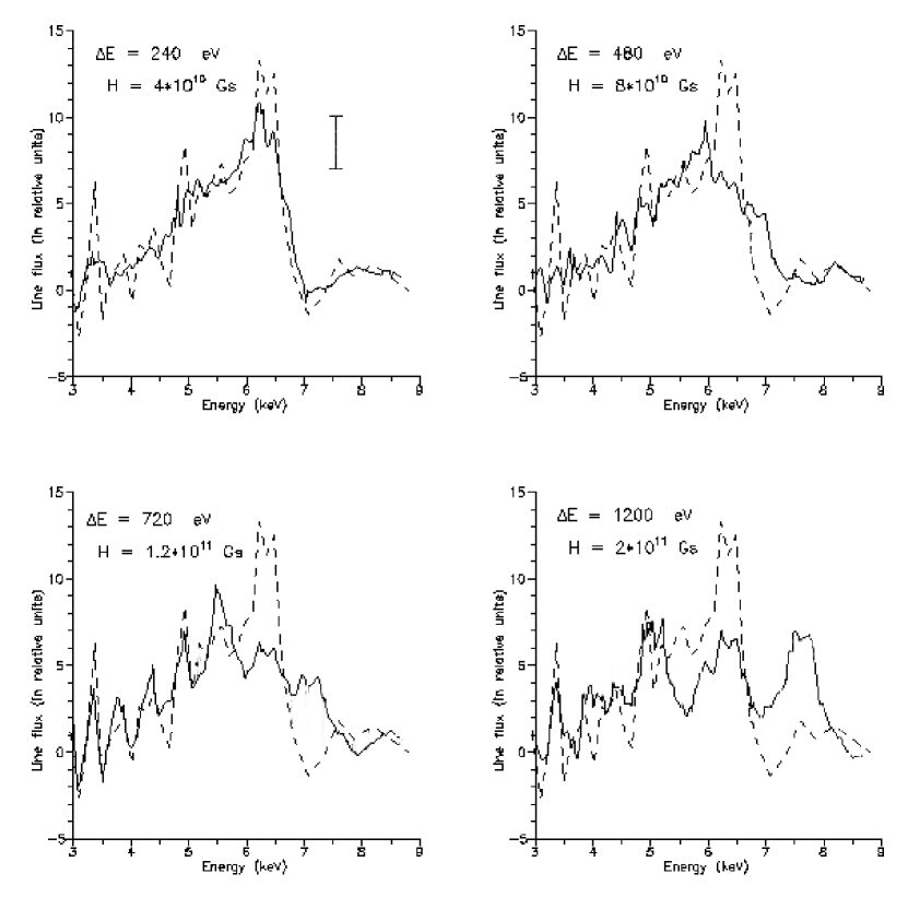
Figure 7: Influence of a magnetic field on the observational data. The dashed line represents the ASCA observations of MCG-6-30-15 (Tanaka et al., 1995). The vertical bar in the top left panel corresponds to a typical error in observation data. Solid lines show possible profiles of $K_{\alpha}$ line in a presence of a magnetic field. The field value and the appropriate Zeeman splitting are indicated in each panel.

The line profile without any magnetic field is presented in Fig. 4 for different values of disc inclination angles: $\theta=60^{0}$ and $\theta=50^{0}$ respectively. Note, that at $\theta=50^{0}$ the blue peak appears to be taller and more narrow. Figs. 5,6 present the line profiles for the same inclination angles and different values of magnetic field: $H=4\cdot 10^{10}$, $8\cdot 10^{10}$, $1.2\cdot 10^{11}$, $2\cdot 10^{11}$ G. At $H=4\cdot 10^{10}$ G the shape of spectral line does not practically differ from the one with zero magnetic field. Three components of the blue peak are so thin and narrow that they could scarcely be distinguished experimentally today. For $H<4\cdot 10^{10}$ G and $\theta=60^{0}$ the splitting of the line does not arise at all. At $\theta=50^{0}$ the splitting can still be revealed for $H=3\cdot 10^{10}$ G, but below this value ($H<3\cdot 10^{10}$ G) it also disappears. With increasing the field the splitting becomes more explicit, and at $H=8\cdot 10^{10}$ G a faint hope appears to register experimentally the complex internal structure of the blue maximum.

While further increasing the magnetic field the peak profile structure becomes apparent and can be distinctly revealed, however, the field $H=2\cdot 10^{11}$ G is rather strong, so that the classical linear expression for the Zeeman splitting

$$\Delta E=\pm\mu_{B}H$$ (10)

should be modified. Nevertheless, we use Eq.(10) for any value of the magnetic field, assuming that the qualitative picture of peak splitting remains correct, whereas for $H=2\cdot 10^{11}$ G the exact maximum positions may appear slightly different. If the Zeeman energy splitting $\Delta E$ is of the order of $E$, the line splitting due to magnetic fields is described in a more complicated way. The discussion of this phenomenon is not a point of this paper, our aim is to pay attention to the qualitative features of this effect.

Let us discuss possible influence of high magnetic fields on real observational data. We will try to estimate magnetic fields when one could find the typical features of line splitting from the analysis of the spectral line shape. Further we will choose some values of magnetic field and simulate the spectral line shapes from observational data for these values, assuming that these observational data correspond to an object with no significant magnetic fields. We will try to find signatures of the triple blue peak analyzing the simulated data when magnetic fields are rather high. Assuming that there are no essential magnetic fields (compared to $10^{10}$ G) for some chosen object (for example, for MCG 6-30-15) we could simulate the spectral line shapes for the same objects but with essential magnetic fields. Fig. 7 demonstrates a possible influence of the Zeeman effect on observational data. As an illustration we consider the observations of iron $K_{\alpha}$ line which have been carried out by ASCA for the galaxy MCG-6-30-15. They are presented in Fig. 7 in the dashed curve. Let us assume that the actual magnetic field in these data is negligible. Then we can simulate the influence of the Zeeman effect on the structure of observations and see if the simulated data (with a magnetic field) can be distinguishable within the current accuracy of the observations. The results of the simulated observation for the different values of magnetic field are shown in Fig. 7 in solid line. From these figures one can see that classical Zeeman splitting in three components, which can be revealed experimentally today, changes qualitatively the line profiles only for rather high magnetic field. Something like this structure can be detected, e.g. for $H=1.2\cdot 10^{11}$ G, but the reliable recognition of three peaks here is hardly possible.

Apparently, it would be more correct to solve the inverse problem: try to determine the magnetic field in the disc, assuming that the blue maximum is already split due to the Zeeman effect. However, this problem includes too many additional factors, which can affect on the interpretation. Thus, besides magnetic field the line width depends on the accretion disc model as well as on the structure of emitting regions. Problems of such kind may become actual with much better accuracy of observational data in comparison with their current state.

2.2 Discussion

It is evident that duplication (triplication) of a blue peak could be caused not only by the influence of a magnetic field (the Zeeman effect), but by a number of other factors. For example, the line profile can have two peaks when the emitting region represents two narrow rings with different radial coordinates (it is easy to conclude that two emitting rings with finite widths separated by a gap, would yield a similar effect). Despite of the fact that a multiple blue peak can be generated by many causes (including the Zeeman effect as one of possible explanation), the absence of the multiple peak can lead to a conclusion about the upper limit of the magnetic field.

It is known that neutron stars (pulsars) could have huge magnetic fields. So, it means that the effect discussed above could appear in binary neutron star systems. The quantitative description of such systems, however, needs more detailed computations.

With further increasing of observational facilities it may become possible to improve the above estimation. Thus, the Constellation-X launch suggested in the coming decade seems to increase the precision of X-ray spectroscopy as many as approximately 100 times with respect to the present day measurements (Weawer, 2001). Therefore, there is a possibility in principle that the upper limit of the magnetic field can also be 100 times improved in the case when the emission of the X-ray line arises in a sufficiently narrow region.

A detailed discussion of the magnetic field influence on spectral line shapes for flat accretion flows was given by Zakharov et al. (2003a) (see also paper Zakharov (2003)) and for non-flat accretion flows by Zakharov et al. (2003b). A possibility to observe mirages (shadows) around black holes using space based interferometers (like Radioastron space radio telescope) was discussed in paper Zakharov et al. (2004).

I would like to thank the organizers of SPIG-2004 Symposium for their kind invitation to present the talk, profs. L. Č. Popović, M. S. Dimitrijević, F. DePaolis, G. Ingrosso and J. Wang for very useful discussions and Dr. Z. Ma and S.V. Repin for fruitful collaboration.

References

- Greiner (1999) J. Greiner, Cosmic Explosions, Proc. of 10th Annual Astrophysical Conference in Maryland, (Edited by S.Holt & W.W.Zang,) AIP Conference proceedings, 522, 2000, 307-316.
- Mirabel (2000) I.F. Mirabel, Astrophys. & Space Science, 276, 319-327 (2001).
- Mirabel & Rodriguez (2002) I.F. Mirabel and L.F Rodriguez, Sky & Telescope, May, 33-36 (2002).
- Chen et al. (1989) K. Chen and J.P. Halpern, Astrophys. J., 344, 115-124 (1998).
- Fabian et al. (1989) A.C. Fabian, M. Rees, L. Stella and N.E. White, Mon. Not. Roy. Astron. Soc., 238, 729-736 (1989).
- Matt, Perola & Stella (1993) G. Matt, G.C. Perola and L. Stella, Astron. & Astrophys., 267, 643 (1993).
- Matt et al (1992a) G. Matt, G.C. Perola, L. Piro L. and L. Stella, Astron. & Astrophys., 257, 63-68 (1992).
- Matt et al (1992b) G. Matt, G.C. Perola, L. Piro and L. Stella, Astron. & Astrophys., 263, 453-455 (1992).
- Matt & Perola (1992) G. Matt and G.C. Perola, Mon. Not. Roy. Astron. Soc., 259, 433-436 (1992).
- Matt et al. (1993) G. Matt, A.C. Fabian, R.R. Ross, Mon. Not. Roy. Astron. Soc., 262, 179-186 (1993).
- Bao (1993) G. Bao, Astrophys. J., 409, L41-L44 (1993).
- Martocchia at al. (2002b) A. Martocchia, G. Matt V. Karas et al., Astron. & Astrophys., 387, 215-221, (2002).
- Popovic et al. (2001) L.C. Popović, E.C. Mediavilla E.G., J.A. Munoz, Astron. & Astrophys., 378, 295-301 (2001).
- Popovic et al. (2003) L.C. Popović, E.G. Mediavilla, P. Jovanović et al. Astron. & Astrophys., 398, 975-982 (2003).
- Zakharov et al. (2003c) A.F. Zakharov, L.Č. Popović and P. Jovanović, Astron. & Astrophys., 420, 881-888 (2004).
- Zakharov et al. (2004) A.F. Zakharov, L.Č. Popović and P. Jovanović, in Proc. of the XXIXth Rencontres de Moriond ”Cosmology:Exploring the Universe”, edited by J. Dumarchez and J. Tran Thanh Van, The GIOI publishers, 2004, (see also http://moriond.in2p3.fr/J04/proceedingsm04.html, astro-ph/0406417).
- Fabian et al. (1995) A.C. Fabian, K. Nandra, C. S. Reynolds et al., Mon. Not. Roy. Astron. Soc., 277, L11-L15 (1995).
- Tanaka et al. (1995) Y. Tanaka, K. Nandra A.C. Fabian et al.: Nature, 375, 659-661 (1995).
- Nandra et al. (1997a) K. Nandra, I.M. George, R.F. Mushotzky et al.: Astrophys. J., 476, 70-82 (1997).
- Nandra et al. (1997b) K. Nandra, I.M. George, R.F. Mushotzky et al.: Astrophys. J., 477, 602-622 (1997).
- Malizia et al. (1997) A. Malizia, L. Bassani, J.B. Stephen et al. 1997, Astrophys. J. Suppl., 113, 311-331 (1997).
- Sambruna et al. (1998) R.M. Sambruna, I.M. George, R.F. Mushotsky et al. Astrophys. J., 495, 749-756 (1998).
- Yaqoob et al. (2001) T. Yaqoob, I.M. George, K. Nandra et al., 2001, Astrophys. J., 546, 759-768 (2001).
- Ogle et al. (2000) P.M. Ogle, H.L. Marshall, J.C. Lee et al.: 2000, Astrophys. J., 545, L81-L84 (2000).
- Miller et al. (2002) J.M. Miller, A.C. Fabian, R. Wijnands et al.: 2002, Astrophys. J., 570, L69-L73 (2002).
- Fabian et al. (2000) A.C. Fabian, K. Iwazawa, C.S. Reynolds and A.J. Young A.J., Publ. Astron. Soc. Pac., 112, 1145-1161 (2000).
- Kojima (1991) Y. Kojima, Mon. Not. Roy. Astron. Soc.,, 250, 629-632 (1991).
- Laor (1991) A. Laor, Astrophys. J., 376, 90-94 (1991).
- Bao & Stuchlik (1992) G. Bao and Z. Stuchlik, Astrophys. J., 400, 163-169 (1992).
- Bao, Hadrava & Ostgaard (1994) G. Bao, P. Hadrava and E. Ostgaard, Astrophys. J., 435, 55-65 (1994).
- Bromley et al. (1997) B.C. Bromley, K. Chen and W.A. Miller, Astrophys. J., 475, 57-64 (1997).
- Fanton et al. (1997) C. Fanton, M. Calvani, F. de Felice and A. Cadez, Publ. Astron. Soc. Japan, 49, 159-169 (1997).
- Pariev & Bromley (1997) V.I. Pariev and B.C. Bromley, Proc. of the 8-th Annual October Astrophysics Conference in Maryland ”Accretion Processes in Astrophysical Systems: Some Like it Hot!” College Park, MD, October 1997 (Edited by Stephen S. Holt and Timothy R. Kallman), AIP Conference Proceedings 431, 1997, pp. 273-279.
- Pariev & Bromley (1998) V.I. Pariev and B.C. Bromley, Astrophys. J., 508, 590-600 (1998).
- Pariev et al. (2001) V.I. Pariev, B.C. Bromley and W.A. Miller, Astrophys. J., 547, 649-666 (2001).
- Ruszkowski M. (2000) M. Ruszkowski, Mon. Not. Roy. Astron. Soc., 315, 1-10 (2000).
- Ma (2002) Z. Ma, Chin. Phys. Lett., 19, 1537-1540 (2002).
- Zakharov (1991) A.F. Zakharov, Soviet Astron., 35, 30-33 (1991).
- Zakharov (1993) A.F. Zakharov, Preprint MPA 755 (1993).
- Zakharov (1994) A.F. Zakharov, Mon. Not. Roy. Astron. Soc.,, 269, 283-287 (1994).
- Zakharov & Repin (1999) A.F. Zakharov and S.V. Repin, Astronomy Reports, 43, 705-717 (1999).
- Zakharov & Repin (2002a) A.F. Zakharov and S.V. Repin, Astronomy Reports, 46, 360-365 (2002).
- Zakharov & Repin (2001) A.F. Zakharov and S.V. Repin, in Proc. of the XXIV International Workshop on High Energy Physics and Field Theory ”Fundamental Problems of High Energy Physics and Field Theory”, edited by V.A. Petrov, State Research Center of Russia – Institute for High Energy Physics, Protvino, 2001, pp. 99-105.
- Zakharov & Repin (2002b) A.F. Zakharov and S.V. Repin, in Proc. of the Eleven Workshop on General Relativity and Gravitation in Japan, edited by J. Koga, T. Nakamura, K. Maeda, K. Tomita, Waseda University, Tokyo, 2002, pp. 68-72.
- Zakharov & Repin (2002c) A.F. Zakharov and S.V. Repin, in Proc. of the Workshop ”XEUS - studying the evolution of the hot Universe”, edited by G. Hasinger, Th. Boller, A.N. Parmar, MPE Report 281, 2003, pp. 339-344.
- Zakharov & Repin (2002d) A.F. Zakharov and S.V. Repin, in Proc. of the XXXVIIth Rencontres de Moriond ”The Gamma-ray Universe”, edited by A. Goldwurm, D.N. Neumann and J.Tran Thanh Van, The GIOI publishers, 2002, pp. 203-208.
- Zakharov & Repin (2003a) A.F. Zakharov and S.V. Repin, in Proc. of the Tenth Lomonosov Conference on Elementary Particle Physics ”Frontiers of Particle Physics”, edited by A.I. Studenikin, World Scientific Publishing House, Singapore, 2003, pp. 278-283.
- Zakharov & Repin (2003d) A.F. Zakharov and S.V. Repin, in Proc. of the 214th Symposium on ”High Energy Processes and Phenomena in Astrophysics”, edited by X.D.Li, V. Trimble, Z.R. Wang, Astronomical Society of the Pacific, 2003, pp. 97-100.
- Zakharov & Repin (2003e) A.F. Zakharov and S.V. Repin, in Proceedings of the Third International Sakharov Conference on Physics, volume I, edited by A. Semikhatov, M. Vasiliev and V.Zaikin, Scientific World, 2003, pp. 503-511.
- Zakharov & Repin (2004a) A.F. Zakharov and S.V. Repin, in Proceedings of the International Conference ”I.Ya. Pomeranchuk and physics at the turn of centuries”, World Scientific Publishing House, Singapore, 2004, pp. 159-170.
- Zakharov & Repin (2003a) A.F. Zakharov and S.V. Repin, Astron. & Astrophys., 406, 7-13 (2003).
- Zakharov & Repin (2003b) A.F. Zakharov and S.V. Repin, Astronomy Reports, 47, 733-739 (2003).
- Zakharov & Repin (2003c) A.F. Zakharov and S.V. Repin, Advances in Space Res. (accepted).
- Zakharov et al. (2003a) A.F. Zakharov, N.S. Kardashev, V.N. Lukash and S.V. Repin, Mon. Not. Roy. Astron. Soc., 342, 1325-1333 (2003).
- Zakharov (1986) A.F. Zakharov, Sov. Phys. - Journ. Experim. and Theor. Phys., 64, 1-3 (1986).
- Zakharov (1989) A.F. Zakharov, Sov. Phys. – Journ. Experimental and Theoretical Phys., 68, 217-221 (1989).
- Chandrasekhar (1983) S. Chandrasekhar, Mathematical Theory of Black Holes, Clarendon Press, Oxford, 1983.
- Shakura & Sunyaev (1973) N.I. Shakura and R.A. Sunyaev, Astron. & Astrophys., 24, 337-355 (1973).
- Lipunova & Shakura (2002) G.V. Lipunova and N.I. Shakura, Astronomy Reports, 46, 366-379 (2002).
- Martocchia & Matt (1996) A. Martocchia and G. Matt, Mon. Not. Roy. Astron. Soc., 282, L53-L57 (1996).
- Martocchia et al. (2000) A. Martocchia, V. Karas and G. Matt, Mon. Not. Roy. Astron. Soc., 312, 817-826 (2000).
- Martocchia et al. (2002a) A. Martocchia, G. Matt and V. Karas, Astron. & Astrophys., 383, L23-L26 (2002).
- Bao et al. (1996) G. Bao, P. Hadrava and E. Ostgaard, Astrophys. J., 464, 684-689 (1996).
- Madejski et al. (1993) G.M. Madejski, C. Done, T.J. Turner et al., Nature, 365, 626-627 (1993).
- Kormendy et al. (1996) J. Kormendy, R. Bender, D. Richstone et al.: 1996, Astrophys. J., 459, L57-L60 (1996).
- Kormendy & Richstone (1992) J. Kormendy and D. Richstone, Astrophys. J., 393, 559-578 (1992).
- Cherepashchuk (2002) A.M. Cherepashchuk, Space Sci. Rev., 102, 23-35 (2002).
- Shakura (1972) N.I. Shakura, Astron. Zhurn., 49, 921 (1972).
- Bisnovatyi-Kogan & Ruzmaikin (1974) G.S. Bisnovatyi-Kogan and A.A. Ruzmaikin, Astrophys. & Space Science, 28, 45-59 (1974).
- Bisnovatyi-Kogan & Ruzmaikin (1976) G.S. Bisnovatyi-Kogan and A.A. Ruzmaikin, Astrophys. & Space Science, 42, 401-424 (1976).
- Kardashev (1995) N.S. Kardashev Mon. Not. Roy. Astron. Soc., 276, 515-520 (1995).
- Kardashev (2001) N.S. Kardashev, Mon. Not. Roy. Astron. Soc., 326, 1122-1126 (2001).
- Zakharov (2000) A.F. Zakharov, Proc. of the XXIII Workshop on High Energy Physics and Field Theory, IHEP, Protvino, 2000, pp. 169-179.
- Zakharov (1995) A.F. Zakharov, Proceedings of the 17th Texas Symposium on Relativistic Astrophysics, Ann. NY Academy of Sciences, 759, 1995, pp. 550-553.
- Fock (1978) V.A. Fock, Fundamentals of quantum mechanics, Mir, Moscow (1978).
- Berestetskii et al. (1982) V.B. Berestetskii, E.M. Lifshits, L.P. Pitaevskii, Quantum electrodynamics, Pergamon Press, Oxford, 1982.
- Costa et al. (2001) E. Costa, P. Soffitta, R. Belazzini et al., 2001, Nature, 411, 662-665 (2001).
- Weawer (2001) K.A. Weaver, in Relativistic Astrophysics, edited by J.C. Wheeler and H. Martel, Proceedings of the Texas Symposium, American Institute of Physics, AIP Conference Proceedings, 586, 2001, pp. 702-704.
- Zakharov et al. (2003b) A.F. Zakharov, Z. Ma and Y. Bao, New Astronomy 9, 663 (2004).
- Zakharov (2003) A.F. Zakharov, Publ. Astron. Obs. of Belgrade,, 76, 147-162 (2003).
- Zakharov et al. (2004) A.F. Zakharov, A.A. Nucita, F. DePaolis and G. Ingrosso, Astron. & Astrophys., (submitted).