Limits on the detectability of the CMB B–mode polarization imposed by foregrounds

Abstract

We investigate which practical constraints are imposed by foregrounds to the detection of the B–mode polarization generated by gravitational waves in the case of experiments of the type currently being planned. Because the B–mode signal is probably dominated by foregrounds at all frequencies, the detection of the cosmological component depends drastically on our ability for removing foregrounds. We provide an analytical expression to estimate the level of the residual polarization for Galactic foregrounds, according to the method employed for their subtraction. We interpret this result in terms of the lower limit of the tensor-to-scalar ratio $r$ that allows to disentangle the cosmological B–mode polarization from the foregrounds contribution. Polarized emission from extragalactic radio sources and gravitational lensing is also taken into account. As a first approach, we consider the ideal limit of an instrumental noise–free experiment: for a full–sky coverage and a degree resolution, we obtain a limit of $r\sim 10^{-4}$. This value can be improved by high–resolution experiments and, in principle, no clear fundamental limit on the detectability of gravitational waves polarization is found. Our analysis is also applied to planned or hypothetical future polarization experiments, taking into account expected noise levels.

1 Introduction

Standard cosmology is based on the inflationary paradigm, which provides a good description of the observed Universe. Besides a flat Universe, inflation predicts a Gaussian, adiabatic and nearly scale–invariant spectrum of primordial perturbations. However, inflation is lacking a clear physical support and alternative theories leading to the present Universe have been investigated (e.g., Khoury et al. 2001).

A further prediction of inflationary models is the presence of tensor perturbations to the spatial metric (gravitational waves). The detection of these perturbations would be an extraordinary way to distinguish inflation from other competing scenarios and, at the same time, to constrain the properties of the inflationary potential (Dodelson et al., 1997).

The Cosmic Microwave Background (CMB) anisotropies and polarization probably offers the best means (if not the only) of detecting the tensor metric perturbations. In fact, in most inflationary models, the amplitude of the power spectrum for “tensor” temperature anisotropies is directly related to the energy scale at which the inflation has occurred. Considering a single–field inflation (to lowest order in the slow–roll parameters), the relation between the inflationary potential, $V(\phi)$, and the tensor quadrupole $Q_{T}^{2}$ is (Turner & White, 1996)

$${V_{\ast}\over m_{Pl}^{4}}\simeq 1.65\,Q_{T}^{2}\,,$$ (1)

where $V_{\ast}$ is the inflationary potential evaluated when the present Hubble scale crossed outside the horizon during inflation. Then, the “energy scale” of the inflation $E_{i}=V_{\ast}^{1/4}$ can be expressed in terms of the scalar quadrupole $Q_{S}^{2}$ and the ratio of tensor to scalar quadrupoles $r=Q_{T}^{2}/Q_{S}^{2}$ as

$$E_{i}\simeq Q_{S}^{1/2}r^{1/4}m_{Pl}\simeq 3\times 10^{16}\,r^{1/4}\,{\rm GeV}\,,$$ (2)

where we have used the COBE estimate $Q_{S}\simeq 18\mu K$ (Hinshaw et al., 1996). However, tensor perturbations contribute to the temperature power spectrum essentially at low $\ell$, with a roughly scale–invariant spectrum. Unless the relative amplitude of tensor perturbations respect to scalar ones is large enough ($r>0.1$), measurements of the temperature power spectrum can only provide an upper limit on $Q_{T}^{2}$ due to constraints imposed by the cosmic variance (Knox & Turner, 1994) [for example, WMAP finds $r<0.71$ (Spergel et al., 2003)].

The detectability of the contribution of tensor perturbations is much more promising exploiting CMB polarization measurements. The polarization field can be divided into a curl–free component of even parity called “E–mode”, and a curl component of odd parity, “B–mode” (Kamionkowski et al., 1997; Zaldarriaga & Seljak, 1997). While the former is generated by both scalar and tensor perturbations, B–mode polarization arises only from tensor perturbations and carries thus a direct imprint of the inflationary epoch. Nevertheless, the B–mode intensity is expected to be extremely weak, and, even for optimistic values of $r$, the rms signal is only a fraction of $\mu$K, less than 1$\%$ of the level of temperature anisotropies at degree scales. Future experiments will need to reach extraordinary sensitivities to be able to detect such a low signal.

Gravitational waves produced during inflation are not the only possible source of primordial B–mode polarization. For example, the existence of tangled primordial magnetic fields or cosmic strings would generate a vector component of metric perturbations, providing a contribution to the B–mode polarization on small angular scales (Seshadri & Subramanian, 2001; Subramanian et al., 2003; Pogosian et al., 2003). In any case, the discussion of these sources of polarization is outside the scope of this work.

Even if the instrumental sensitivity appears to be the biggest problem for detecting the tensor–induced polarization, important constraints come also from the presence of other sources of the B–mode polarization, as foregrounds and effects mixing CMB E– and B–modes. The most relevant mode–mixing effect is due to the gravitational lensing produced by large scale structures, which converts a fraction of the CMB E–mode component to B–mode (Zaldarriaga & Seljak, 1998). Different authors (Hu & Okamoto 2002, Kesden et al. 2003, Seljak & Hirata 2003) presented methods to reconstruct the gravitational lensing potential using information from the CMB polarization itself and to remove the lensing contamination. The problem of a correct separation between E– and B–mode in the presence of a partial sky coverage, pixelization and systematic effects has been also widely dealt with in literature (see Lewis et al. 2002, Bunn 2002, Bunn et al. 2003, Hu et al. 2003, Lewis 2003, Challinor & Chon 2004), and a suitable formalism to minimize their influence has been provided.

Another critical source of confusion for the detection of the CMB polarization is expected from foreground contamination. Apart from the free–free emission that is not polarized, foregrounds have been shown to have, in general, an high degree of polarization equally shared between E– and B–mode: synchrotron emission is on average $20\%$–$30\%$ polarized while dust and extragalactic sources are polarized from few per cents to 10 per cent or more. Foregrounds are expected to dominate the sky B–mode polarization at all frequencies and angular scales, even for high values of $r$. On the other hand, they are also a serious problem for the CMB E–mode signal which is at most a 10$\%$ of temperature anisotropies, but significantly less on large angular scales.

A secondary B–mode polarization is also generated by scattering of the CMB photons from ionized gas in galaxy clusters or in a patchy reionization scenario (see Hu 2000, Liu et al. 2001, Baumann et al. 2003, Santos et al. 2003). However, these effects produce a polarization that is several orders of magnitude below the dominant contributions.

The main question that this paper address is how Galactic and extragalactic foregrounds (including the gravitational lensing contamination) limit the detectability of the CMB B–mode polarization. In terms of cosmological constraints, we want to estimate the lower limit of $r$ (hence of the energy scale of inflation) under which the signal from tensor perturbations cannot be distinguished by polarization measurements. The case of an ideal experiment (i.e., noise–free experiment) is first considered. Then, the same analysis is also applied to planned or hypothetical experiments, giving hints on the best strategy for future missions.

2 Intensity level of B–mode polarization for CMB and foregrounds

In this section we discuss the expected level of the polarized signal for the CMB and foreground emission as a function of the observing frequency $\nu$ and the angular scale. The results are presented in Figures 1 and 2. The left plot of Figure 1 shows the dominant foregrounds in the $\ell$–$\nu$ space. The not–shaded area is where the CMB E–mode is higher than the foregrounds E–mode contribution. The diffuse Galactic emission (synchrotron and dust emission) is essentially the strongest foreground in polarization. Only at high $\ell$ and frequencies lower than 100 GHz extragalactic radio sources start to be relevant. We notice how the “cosmological window” (the $\ell$–$\nu$ region where CMB exceeds foregrounds emission) is strongly reduced as compared to temperature fluctuations, expecially at large angular scales. In the right plot, we consider the polarization level of Galactic emissions but reduced by an order of magnitude (this is, at least, what we expect to reduce in a multyfrequency experiment). In this case, extragalactic radio sources become an important contribution already for $\ell\mathrel{\mathchoice{\vbox{\offinterlineskip\halign{\hfil$\displaystyle#$\hfil\cr>\cr\sim\cr}}}{\vbox{\offinterlineskip\halign{\hfil$\textstyle#$\hfil\cr>\cr\sim\cr}}}{\vbox{\offinterlineskip\halign{\hfil$\scriptstyle#$\hfil\cr>\cr\sim\cr}}}{\vbox{\offinterlineskip\halign{\hfil$\scriptscriptstyle#$\hfil\cr>\cr\sim\cr}}}}100$, as well as the polarization induced by gravitational lensing at $100\mathrel{\mathchoice{\vbox{\offinterlineskip\halign{\hfil$\displaystyle#$\hfil\cr<\cr\sim\cr}}}{\vbox{\offinterlineskip\halign{\hfil$\textstyle#$\hfil\cr<\cr\sim\cr}}}{\vbox{\offinterlineskip\halign{\hfil$\scriptstyle#$\hfil\cr<\cr\sim\cr}}}{\vbox{\offinterlineskip\halign{\hfil$\scriptscriptstyle#$\hfil\cr<\cr\sim\cr}}}}\nu\mathrel{\mathchoice{\vbox{\offinterlineskip\halign{\hfil$\displaystyle#$\hfil\cr<\cr\sim\cr}}}{\vbox{\offinterlineskip\halign{\hfil$\textstyle#$\hfil\cr<\cr\sim\cr}}}{\vbox{\offinterlineskip\halign{\hfil$\scriptstyle#$\hfil\cr<\cr\sim\cr}}}{\vbox{\offinterlineskip\halign{\hfil$\scriptscriptstyle#$\hfil\cr<\cr\sim\cr}}}}200$ GHz. Now the not–shaded area represents the $\ell$–$\nu$ region dominated by the CMB B–mode polarization for a cosmological model with $r=0.1$. As expected, it is confined only to $\ell\mathrel{\mathchoice{\vbox{\offinterlineskip\halign{\hfil$\displaystyle#$\hfil\cr<\cr\sim\cr}}}{\vbox{\offinterlineskip\halign{\hfil$\textstyle#$\hfil\cr<\cr\sim\cr}}}{\vbox{\offinterlineskip\halign{\hfil$\scriptstyle#$\hfil\cr<\cr\sim\cr}}}{\vbox{\offinterlineskip\halign{\hfil$\scriptscriptstyle#$\hfil\cr<\cr\sim\cr}}}}100$.

In Figure 2 we plot the rms value for the $X=E,\,B$ modes polarization as expected to be measured by an experiment with a resolution of $1\degr$:

$$X_{\rm rms}=\Big{[}{T^{2}_{0}\over 4\pi}\sum(2\ell+1)C_{X\ell}W^{2}_{\ell}\Big{]}^{1/2}\,,$$ (3)

where $W_{\ell}$ is the beam function of a hypothetical instrument and $C_{X\ell}$ is the angular power spectrum (APS) of CMB or foregrounds. The rms values are given in antenna temperature. The $1\degr$ resolution is chosen to estimate the rms polarization because degree angular scales are the most interesting for detecting the CMB B–mode polarization. Let us see now the properties for each polarized component in detail.

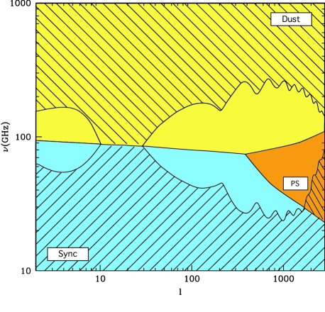
Figure 1: The dominant foreground in polarization as function of the frequency and the angular scale (synchrotron: light blue; dust: yellow; extragalactic radio sources: brown; gravitational lensing: green). Galactic foregrounds are modelled by Eq. (14)–(15) (see also Figure 2b). For extragalactic radio sources we use a flux limit of 1 Jy. Left plot: the not–shaded area is where the CMB E–mode is the dominant polarized signal. Right plot: as in the left plot but after reducing by a factor 10 the synchrotron and dust emission. Now, the not–shaded area indicates the region where the CMB B–mode (considering $r=0.1$) is higher than the foregrounds contribution.

2.1 Cosmic microwave background

The CMB B–mode power spectrum ($C_{B\ell}$) is characterized by a peak at $\ell_{p}\sim 90$, i.e. at the angular scale corresponding to the horizon at recombination. The amplitude of the spectrum is directly proportional to the cosmological parameter $r$ and is related to the energy scale of inflation: at the peak the amplitude is

$$\Delta B_{p} \equiv \bigg{[}{\ell_{p}(\ell_{p}+1)\over 2\pi}C_{B\ell_{p}}\bigg{]}^{1/2}T_{0}\sim$$ (4)

$$\sim 0.3\,r^{1/2}\,\mu{\rm K}\simeq 0.03\bigg{(}{E_{i}\over 10^{16}{\rm GeV}}\bigg{)}^{2}\,\mu{\rm K}\,.$$

At $\ell>\ell_{p}$ the spectrum rapidly decreases because gravitational waves oscillate and decay once inside the horizon. At very large scales very low B–mode polarization is also expected because, at the moment of recombination, the anisotropy quadrupole moment has not been significantly produced yet on scales larger than the horizon. However, the reionization of the Universe has the effect to partially polarize the CMB radiation and shift to lower redshift a fraction of the last scattering, producing a further peak at low $\ell$ in the spectrum. The amplitude and the position of such a peak depends on the optical depth of the Universe, $\tau$ [WMAP finds $\tau=0.17\pm 0.07$ (Spergel et al., 2003)].

In Figure 2b we report the expected values of $B_{\rm rms}$ for $r=0.1,\,10^{-2}$ and $10^{-3}$ (solid red lines). As shown in Eq. (4), it scales like $r^{1/2}$. If only very large scales are considered, $B_{\rm rms}$ is strongly dependent on $\tau$ and exceeds 0.1 $\mu$K for $\tau$ and $r>0.1$. On the contrary, at degree resolution, $\tau$ is less relevant but not negligible ($B_{\rm rms}$ increases by a factor 2 changing $\tau$ from 0 to 0.17). In the plot we consider $\tau=0.1$ (a conservative value compared to the WMAP best–fit one). The B–mode spectrum is less sensitive to other cosmological parameters. We fix those in agreement with the “concordance model” ($\Omega_{0}=1$, $\Omega_{\Lambda}=0.7$, $\Omega_{b}=0.05$ and $h=0.7$).

The detection of the CMB E–mode polarization is much easier than that of B–mode and it is even better with sub–degree resolution experiments (see Figure 1).At these angular scales, DASI (Kovac et al., 2002) achieved the first direct measure of E–mode polarization, while more recent observations have been provided by DASI (Leitch et al., 2004), CAPMAP (Barkats et al., 2005) and CBI (Readhead et al., 2004).At degree angular scales the value of $E_{\rm rms}$ is less than $1\mu$K with a polarization degree of only few per cent or less. Nevertheless, the CMB E–mode is still the dominant contribution in a wide range of frequencies, approximately between $60<\nu<150$ GHz.

Finally, we plot in Figure 2a the level of the B–mode polarization induced by the gravitational weak lensing of large scale structures (see magenta line). This estimate is obtained using the CMBFAST package.

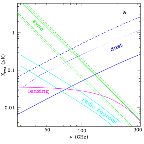
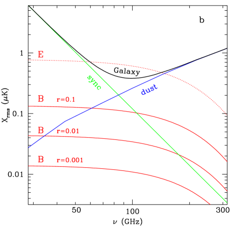
Figure 2: The rms value of foreground and CMB X=E, B modes vs. the frequency, as expected by an experiment with FWHM$\,=1\degr$.
–a– Estimates of foregrounds from different data. Synchrotron (green lines): 10$\%$–30$\%$ of the WMAP $\Delta T_{\rm rms}$ (dotted lines); estimates from Brouwn & Spoelstra data (dashed line), from high–resolution low–latitude polarization surveys (solid line) and from observations of high–latitude polarization (Abidin et al. 2003; long–dashed line). The spectral index is $\beta_{s}=-3.1$. Dust (dark blue lines): 5$\%$ of the WMAP $\Delta T_{\rm rms}$ (dashed line) and the result from the Prunet et al. (1998) model (solid line). For the frequency spectrum we consider a one–component dust model with $T=18\,K$ and emissivity $\alpha=1.7$. The dotted line is obtained by the “100$\mu$m map” (Schlegel et al., 1998) extrapolated to microwave frequencies using the model 8 of Finkbeiner et al. (1999). Radio sources (light blue lines): estimates from Tucci et al. (2004), taking the flux limit 1 and 0.2 Jy. Lensing–induced polarization (magenta line).
–b– The black solid line is the total $X_{rms}$ contribution of foregrounds, taking for the synchrotron the 20$\%$ of the WMAP estimate and $\beta_{s}=-3.1$; for the dust the model 8 of Finkbeiner et al. (1999). CMB (red lines): $E_{rms}$ (dotted line) and $B_{rms}$ (with $r=0.1,\,0.01,\,0.001$; solid lines) for the “concordance” model with $\tau=0.1$.

2.2 Synchrotron emission

Among all foregrounds, synchrotron emission is the most polarized (up to $\sim 75\%$). It is expected to be the dominant component at low frequencies ($\nu\mathrel{\mathchoice{\vbox{\offinterlineskip\halign{\hfil$\displaystyle#$\hfil\cr<\cr\sim\cr}}}{\vbox{\offinterlineskip\halign{\hfil$\textstyle#$\hfil\cr<\cr\sim\cr}}}{\vbox{\offinterlineskip\halign{\hfil$\scriptstyle#$\hfil\cr<\cr\sim\cr}}}{\vbox{\offinterlineskip\halign{\hfil$\scriptscriptstyle#$\hfil\cr<\cr\sim\cr}}}}70\,$GHz). Total–intensity data are available up to $\sim 20$ GHz, while polarization observations of the synchrotron are obtained only at few GHz or less. Estimates on the amplitude of the polarized synchrotron emission at cosmological frequencies are especially complicated for two reasons: the steepening of the spectral index that may occur at $\nu\mathrel{\mathchoice{\vbox{\offinterlineskip\halign{\hfil$\displaystyle#$\hfil\cr>\cr\sim\cr}}}{\vbox{\offinterlineskip\halign{\hfil$\textstyle#$\hfil\cr>\cr\sim\cr}}}{\vbox{\offinterlineskip\halign{\hfil$\scriptstyle#$\hfil\cr>\cr\sim\cr}}}{\vbox{\offinterlineskip\halign{\hfil$\scriptscriptstyle#$\hfil\cr>\cr\sim\cr}}}}20$ GHz, and the frequency dependence of the degree of polarization.

The synchrotron spectral index, $\beta_{s}$, is computed on nearly all sky using the surveys at 408 MHz (Haslam et al., 1982), at 1.4 GHz (Reich & Reich, 1986) and at 2.3 GHz (Jonas et al., 1998) by Giardino et al. (2002) and Platania et al. (2003). These analysis show $\beta_{s}$ to vary across the sky between $-2.5$ and $-3.0$, with an average value $<\beta_{s}>\simeq-2.7$ and a dispersion of 0.1–0.2 at sub–degree angular resolution. A relevant steepening ($<\beta_{s}>\approx-3$ out of the Galactic Plane) is found from the first–year data of WMAP at 23 GHz (Bennett et al., 2003). Bernardi et al. (2004) studied the distribution of the spectral index computed between 1.4 and 23 GHz: the frequency spectrum is observed rather flat along the Galactic Plane, whereas steeper at high Galactic latitudes with a typical value $\beta_{s}=-3.1$. A further steepening is also suggested in the 23–41 GHz range by Bennett et al. (2003), although it has to be confirmed. In the following, we shall assume $\beta_{s}=-3.1$ as the mean spectral index for the synchrotron emission at all considered frequencies.

Estimates of the rms signal of $X=E,\,B$ modes for the synchrotron emission are reported in Figure 2a (green lines). A set of estimates obtained in different ways is considered, which permits to get a range of plausible levels. First we scale down unpolarized synchotron as follow: the full–sky synchrotron map at 23 GHz, obtained from WMAP data after component separation with the Maximum Entropy Method (Bennett et al., 2003) and smoothed by a Gaussian beam with FWHM$=1{\degr}$, is used to compute the rms amplitude of temperature fluctuations at high latitudes ($|b|>20\degr$). We find $\Delta T_{\rm rms}=82.6$. From the Brouw & Spoelstra (1976) observations (the only up–to–now available data of the synchrotron polarization on a large fraction of the sky), Spoelstra (1984) found that on degree scales the fractional polarization at 1.411 GHz is typically 10–20 per cent with the highest value being 35$\%$. Taking into account that Faraday rotation can reduce the polarization degree at this frequency, we assume that synchrotron emission is polarized between a 10 and a 30 per cent as lower or upper limit. We get estimates as plotted with dotted lines in Figure 2a.

Secondly, estimates of $X_{\rm rms}$ can be directly achieved also from polarization data. Bruscoli et al. (2002) use Brouw & Spoelstra (1976) survey to compute the E– and B–mode APS in three patches with high signal–to–noise ratio centered at the latitudes $b=5{\degr},\,44.5{\degr},\,72.5{\degr}$. They find that the APS can be well approximated by a power law with a quite flat slope, $\mathrel{\mathchoice{\vbox{\offinterlineskip\halign{\hfil$\displaystyle#$\hfil\cr>\cr\sim\cr}}}{\vbox{\offinterlineskip\halign{\hfil$\textstyle#$\hfil\cr>\cr\sim\cr}}}{\vbox{\offinterlineskip\halign{\hfil$\scriptstyle#$\hfil\cr>\cr\sim\cr}}}{\vbox{\offinterlineskip\halign{\hfil$\scriptscriptstyle#$\hfil\cr>\cr\sim\cr}}}}-2$. Taking as the “average” spectrum at 1.4 GHz $C_{X\ell}=0.01\ell^{-1.8}$(K²), we find $X_{\rm rms}(1.4{\rm GHz})=0.11$K at $1\degr$ resolution (dashed line in Figure 2a). Similar results are also obtained from the analysis of high–resolution surveys at low Galactic latitudes (Duncan et al. 1997, Duncan et al. 1999, Uyaniker et al. 1999): extrapolating the polarization APS provided by Tucci et al. (2000) and Bruscoli et al. (2002) to low $\ell$s, we find $X_{\rm rms}\simeq 0.02$ K at 2.4 GHz (solid line in Figure 2a). However, these estimates probably have to be considered as upper limits because they come from observations of the Galactic Plane or of highly–polarized regions. Their very good agreement with the 30$\%$–WMAP predictions shown by Figure 2a confirms that a polarization degree up to 30$\%$ can be observed in highly–polarized area but as it may be not the typical percentage on the sky. The upper lines in Figure 2a may be somewhat pessimistic estimates.

Finally, the recent observations of the high–Galactic latitude polarization with the Effelsberg Telescope at 1.4 GHz (Abidin et al., 2003) point out structures in polarization on scales of several degrees with a fractional polarization up to 30–40$\%$ in the brightest regions and a rms $Q$ and $U$ signal of 50 mK. This value, extrapolated to WMAP frequencies, corresponds to the WMAP result with an average polarization degree of 10$\%$ (see long–dashed line). Nevertheless, as the polarization level at 1.4 GHz can be significantly reduced by Faraday depolarization, a percentage of 20$\%$ for the polarized synchrotron emission may be more realistic at microwave frequencies. The lower lines in Figure 2a are thus probably somewhat optimistic.

2.3 Dust emission

Millimetric or submillimetric measurements of the Galactic dust polarization are usually concentrated in Galactic clouds and star–forming regions with arcminutes angular resolution (e.g, Hildebrand et al. 1999, Greaves et al. 1999). They show a few per cent polarization and no clear frequency dependence. The first observations on large angular scales of the polarization of the Galactic dust emission are provided by Archeops at 353 GHz (Benoît et al., 2003). The Archeops data show a significantly large–scale polarized emission in the Galactic Plane, with a polarization degree of 4–5$\%$, with several clouds of few square degrees appearing to be polarized at more than 10$\%$.

Total–intensity observations at infrared wavelengths, where the thermal dust emission is very dominant, have been obtained by the IRAS and COBE (DIRBE) satellites. Combining these data, Schlegel et al. (1998) generated a full–sky map at 100$\mu$m with sub–degree resolution. A tentative extrapolation of the 100$\mu$m map to microwave frequencies was done by Finkbeiner et al. (1999), assuming different dust emissivity models. They use the FIRAS data in the 100–2100 GHz range to constrain dust properties. The best agreeement is met with a two–component model, consisting of a mixture of silicate and carbon–dominated grains (see Model 8 of Finkbeiner et al. 1999). Extrapolating the 100$\mu$m map to 100 GHz with this model, we find $\Delta T_{\rm rms}=7.4\,\mu$K for a $1\degr$ resolution. The dust rms intensity at this resolution can also be estimated from WMAP data: using the Galactic emission models by Bennett et al. (2003), it is found $\Delta T_{\rm rms}=13\,\mu$K at 93.5 GHz, significantly higher than the Finkbeiner et al. (1999) value. However, because in the WMAP frequency range the dust emission is only a secondary contribution, this value is still controversial. The predictions on the rms polarization presented in Figure 2a assume a typical polarization degree for the interstellar diffuse dust emission of 5$\%$, in agreement with Archeops results (dotted and dashed blue lines).

Finally, Prunet et al. (1998) provide a model of the dust polarized emission using the three–dimensional HI maps of the Leiden–Dwingeloo survey at high Galactic latitudes. Different hypothesis on dust grain properties and alignment are assumed. As main result, they estimate the dust polarization APS at 100 GHz to be $C_{X\ell}\simeq 10^{-3}\ell^{-1.4}\,(\mu$K)², corresponding to $X_{\rm rms}=0.051\,\mu$K at $1\degr$ resolution (solid line in Figure 2a). This value is significantly low compared to previous ones and require a mean polarization degree less than $1\%$ for being consistent with total–intensity results.

2.4 Extragalactic sources

Extragalactic radio sources contribute significantly to temperature and polarization fluctuations only at small angular scales. At degree scales their polarized signal is a small fraction of the total foregrounds, even if it can exceed the cosmological B–mode for a low value of $r$. Predictions on the polarization properties of radio sources at microwave frequencies and on their contamination for CMB measurements are provided by Tucci et al. (2004), using the evolutionary model of Toffolatti et al. (1998) which predicts the number counts of sources at cm and mm wavelengths. In Figure 2a we report the rms polarization assuming that all sources with flux density higher than 1 or 0.2 Jy have been completely removed (light blue lines).

At frequencies higher than 100 GHz, the contribution of dusty galaxies should also be taken into account. However, the sparsity of data on polarization at sub-mm wavelengths makes reliable predictions difficult. In any case, we expect that the polarization degree from the dust emission in external galaxies is not higher than the polarization degree observed in the Milky Way, i.e. only a few per cent. Supposing a polarization of 2$\%$ (Hildebrand, 1996; Greaves et al., 2000; Matthews & Wilson, 2002), Figure 1 shows that the dusty galaxies contribution never overcomes the other foregrounds at all frequencies lower than 1000 GHz and at $\ell<3000$. Polarization from dusty galaxies will be neglected in this work.

2.5 Other sources of polarization

Here we give a brief description of some secondary sources of polarized emission, although they will not be taken into account in the analysis.

The existence of an anomalous dust–correlated emission, far brighter than the expected thermal dust emission, has been well detected at $\sim 10$–30 GHz (e.g., Kogut et al. 1996, de Oliveira-Costa et al. 1999, Finkbeiner 2003). One possible explanation is the electric dipole emission from rapidly rotanting small dust grains, known as “spinning dust” (Draine & Lazarian, 1998). This emission is expected to be polarized if grains are aligned with the magnetic field. In any case, as shown by Lazarian & Finkbeiner (2003), the polarization is marginal for $\nu>35$ GHz. Another possibility is the magneto–dipole emission from strongly magnetized grains (Draine & Lazarian, 1999). The polarization due to this mechanism depends on the dust composition and structure, and can be substantial at microwave frequencies (Lazarian & Finkbeiner, 2003).

Finally, in the presence of a temperature quadrupole, the scattering of the CMB photons by free electrons in galaxy clusters leads to a secondary linear polarization. In addition to the primary CMB quadrupole, another important origin of temperature quadrupole is due to the peculiar velocity of clusters. However, the contribution to the B–mode polarization from this secondary signal is considerably low, several orders of magnitude below the lensing–induced polarization on the large scales (for a review, see Cooray et al. 2004).

3 Galactic foregrounds subtraction and residual power spectrum

Figure 2 clearly shows that the contribution of Galactic foregrounds to the B–mode polarization dominates over the CMB signal at all frequencies, even in the most optimistic cases. The knowledge of foreground emissions and the ability to remove them assume therefore a primary role for the possibility of observing the polarization induced by gravitational waves. Multifrequency observations are thus absolutely necessary, expecially on large scales. During last years, many methods have been suggested to perform the component separation of the microwave sky. Some of them adopt Bayesian approaches (e.g., MEM by Hobson et al. 1998 and Wiener filtering by Tegmark & Efstathiou 1996 and Bouchet & Gispert 1999 ) whereas others blind techniques (e.g., SMICA by Delabrouille et al. 2003a and FastICA by Maino et al. 2002). In this work we do not want to go into details of different techniques and assumptions for the components separation. Our aim is to estimate the level of residual Galactic foregrounds left in the clean maps after their subtraction. We make the following hypotheses: i) a template for synchrotron and dust emission (the only Galactic foregrounds considered) is available; ii) their spectral behaviour is estimated in the frequency range of interest. A linear subtraction of Galactic foregrounds is then employed extrapolating templates to the “cosmological” frequency. The instrumental noise present in templates and the uncertainty on the frequency spectrum of foregrounds are taken into account in order to compute the residual polarization. Compared to standard techniques for component separation, this method is, in principle, less accurate. However, it provides qualitative estimates for the residual foregrounds that are good enough for the aim of this work. Moreover, its simplicity allows to compute analytically the power spectrum of residual Galactic contaminants and, in addition, the method only requires minimal assumptions on the foregrounds and their statistical properties.

Let $\nu_{o}$ be the frequency chosen to detect the CMB polarization (hereafter called the “observational frequency”) and $\nu_{t}$ the frequency of the template for the Galactic foreground we want to subtract. We suppose that the foreground frequency spectrum can be approximated by a power law (at least between $\nu_{t}$ and $\nu_{o}$):

$$I_{\nu_{o}}=I_{\nu_{t}}\Big{(}{\nu_{o}\over\nu_{t}}\Big{)}^{-\beta}\,.$$ (5)

In general, the value of the spectral index $\beta$ is expected to change with the sky position. We indicate with $\tilde{I}_{\nu_{t}}({\bf\hat{n}})$ and $\tilde{\beta}({\bf\hat{n}})$ the template foreground intensity and the measured spectral index in the sky direction ${\bf\hat{n}}$, while the difference between these quantities and the actual ones is $\Delta I_{\nu_{t}}({\bf\hat{n}})$ and $\Delta\beta({\bf\hat{n}})$ respectively. If we extrapolate the template to the observational frequency using Eq. (5), the residual foreground left in the map at $\nu_{o}$ after foreground subtraction is:

$$\Delta I_{\nu_{o}}({\bf\hat{n}})=I_{\nu_{o}}({\bf\hat{n}})-\tilde{I}_{\nu_{o}}({\bf\hat{n}})=$$

$$(\tilde{I}_{\nu_{t}}+\Delta I_{\nu_{t}})({\bf\hat{n}})\Big{(}{\nu_{o}\over\nu_{t}}\Big{)}^{-[\tilde{\beta}({\bf\hat{n}})+\Delta\beta({\bf\hat{n}})]}-\tilde{I}_{\nu_{t}}({\bf\hat{n}})\Big{(}{\nu_{o}\over\nu_{t}}\Big{)}^{-\tilde{\beta}({\bf\hat{n}})}=$$

$$\tilde{I}_{\nu_{o}}({\bf\hat{n}})\Big{[}\Big{(}{\nu_{o}\over\nu_{t}}\Big{)}^{-\Delta\beta({\bf\hat{n}})}-1\Big{]}+\Delta I_{\nu_{t}}({\bf\hat{n}})\Big{(}{\nu_{o}\over\nu_{t}}\Big{)}^{-[\tilde{\beta}({\bf\hat{n}})+\Delta\beta({\bf\hat{n}})]}\,.$$ (6)

Keeping only first order terms, Eq. (6) is reduced to

$$\Delta I_{\nu_{o}}({\bf\hat{n}})\simeq\ln\Big{(}{\nu_{t}\over\nu_{o}}\Big{)}\tilde{I}_{\nu_{o}}({\bf\hat{n}})\Delta\beta({\bf\hat{n}})+\Delta I_{\nu_{t}}({\bf\hat{n}})\Big{(}{\nu_{o}\over\nu_{t}}\Big{)}^{-\tilde{\beta}({\bf\hat{n}})}\,.$$ (7)

As expected, the residual foreground in direction ${\bf\hat{n}}$ consists in a part proportional to the uncertainty on the spectral index, and another proportional to the error (or noise) on the foreground polarization at the template frequency. Extending this result to the case of polarization measurements is trivial:

$$\Delta(Q\pm iU)_{\nu_{o}}({\bf\hat{n}}) \simeq \ln\Big{(}{\nu_{t}\over\nu_{o}}\Big{)}(\tilde{Q}\pm i\tilde{U})_{\nu_{o}}({\bf\hat{n}})\Delta\beta({\bf\hat{n}})+$$ (8)

$$\Delta(Q\pm iU)_{\nu_{t}}({\bf\hat{n}})\Big{(}{\nu_{o}\over\nu_{t}}\Big{)}^{-\tilde{\beta}({\bf\hat{n}})}\,.$$

Assuming that no correlation exists between the errors on $\beta$ and $Q\pm iU$ and their estimated values, the $X=E,\,B$ modes APS of the residual polarization is the sum of the two terms in Eq. (8). The former (indicated by $C^{\mathcal{R}_{1}}_{X\ell}$) is obtained by the convolution of the spectrum of the estimated foreground polarization at $\nu_{o}$, $C_{X\ell}^{f}$, with that of the uncertainty on the spectral index $\Delta\beta$, $C^{\beta}_{\ell}$. The mathematical calculations are reported in Appendix A. We get

$$C^{\mathcal{R}_{1}}_{X\ell}={A^{2}\over 16\pi}\sum_{\ell_{1}}(2\ell_{1}+1)C^{f}_{X\ell_{1}}\mathcal{F}(\ell,\ell_{1})\,,$$ (9)

where $A\equiv\ln(\nu_{t}/\nu_{o})$ and

$$\mathcal{F}(\ell,\ell_{1})=\sum_{\ell_{2}}(2\ell_{2}+1)C^{\beta}_{\ell_{2}}\Big{(}{\ell\atop 2}{\ell_{1}\atop-2}{\ell_{2}\atop 0}\Big{)}\Big{(}{\ell\atop 2}{\ell_{1}\atop-2}{\ell_{2}\atop 0}\Big{)}$$

(the last two terms are the Wigner 3j–Symbols). In principle, a convolution is required also for the second term of Eq. (8), $C^{\mathcal{R}_{2}}_{X\ell}$. However, keeping again only first order terms (in particular, we replace $\tilde{\beta}({\bf\hat{n}})$ with the average value of the spectral index, $\langle\tilde{\beta}\rangle$) and supposing the polarization uncertainty in the template to behave like a white noise, we find that

$$C^{\mathcal{R}_{2}}_{E,B\ell}=C_{\ell}^{N}\Big{(}{\nu_{o}\over\nu_{t}}\Big{)}^{-2\langle\tilde{\beta}\rangle}\,,$$ (10)

where $C_{\ell}^{N}=\Omega_{pix}\sigma^{2}_{t}$ is the white–noise spectrum in the template map ($\Omega_{pix}$ is the solid angle per pixel and $\sigma_{t}$ the noise per pixel in polarization).

The hypothesis of a power–law frequency spectrum is not quite true for the dust emission. It can be better modelled by a law as $I_{\nu}\propto\nu^{\beta}B_{\nu}(T)$, where $B_{\nu}(T)$ is the Planck function at temperature $T$ of dust grains. Then, for the dust emission we replace Eq. (5) by

$$I_{\nu_{o}}=I_{\nu_{t}}\Big{(}{\nu_{o}\over\nu_{t}}\Big{)}^{-\beta}{e^{h\nu_{t}/KT}-1\over e^{h\nu_{o}/KT}-1}\,.$$ (11)

We can assume the temperature of grains to be constant over all the sky and the spatial changes in the frequency spectrum to be restricted only to the value of $\beta$. The residual power spectra for the dust emission will be still given by Eq. (9), but multiplied by the factor $[(e^{h\nu_{t}/KT}-1)/(e^{h\nu_{o}/KT}-1)]^{2}$, that is $\sim 2$ for $T=18$ K, $\nu_{o}=100$ GHz and $\nu_{t}=140$ GHz.

Figure 3: Residual polarization spectra $C^{\mathcal{R}_{1}}_{X\ell}$ under the hypothesis of average (C1; solid line) and pixel–dependent (C2; dashed line) spectral index for Galactic foregrounds. The dotted line is a power law normalized to the unity and with slope $-1.8$.

3.1 Residual power spectrum due to spectral index uncertainties

In order to estimate the power spectrum of the residual foreground polarization by Eq. (9)–(10), the knowledge of three angular spectra is required: $C^{f}_{X\ell}$ (polarization spectrum of the Galactic foregrounds which can be directly computed from the template maps); $C^{N}_{\ell}$ (spectrum of the white noise in foreground templates); $C^{\beta}_{\ell}$ (spectrum of the spectral index error). Here, we focus on the latter which is the most critical to define the behaviour of $C^{\mathcal{R}_{1}}_{X\ell}$. We consider two different extreme cases:

(C1) Average spectral index: the template for a Galactic foreground can be extrapolated to the observational frequency using the sky–average spectral index. In this case, the error on the spectral index will be the difference between $\beta({\bf\hat{n}})$ and the estimated average value $\langle\tilde{\beta}\rangle=\langle\beta\rangle$ (assuming no systematic effect in the estimation). Because the spectral index of Galactic emissions is directly related to physical conditions of the region where the emission is produced both for synchrotron (spectral index depends on the energy distribution of electrons) and for dust emission (dependent on the temperature and the emissivity of grains), we expect that maps of $\beta({\bf\hat{n}})$ and, consequently, of the error $\Delta\beta({\bf\hat{n}})$ show coherent structures like those observed in total–intensity templates. This is visually observed comparing the maps of the synchrotron spectral index provided by Giardino et al. (2002) and Bernardi et al. (2004) and the total–intensity ones. More quantitatively, we estimate the power spectrum of $\beta({\bf\hat{n}})$ obtained by Giardino et al. (2002) from low–frequency surveys, and we find a power law spectrum with a slope of $\sim-3$, in agreement with the behaviour of the synchrotron intensity spectra (Tegmark & Efstathiou 1996; Bouchet et al. 1996; Bouchet & Gispert 1999). We expect it is same for the dust emission.

Therefore, in this case (C1) we assume that $C^{\beta}_{\ell}$ is proportional to the total–intensity APS for the Galactic foregrounds. The normalization of $C^{\beta}_{\ell}$ is obtained by fixing the dispersion of the spectral index around its average value, $\sigma_{\beta}$, and using the relation: $\sigma^{2}_{\beta}=\sum_{\ell}(2\ell+1)C^{\beta}_{\ell}W_{\ell}/4\pi$, where $W_{\ell}$ is the window function corresponding to the resolution at which the dispersion $\sigma_{\beta}$ has been computed.

The residual power spectrum $C^{\mathcal{R}_{1}}_{X\ell}$ obtained under this hypothesis is shown as solid line in Figure 3. Hereafter, we take: $C^{\beta}_{\ell}\propto\ell^{-3}$ and $\sigma_{\beta}=0.2$, in agreement with the results found by Giardino et al. (2002) and Bernardi et al. (2004) for the synchrotron emission at high Galactic latitudes, and by WMAP measurements for the dust spectral index (see Figure 9 of Bennett et al. 2003). The polarization spectra of the Galactic foregrounds are assumed to be of the form $C^{f}_{X\ell}=\ell^{-1.8}$. Both spectra are smoothed by a window function with FWHM$=1\degr$. We notice that the residual spectra $C^{\mathcal{R}_{1}}_{X\ell}$ have the same slope of the foreground polarization spectra as expected (except for the first $\ell$s), but with an amplitude a factor $\sim$100 lower [here we have considered $A=1$ in Eq. (9)].

(C2) Pixel dependent spectral index: as second case, we consider that the foreground template is extrapolated to the observational frequency using a spectral index estimated pixel by pixel. Moreover, we suppose that the error on these spectral indeces, $\Delta\beta({\bf\hat{n}})$, behaves like a white noise. Consequently its power spectrum $C^{\beta}_{\ell}$ will be constant. The amplitude of $C^{\beta}_{\ell}$ clearly depends on the noise in data used to compute the spectral index. As working case, we assume that the average error on spectral index is equal to the dispersion in the spectral index distribution, i.e. the above value $\sigma_{\beta}=0.2$. Even if this assumption is probably very conservative, it is however interesting because it allows us a direct comparison to results of case C1, as the total power of the error is the same, but distributed differently in $\ell$. Figure 3 (dashed line) shows that the residual APS behaves like a white noise spectrum (at least up to the resolution scale) with a very small amplitude at large angular scales: at $\ell<10$ it is $10^{-5}$–$10^{-6}$ times lower than $C^{f}_{X\ell}$, and two orders of magnitude lower than predictions for case C1. Considering that the power of the CMB B–mode polarization is concentrated at degree scales ($\ell<100$), this second case for foreground subtraction is much more favourable, removing particularly well the Galactic foregrounds on the largest angular scales.

Figure 4: Polarization power spectra at 100 GHz (in thermodynamic temperature): CMB E–mode (upper solid line) and B–mode for $r=0.1$ and $10^{-4}$ (lower solid lines); synchrotron (left plot, dashed lines); dust (right plot, dashed lines); gravitational lensing (dotted lines); extragalactic radio sources with $S<1$ Jy (short dashed lines). The thick dashed lines show the residual contribution of the synchrotron and dust emission after their subtraction, following the two schemes described in sec. 3. In these spectra the effect of the beam (FWHM$=1\degr$) start to be noticed at $\ell\sim 100$.

4 Uncertainty on the tensor–to–scalar perturbations ratio in an ideal experiment including foregrounds

The main goal of CMB observations is to estimate the angular power spectrum. Its amplitude and shape allows us to have information on cosmological parameters. The precision achieved for a parameter can be estimated from the Fisher matrix. The CMB polarization is usually described by E and B–mode and their relative spectra; for polarization measurements the cosmological parameter estimation using the Fisher matrix is given by

$$\mathcal{F}_{ij}=\sum_{\ell}\bigg{(}{1\over\Delta C_{E\ell}^{2}}{\partial C_{E\ell}\over\partial\alpha_{i}}{\partial C_{E\ell}\over\partial\alpha_{j}}+{1\over\Delta C_{B\ell}^{2}}{\partial C_{B\ell}\over\partial\alpha_{i}}{\partial C_{B\ell}\over\partial\alpha_{j}}\bigg{)}$$ (12)

where $\alpha_{i}$ are the cosmological parameters to be estimated. The diagonal terms of the inverse of the Fisher matrix provide the minimum possible variance for the parameter $\alpha_{i}$, i.e. $(\delta\alpha_{i})^{2}=\mathcal{F}^{-1}_{ii}$. The quantity $\Delta C_{X\ell}$ is the uncertainty on the $X=E,\,B$ power spectra at the multipole $\ell$:

$$\Delta C_{X\ell}^{2}={2\over(2\ell+1)f_{sky}}(C_{X\ell}+N_{X\ell})^{2}\,,$$ (13)

where $f_{sky}$ is the fraction of the sky observed by the experiment. Beside the cosmic variance, the uncertainty on $C_{X\ell}$ arises from the noise term $N_{X\ell}$, which includes the instrumental noise and the foregrounds contamination, treated as an extra source of noise.

As we have previously discussed, the CMB polarization at degree scales depends strongly on two cosmological parameters, the tensor–to–scalar ratio $r$ and the optical depth of the Universe $\tau$. Polarization spectra are affected also by other parameters, but polarization measurements are of particular importance only for $r$ and $\tau$, which can be at best poorly constrained with temperature. Therefore, we consider in the Fisher matrix only parameters $\alpha_{i}=\{\tau,\,r\}$, all the other cosmological parameters being supposed to be already known. The results on the tensor–to–scalar ratio are given in terms of the quantity $r_{lim}$, defined as the value of $r$ under which the relative error on $r$ is 0.3 (i.e., corresponding to about a 3–$\sigma$ error). On the contrary, the uncertainty on the parameter $\tau$ will be not discussed, being its value generally estimated with a high precision, less than $10\%$, in almost all the cases we have considered.

We consider as reference experiment a full–sky experiment with a resolution of FWHM=$1\degr$ and a negligible level of instrumental noise (“noise–free”). A Galactic Plane cut is applied and $f_{sky}=0.8$ is used in the analysis. The observational frequency, aimed to detect the gravitational wave polarization, is choosen at $\nu=$100 GHz, which corresponds to the frequency where the Galactic polarized emission is expected to be minimum (see Figure 2). We model the polarization of Galactic foregrounds using a power–law angular spectrum: at 100 GHz, in antenna temperature, the synchrotron spectrum is

$$C_{X\ell}=1.2\times 10^{-2}\ell^{-1.8}\,(\mu K^{2})\,,$$ (14)

giving $X_{\rm rms}=0.12\,\mu$K at $1\degr$ resolution (the normalization is based on the WMAP results and a polarization degree of 20$\%$ ); for the dust polarization

$$C_{X\ell}=1.6\times 10^{-2}\ell^{-1.4}\,(\mu K^{2})\,,$$ (15)

corresponding to 0.26$\,\mu$K at $1\degr$ resolution (as expected by the Finkbeiner et al. (1999) model with a polarization degree of 5$\%$). These spectra, compared to the CMB E and B–mode ones, are plotted in Figure 4.

We suppose that Galactic foregrounds are subtracted from data at 100 GHz using the prescriptions described in the previous section. In particular, we consider that a template for the synchrotron polarized emission is available at $\nu=60$ GHz and one for the dust at 140 GHz. Under these conditions and supposing noise–free templates, the noise term in Eq. (13) is given only by the residual Galactic polarization, $C^{\mathcal{R}_{1}}_{X\ell}$ (thick dashed lines in Figure 4), and extragalactic foregrounds. The rms amplitude of the Galactic polarization is reduced by a factor 20 or 60, according to the subtraction scheme used.

4.1 Constraints on $r$ imposed by Galactic foregrounds

The Fisher matrix is used to estimate the uncertainty on $r$ for our reference experiment. No contribution from extragalactic sources is taken into account. The results are shown in Figure 5. The two different methods to subtract Galactic foregrounds are considered: in C1 case (the frequency spectrum for Galactic emissions is considered independently of the sky position) we find $r_{lim}=8.3\times 10^{-5}$; a detection of the tensor polarization with lower amplitude can be achieved if the spectral law is estimated pixel by pixel (C2 case). In particular, a 3–$\sigma$ detection is possible for $r=1.8\times 10^{-5}$. These very low values for $r_{lim}$ tell us that the Galactic foregrounds are subtracted in a very efficient way in both cases (as expected when the noise is negligible).

No improvement of the sensitivity on $r$ is observed increasing the instrumental resolution to angular scales smaller than $1\degr$, confirming that all the information on the cosmological $B$–mode comes from $\ell\mathrel{\mathchoice{\vbox{\offinterlineskip\halign{\hfil$\displaystyle#$\hfil\cr<\cr\sim\cr}}}{\vbox{\offinterlineskip\halign{\hfil$\textstyle#$\hfil\cr<\cr\sim\cr}}}{\vbox{\offinterlineskip\halign{\hfil$\scriptstyle#$\hfil\cr<\cr\sim\cr}}}{\vbox{\offinterlineskip\halign{\hfil$\scriptscriptstyle#$\hfil\cr<\cr\sim\cr}}}}100$. If the resolution is reduced to FWHM$=7\degr$, we find that $r_{lim}$ gets clearly worse only in the C1 case. On the contrary, the C2 results appear to be nearly independent of the resolution at least for FWHM$\leq 7\degr$, meaning that the largest scales ($\ell\mathrel{\mathchoice{\vbox{\offinterlineskip\halign{\hfil$\displaystyle#$\hfil\cr<\cr\sim\cr}}}{\vbox{\offinterlineskip\halign{\hfil$\textstyle#$\hfil\cr<\cr\sim\cr}}}{\vbox{\offinterlineskip\halign{\hfil$\scriptstyle#$\hfil\cr<\cr\sim\cr}}}{\vbox{\offinterlineskip\halign{\hfil$\scriptscriptstyle#$\hfil\cr<\cr\sim\cr}}}}30$) are enough to provide a good detection of $r$. For a low–resolution experiment, the loss of information from $\ell\sim 100$ is probably balanced by a decrease of the amplitude of $C^{\mathcal{R}_{1}}_{X\ell}$.

Finally, we have verified that previous results are nearly insensitive to the value of the optical depth. In fact, the reionization affects the B–mode APS only for $\ell\mathrel{\mathchoice{\vbox{\offinterlineskip\halign{\hfil$\displaystyle#$\hfil\cr<\cr\sim\cr}}}{\vbox{\offinterlineskip\halign{\hfil$\textstyle#$\hfil\cr<\cr\sim\cr}}}{\vbox{\offinterlineskip\halign{\hfil$\scriptstyle#$\hfil\cr<\cr\sim\cr}}}{\vbox{\offinterlineskip\halign{\hfil$\scriptscriptstyle#$\hfil\cr<\cr\sim\cr}}}}10$, where the cosmic variance strongly constrains the precision on the $r$ detection. Hereafter, the results are given for $\tau=0.1$.

Figure 5: Fractional errors of $r$ as function of $r$ for the reference experiment (full–sky, “noise–free” and FWHM$=1\degr$) in the two hypothesis on $C^{\beta}_{\ell}$: C1 (solid line) and C2 (dot–dashed line). Dashed line (C1 case) and dotted line (C2 case) are for the same experiment but with FWHM$=7\degr$. Only Galactic foregrounds are considered.

4.2 Effects of the extragalactic B–mode polarization on $r_{lim}$

The next question is how much extragalactic radio sources and the polarization induced by gravitational weak lensing can affect the estimate of $r_{lim}$. At degree scales they provide only a secondary contribution to the B–mode polarization compared to the Galactic emissions. At 100 GHz, the radio–sources and lensing–induced B–mode spectra are constant with nearly the same amplitude, at least up to $\ell\mathrel{\mathchoice{\vbox{\offinterlineskip\halign{\hfil$\displaystyle#$\hfil\cr<\cr\sim\cr}}}{\vbox{\offinterlineskip\halign{\hfil$\textstyle#$\hfil\cr<\cr\sim\cr}}}{\vbox{\offinterlineskip\halign{\hfil$\scriptstyle#$\hfil\cr<\cr\sim\cr}}}{\vbox{\offinterlineskip\halign{\hfil$\scriptscriptstyle#$\hfil\cr<\cr\sim\cr}}}}300$. However, as shown in Figure 4, multifrequency experiments allow us to remove efficiently the Galactic foregrounds from polarization maps, and thus extragalactic polarization becomes the greatest contribution to the B–mode also at very large scales. Observations at different frequencies are not useful for the subtraction of point sources or of the lensing–induced polarization, that require experiments with arcminute resolution. They become a critical problem for low–resolution experiments.

4.2.1 Extragalactic radio sources

In the last years, a large effort has been done to develop methods able to detect extragalactic point sources in CMB maps and to estimate their intensity emission (e.g., Tegmark & Oliveira-Costa 1998, Sanz et al. 2001, Vielva et al. 2003). Complete catalogues of extragalactic sources with low flux limits are expected to be extracted from the forthcoming data. For example, Vielva et al. (2003), using a method based on the Spherical Mexican Hat Wavelet, showed that 90$\%$–completed catalogues up to $\sim 200$ mJy can be extracted by Planck observations at the frequencies of 100, 143 and 217 GHz. At the moment, these techniques have not been extended yet to polarization maps.

In any case, because we are only interested to reduce the contribution of point sources to the polarization maps, the best strategy is to exploit the total–intensity catalogues in order to mask all the pixels with bright sources. Supposing that total–intensity catalogues of radio sources will be available up to very low flux limits, the only restriction is given by the number of pixels that can be masked in a map without losing too much information. This is a strong constraint expecially for low–resolution experiments. We fix in the ten per cent the maximum percentage of beam–size pixels we can mask. For a full–sky experiment with FWHM$=1\degr$ (like the reference experiment), it corresponds to 3300 pixels, taking into account the Galactic Plane cut. According to the number counts of Toffolatti et al. (1998) model, the same number of radio sources is found at 100 GHz for fluxes $S\geq 150$ mJy.

Thus, we compute the relative error on $r$ in the hypothesis that all the sources with $S>150$ mJy have been masked (the APS amplitude of the remaining radio sources is $7.2\times 10^{-8}\,\mu$K²). We find $r_{lim}=1.4\times 10^{-4}$ and $6\times 10^{-5}$ in the cases C1 and C2 respectively (see Figure 6). In this figure we report also the results obtained if only the sources with $S\geq 1$ Jy are removed. We stress that as the contribution of extragalactic sources becomes higher the $r_{lim}$ value is less affected by the amplitude of the residual Galactic polarization.

Because the contribution of radio sources tends to decrease at frequencies higher than 100 GHz, it is interesting to study what occurs when the observational frequency is increased, $\nu_{o}>100$ GHz. We have considered $\nu_{o}=140$ GHz and the Galactic foreground templates at 60 and 220 GHz. However, the resulting $r_{lim}$ get significantly worse than in the reference case, confirming that $100$ GHz is an appropriate frequency to detect the CMB B–mode polarization with this foreground subtraction scheme.

Figure 6: Fractional error of $r$ for the reference experiment, considering the two different schemes of Galactic foregrounds subtraction (C1, left plot; C2, right plot). The contribution of radio sources with $S<150$ mJy (solid lines) and $S<1$Jy is included (dashed lines). Previous results with no contribution from extragalactic foregrounds are shown as the dotted line.

Figure 7: Fractional error of $r$ for the reference experiment, considering the two different schemes of Galactic foregrounds subtraction (C1, left plot; C2, right plot). We include the contribution of the lensing–induced polarization: the total one (dashed lines) and reduced by a factor 10 (solid lines). No contribution from extragalactic foregrounds is considered as the dotted line.

4.2.2 Gravitational lensing

The decontamination of B–mode polarization maps from the polarization induced by gravitational weak lensing can be achieved reconstructing the projected mass distribution of large scale structures (or the lensing potential). Hu & Okamoto (2002) showed that the best estimator for the projected mass distribution is provided by the correlation between the CMB E and B–modes, which allows us to reconstruct the distribution power spectrum up to multipoles of $\ell\sim 1000$. Different approaches have been suggested by Knox & Song (2002), Kesden et al. (2002) and Seljak & Hirata (2003): they show that a high precision in the lensing reconstruction can be obtained only for low–noise experiments with arcminute resolution. In particular, Table 1 of Seljak & Hirata (2003) provides the residual B–mode contamination as a function of the beam size and of the instrumental noise. The lensing “noise” always decreases when instrumental noise and/or the resolution are improved. The authors suggest that in an ideal condition of a free–noise experiment with unlimited resolution the lensing contamination could be removed completely. On the contrary, they argue that for wide beam detectors (FWHM$>20^{\prime}$) the cleaning methods are practically useless.

So far, we have considered that the typical polarization experiment is full–sky with degree resolution. In this case, the lensing contamination can become the dominant limitation for detecting the gravitational waves polarization with low values of $r$. A 3–$\sigma$ detection, in fact, is possible only for $r\mathrel{\mathchoice{\vbox{\offinterlineskip\halign{\hfil$\displaystyle#$\hfil\cr>\cr\sim\cr}}}{\vbox{\offinterlineskip\halign{\hfil$\textstyle#$\hfil\cr>\cr\sim\cr}}}{\vbox{\offinterlineskip\halign{\hfil$\scriptstyle#$\hfil\cr>\cr\sim\cr}}}{\vbox{\offinterlineskip\halign{\hfil$\scriptscriptstyle#$\hfil\cr>\cr\sim\cr}}}}4\times 10^{-4}$ if the lensing noise is not subtracted (see dashed lines in Figure 7). On the other hand, information from high–resolution experiments can be exploited: the Planck mission and upcoming ground–based experiments are expected to be able to measure the lensing–induced B–mode APS with a good precision (Bowden et al. 2004, Ganga 2004). In the hypothesis that the lensing–induced spectrum can be reduced by a factor of 10 [as indicated by Knox & Song (2002) for his reference experiment], the previous results are improved significantly, expecially in the C2 hypothesis, for which we get $r_{lim}\simeq 5\times 10^{-5}$ (see Figure 7).

Figure 8: Fractional errors of $r$ for the reference experiment, including all foregrounds: the two schemes for the Galactic polarization subtraction are considered (C1, solid line; C2, dot–dashed line). Dashed line (C1) and dotted line (C2) are for a small–area experiment without extragalactic contributions.

4.3 Limits on $r$ including all foregrounds

Finally, we show in Figure 8 the results on $\Delta r/r$ taking into account the following foreground contributions: 1) the residual Galactic polarized emission; 2) the contribution from extragalactic radio sources with flux $S<150$ mJy; 3) the polarization induced by weak lensing, but with its power spectrum reduced by a factor 10. For the reference experiment we obtain $r_{lim}\simeq 9\times 10^{-5}$ ($1.8\times 10^{-4}$), using the C2 (C1) spectrum for the residual Galactic polarization. We want to stress again that, when extragalactic foregrounds are included, the value of $r_{lim}$ is nearly independent of the method (and hypothesis) employed for removing the Galactic foregrounds polarization. If we were able to completely subtract the Galactic emission, the resulting $r_{lim}$ (under previous conditions) would be $7\times 10^{-5}$, not far from the above values. It means that the limit of $r\sim 10^{-4}$ on the detectability of the polarization produced by gravitational waves is due essentially to radio sources and lensing, even in the case of a raw Galactic foregrounds subtraction (as in the C1 scheme).

When extragalactic contributions are included, low–resolution experiments are much less effective to estimate $r$. In particular, extragalactic radio sources are a serious problem due to the difficulty to detect and subtract them. For example, considering FWHM=$7\degr$, we find $r_{lim}\sim 10^{-3}$ in the best case.

4.3.1 High–resolution, small–area experiment

An experiment with arcminute resolution could overcome the constraints imposed by extragalactic foregrounds. In fact, on the one hand, the number of arcminute pixels that can be masked to remove radio sources is much higher, reducing the flux limit to $\ll 150$ mJy and making their contribution negligible (also in a small area); on the other hand, the high resolution (with the “noise–free” condition) allows us to reconstruct with high precision the lensing B–mode power spectrum directly from the data (Seljak & Hirata, 2003). In particular, we study what occurs for an experiment covering a sky area of $30\degr\times 30\degr$ in the hypothesis of a perfect subtraction of extragalactic foregrounds: the limited sky area strongly constrains the detectability of the tensor polarization, due to the cosmic variance on the low $\ell$ (we remind that the uncertainty on $r$ increases proportionally to $f_{sky}^{-1/2}$). Only if Galactic foregrounds are removed in an accurate way, as under the C2 conditions, $r_{lim}$ is similar to that found for a full–sky experiment (see the dotted line in Figure 8).

5 Results from future experiments

In this section we apply the previous analysis to experiments characterized by a given sensitivity to the polarized emission. Practically, it means to include the instrumental sensitivity in the noise term of the Fisher matrix. We also take into account the noise in template maps in order to estimate the APS of the residual Galactic polarization, by adding the term given in Eq. (10).

In the next years, a large number of experiments has been planned with the explicit objective to measure the CMB polarization (for a review on the polarization experiments see Delabrouille et al. 2003b). However, while they may provide an accurate estimate of the E–mode power spectrum both at large and small angular scales, for the forthcoming experiments the detection of the gravitational waves polarization is still a challenge and it will be possible only for high values of the tensor–to–scalar ratio $r$.

In the mid term, the Planck mission satisfies the best conditions to search the “inflationary” polarization: a full–sky coverage and a good characterization of all the relevant foregrounds. In fact, a large frequency range is spanned and more than one frequency is dedicated to the study of the Galactic foregrounds, providing adequate knowledge of their spectral behaviour and template maps in polarization. On the other hand, the arcminutes resolution allows to detect point sources up to quite low fluxes and to have a first estimate of the gravitational lensing contribution. Nevertheless, the instrumental noise is still a very strong constraint: the sensitivity to Stokes parameters $Q$ and $U$ per square degree pixel is higher than 1 $\mu$K at all the frequencies (after 14 months), significantly higher than the expected rms value for the cosmological B–mode polarization. Taking the 100 GHz channel as the “observational frequency” (and using the 30 and 217 GHz channels as templates for the synchrotron and dust emission respectivelly), we find that a 2–$\sigma$ detection of the gravitational waves polarization is possible for $r\simeq 0.05$. This result does not change if we do not include the contribution of foregrounds.

Figure 9: The value of $r_{lim}$ for an experiment like Planck, but with a sensitivity improved by a factor $\sigma/\sigma_{Planck}$. In the upper (lower) line Galactic foregrounds are subtracted following the C1 (C2) scheme and extragalactic foregrounds are partially (completely) removed.

The research of the gravitational waves polarization is also promising using ground–based experiments. As discussed above, the disadvantage of covering a limited area of the sky can be partially compensated by the high resolution, which permits a better control of the contribution provided by extragalactic sources and gravitational lensing. Experiments like PolarBear (see Ganga 2004), Clover (Taylor et al., 2004) or QUIET (Miller, 2004) are planned to achieve a very good sensitivity, of the order of $0.1\,\mu$K or less, using arrays of 1000s of detectors in only two or three frequency channels. As example, we discuss in detail the case of PolarBear: it will operate at the frequencies 90, 150 and 220 GHz covering 225 square degrees; the number of detectors for each frequency should be 400, 600 and 200 with a sensitivity per detector of 310, 345 and 640 $\mu$Ks^1/2 respectively. Considering an observational time of 1.5 years with an efficiency of 30$\%$, the sensitivity per $1\degr$ pixel at 90 GHz would be $\simeq 0.1\,\mu$K, an order of magnitude lower than the Planck one. We find that PolarBear will be able to provide a 2–$\sigma$ detection of the tensor polarization for $r\simeq 0.07$.

Based on the above experiments, we describe below the possible features for future missions specifically dedicated to the detection of the CMB B–mode polarization, and we compute the corresponding detectability limit on $r$.

Space experiment: it is interesting to know how the detectability limit on $r$ improves when reducing the instrumental noise in the Planck experiment by the same factor at all the frequencies. Figure 9 shows the results for $r_{lim}$. In the upper line we are supposing that Galactic foregrounds are subtracted following the C1 scheme and extragalactic foregrounds are partially reduced (as discussed in Sec. 4.3). This is probably an upper limit. On the other hand, in the lower line extragalactic foregrounds are neglected (we consider they are completely removed), while the C2 scheme is used for the Galactic polarization subtraction. We observe that the results are independent of the two hypothesis on the foregrounds subtraction if Planck–detectors sensitivity is improved by a factor $\mathrel{\mathchoice{\vbox{\offinterlineskip\halign{\hfil$\displaystyle#$\hfil\cr<\cr\sim\cr}}}{\vbox{\offinterlineskip\halign{\hfil$\textstyle#$\hfil\cr<\cr\sim\cr}}}{\vbox{\offinterlineskip\halign{\hfil$\scriptstyle#$\hfil\cr<\cr\sim\cr}}}{\vbox{\offinterlineskip\halign{\hfil$\scriptscriptstyle#$\hfil\cr<\cr\sim\cr}}}}30$ (corresponding to $r_{lim}\mathrel{\mathchoice{\vbox{\offinterlineskip\halign{\hfil$\displaystyle#$\hfil\cr>\cr\sim\cr}}}{\vbox{\offinterlineskip\halign{\hfil$\textstyle#$\hfil\cr>\cr\sim\cr}}}{\vbox{\offinterlineskip\halign{\hfil$\scriptstyle#$\hfil\cr>\cr\sim\cr}}}{\vbox{\offinterlineskip\halign{\hfil$\scriptscriptstyle#$\hfil\cr>\cr\sim\cr}}}}10^{-3}$). In this case, the instrumental noise is still the most constraining contribution. For sensitivities 100 times or more better than the Planck one, the upper line is constant with $r_{lim}\simeq 3.5\times 10^{-4}$, while the lower line still decreases reaching a $r_{lim}$ similar to the free–noise case for $\sigma/\sigma_{Planck}\sim 10^{-3}$. We plot the tail of the lower curve as a dotted line in order to indicate that, for so high sensitivities, it must not be considered a lower limit for the detectability of $r$, since the uncertainty of foregrounds spectral index we used, $\sigma_{\beta}=0.2$, can be improved.

We discuss now a more concrete example for a space experiment: a total of 10,000 detectors in three channels at 100, 140 and 220 GHz with the same sensitivity of Planck detectors. With about 3,000 detectors for each channel, instead of 8 present in Planck, we expect the sensitivity to increase by a factor of about 20. The 100 GHz channel is used as observational frequency and the other two channels to remove the dust polarized contribution. A template for the synchrotron polarization is also required, being its signal still important at 100 GHz. If the low–frequency channels of the Planck mission are considered, we find $r_{lim}\simeq 2.5\times 10^{-3}$. In spite of the low accuracy in the synchrotron subtraction, $r_{lim}$ is only a factor $\sim 1.4$ higher than the corresponding value of Figure 9. The results are not affected by the contribution of extragalactic foregrounds (radio sources and lensing), while only a slight dependence is noticed on the scheme of the Galactic foregrounds subtraction.

Ground Based Bolometers: an array of 5,000 bolometers at the frequencies 90 and 150 GHz with a sensitivity per detector of 250 $\mu$Ks^1/2. After one year of observations (60$\%$ efficiency) over a $30\degr\times 30\degr$ patch of the sky, we obtain a sensitivity of 33 nK per 1–degree pixel at both frequencies. Using the 30–GHz channel of Planck mission to subtract the synchrotron emission, we find $r_{lim}=0.03$. These values can be reduced by a factor 2 if a channel at 100 GHz is choosen instead of 90 GHz. The results are practically independent of the scheme to subtract Galactic foregrounds and of the contribution of extragalactic foregrounds. Reducing the area observed, the sensitivity per pixel is improved but not the sensitivity on $r$: for a $20\degr\times 20\degr$ area, $\sigma=22$ nK while $r_{lim}\simeq 0.07$.

Ground Based Radiometers: an array of 1000 radiometers at 30 GHz and 4000 at 90 GHz. Assuming 1 year of observations over a $30\degr\times 30\degr$ patch with a 80$\%$ efficiency and a sensitivity of 120 and 200 $\mu$Ks^1/2 at 30 and 90 GHz respectivelly, we get sensitivities per square degree pixel of 31.5 nK at 30 GHz and 21 nK at 90 GHz. Using the 217–GHz channel⁵ of Planck for the subtraction of the dust emission, we find a 2–$\sigma$ detection for $r\simeq 0.28$. This result points out that experiments based only on radiometers, although with comparable or better sensitivity, appear to be less efficient than bolometers to detect the tensor polarization [or, in other terms, that higher frequencies ($\nu\mathrel{\mathchoice{\vbox{\offinterlineskip\halign{\hfil$\displaystyle#$\hfil\cr>\cr\sim\cr}}}{\vbox{\offinterlineskip\halign{\hfil$\textstyle#$\hfil\cr>\cr\sim\cr}}}{\vbox{\offinterlineskip\halign{\hfil$\scriptstyle#$\hfil\cr>\cr\sim\cr}}}{\vbox{\offinterlineskip\halign{\hfil$\scriptscriptstyle#$\hfil\cr>\cr\sim\cr}}}}100$ GHz) are better than lower ones ($\nu\mathrel{\mathchoice{\vbox{\offinterlineskip\halign{\hfil$\displaystyle#$\hfil\cr<\cr\sim\cr}}}{\vbox{\offinterlineskip\halign{\hfil$\textstyle#$\hfil\cr<\cr\sim\cr}}}{\vbox{\offinterlineskip\halign{\hfil$\scriptstyle#$\hfil\cr<\cr\sim\cr}}}{\vbox{\offinterlineskip\halign{\hfil$\scriptscriptstyle#$\hfil\cr<\cr\sim\cr}}}}100$ GHz)]. The reason is the different spectral behaviour between dust and synchrotron emission: the frequency spectrum of synchrotron is very steep and already at 100 GHz its polarized contribution is small; on the contrary, the dust spectrum decreases quite slowly with the wavelength and at 70–80 GHz its polarization level is still comparable to the synchrotron one.

Finally, considering jointly radiometers that operate at 30 and 70 GHz and bolometers at 100 and 150 GHz with the features previously described, we find a sensitivity to the CMB B–mode polarization similar to the one achieved by the space mission: $r_{lim}\sim 6\times 10^{-3}$.

6 Discussions and Conclusions

In this paper we have investigated the constraints that foregrounds can impose on the detection of the B–mode polarization induced by gravitational waves. First of all, we carry out a detailed analysis on the expected level of the foregrounds polarization at degree scales, which are the angular scales where the cosmological B–mode signal is concentrated. The diffuse Galactic emissions (synchrotron and dust emission) are the dominant components. The minimum of their polarized emission is found to be around 100 GHz, corresponding to a rms value for the B–mode of $\sim 0.5\,\mu$K at $1\degr$ resolution (to be compared with the CMB $B_{\rm rms}\simeq 0.43\sqrt{r}\,\mu$K). We expect a shift of the “cosmological window” in polarization towards higher frequencies as compared to temperature fluctuations, where the lowest emissivity of foregrounds is observed around 60 GHz. It is due to the high polarization degree of the synchrotron emission, whose diffuse component is observed to be up to 30$\%$ polarized or more. The contribution of extragalactic radio sources and of the polarization produced by gravitational lensing is secondary on large scales, but not negligible when techniques to subtract Galactic foregrounds are applied to polarization data. On the contrary, other sources of polarized emission (such as infrared galaxies, SZ effect, etc.) are expected to be negligible.

The subtraction of the Galactic contributions from polarization maps is mandatory to search for the gravitational waves signal. Assuming component separation boils down to subtracting, at the CMB observing frequency, a set of foreground templates scaled in frequency according to a model emission law, we provide an analytical expression for the power spectrum of the residual polarization, depending on the noise in the foreground templates and on the uncertainty in their spectral behaviour. We study two concrete cases: i– the frequency spectrum of Galactic emissions is supposed independent of the sky direction; ii– the frequency spectrum is estimated pixel by pixel, but with an uncertainty that behaves like white noise. As expected, under this second hypothesis a better subtraction of Galactic foregrounds is achieved: if only the contribution of the residual Galactic foregrounds is taken into account, we find that a 3–$\sigma$ detection of the tensor polarization is possible for $r\sim 10^{-5}$, corresponding to an energy of inflation of $\sim 2\times 10^{15}$ GeV. However, this value should not be considered as a lower limit for the detectability of the primordial B–mode polarization since it arises from working hypothesis. In fact, in this case, the amplitude of the residual Galactic APS depends on the average uncertainty with which the spectral index is computed. We have taken $\sigma_{\beta}=0.2$: this value is probably reliable for the data available up to now, but it will be improved in the future. In this sense, a limit on the detectability of the CMB B–mode polarization cannot be put “a priori”. Opposite conclusions are found if the subtraction of Galactic foregrounds is based on the assumption that their spectral law is independent of the sky direction. Now, the amplitude of the residual Galactic foregrounds depends on the intrinsic dispersion of the spectral law in the sky ($\sigma_{\beta}=0.2$) and not on our ability to estimate it. So, the value of $r\simeq 10^{-4}$ that we find for a 3–$\sigma$ detection corresponds to the lower limit for the detectability of the gravitational waves polarizationin this case.

Clearly then, taking into account the spectral variability of foregrounds in the component separation is a key point in order to detect cosmological CMB B–mode polarization for very low $r$. At the present time, only few methods have been proposed to perform the component separation with spatial variability of foregrounds (Stolyarov et al., 2004; Bennett et al., 2003) showing promising results. More efforts within this field are still required.

The effects of extragalactic radio sources and gravitational lensing on the $r$ sensitivity is also studied. After subtraction of the Galactic foregrounds, they become the major contaminant also on the large scales. In principle, CMB experiments with high resolution can control accurately these foregrounds. Lensing and radio sources are much more problematic for measurements with a wide beam and complementary data with high resolution are required to reduce their polarized contribution. We have seen that, for a full–sky “noise–free” experiment with $1\degr$ resolution, a reduction by a factor 10 for the B–mode APS of radio sources and lensing is probably feasible, giving a detectability limit of $r\sim 10^{-4}$ independent of the scheme to subtract Galactic foregrounds. This value is, in any case, better than those found by experiments covering only a small area of the sky, that are strongly limited by the cosmic variance.

Finally, we have discussed what are the prospects, “in practice”, for the detection of tensor polarization in the future. In the near term, a tensor–to–scalar ratio of $r\sim 0.05$ is well within reach of the Planck mission and planned ground–based experiments. A detection of tensor modes with so high values of $r$ would be an indication of an inflation driven by some exotic physics (Kinney, 2003). The next generation of missions, that are at the moment under discussion by NASA and ESA, will be able to significantly improve the sensitivity on the polarized emission by means of arrays of $10^{3}$–$10^{4}$ detectors, and will probably allow us to investigate more conventional theories of the inflation, spanning ranges of energy down to $\sim 5\times 10^{15}$GeV.

Acknowledgements. MT and EMG gratefully acknowledges the financial support provided through the European Community’s Human Potential Programme under contract HPRN-CT-2000-00124, CMBNET, and through the Spanish Ministerio de Ciencia y Tecnologia, reference ESP2002-04141-C03-01. EMG, PV and JD kindly thank financial support from a joint Spain-France project (Acción Integrada HF03-163, Programmes d’Actions Intégrées (Picasso)).

Appendix A Estimate of the residual power spectrum

In this appendix we demonstrate the result given in Eq. (9). In particular, we want to calculate the E– and B–mode power spectrum for the function $\mathcal{R}({\bf\hat{n}})=\mathcal{P}({\bf\hat{n}})\beta({\bf\hat{n}})$, where $\mathcal{P}$ is a spin–2 function [in Eq. (9) it is the linear combination of Stokes parameters $Q\pm iU$] and $\beta$ is a real scalar function (i.e., the error on the spectral index).

A spin–2 function can be expanded on the sphere by the spin–2 spherical harmonics: $f({\bf\hat{n}})=\sum_{\ell m}a_{2,\ell m~{}2}Y_{\ell m}({\bf\hat{n}})$ and $f^{*}({\bf\hat{n}})=\sum_{\ell m}a_{-2,\ell m~{}-2}Y_{\ell m}({\bf\hat{n}})$. According to Zaldarriaga & Seljak (1997) formalism, the $B$–mode power spectrum is

$$C_{B\ell}=<|a_{B\ell m}|^{2}> = {1\over 4}<(a_{-2,\ell m}-a_{2,\ell m})(a^{*}_{-2,\ell m}-a^{*}_{2,\ell m})>=$$ (16)

$$= {1\over 4}\Big{(}<a_{2,\ell m}a^{*}_{2,\ell m}>+<a_{-2,\ell m}a^{*}_{-2,\ell m}>-<a_{-2,\ell m}a^{*}_{2,\ell m}>-<a_{2,\ell m}a^{*}_{-2,\ell m}>\Big{)}\,.$$

In order to compute $C^{\mathcal{R}}_{B\ell}$, we start by considering the first term in the right hand of Eq. (16)

$$<a^{\mathcal{R}}_{2,\ell m}a^{\mathcal{R}*}_{2,\ell m}>=<\int d\Omega\,_{2}Y^{*}_{\ell m}({\bf\hat{n}})\mathcal{P}({\bf\hat{n}})\beta({\bf\hat{n}})\int d\Omega^{\prime}\,_{-2}Y^{*}_{\ell-m}({\bf\hat{n}^{\prime}})\mathcal{P}^{*}({\bf\hat{n}^{\prime}})\beta({\bf\hat{n}^{\prime}})>\,.$$ (17)

Using the appropiate expansions for $\mathcal{P}({\bf\hat{n}})=\sum_{\ell m}a^{\mathcal{P}}_{2,\ell m~{}2}Y_{\ell m}({\bf\hat{n}})$ and $\beta({\bf\hat{n}})=\sum_{\ell m}a^{\beta}_{\ell m}Y_{\ell m}({\bf\hat{n}})$, and removing from integrals all the terms independent of the sky position, we find

$$<a^{\mathcal{R}}_{2,\ell m}a^{\mathcal{R}*}_{2,\ell m}> = <\sum_{\ell_{1}m_{1}}\sum_{\ell_{2}m_{2}}a^{\mathcal{P}}_{2,\ell_{1}m_{1}}a^{\beta}_{\ell_{2}m_{2}}\int d\Omega\,_{2}Y^{*}_{\ell m}({\bf\hat{n}})\,_{2}Y_{\ell_{1}m_{1}}({\bf\hat{n}})Y_{\ell_{2}m_{2}}({\bf\hat{n}})\sum_{\ell_{3}m_{3}}\sum_{\ell_{4}m_{4}}a^{\mathcal{P}}_{-2,\ell_{3}m_{3}}a^{\beta}_{\ell_{4}m_{4}}\times$$ (18)

$$\times \int d\Omega^{\prime}\,_{-2}Y^{*}_{\ell-m}({\bf\hat{n}^{\prime}})\,_{-2}Y_{\ell_{3}m_{3}}({\bf\hat{n}^{\prime}})Y_{\ell_{4}m_{4}}({\bf\hat{n}^{\prime}})>\,=\,\sum_{\ell_{1}m_{1}}\sum_{\ell_{2}m_{2}}\sum_{\ell_{3}m_{3}}\sum_{\ell_{4}m_{4}}<a^{\mathcal{P}}_{2,\ell_{1}m_{1}}a^{\mathcal{P}}_{-2,\ell_{3}m_{3}}><a^{\beta}_{\ell_{2}m_{2}}a^{\beta}_{\ell_{4}m_{4}}>\times$$

$$\times \int d\Omega\,_{2}Y^{*}_{\ell m}({\bf\hat{n}})\,_{2}Y_{\ell_{1}m_{1}}({\bf\hat{n}})Y_{\ell_{2}m_{2}}({\bf\hat{n}})\int d\Omega^{\prime}\,_{-2}Y^{*}_{\ell-m}({\bf\hat{n}^{\prime}})\,_{-2}Y_{\ell_{3}m_{3}}({\bf\hat{n}^{\prime}})Y_{\ell_{4}m_{4}}({\bf\hat{n}^{\prime}})\,.$$

Now, taking into account that ${}_{2}Y_{\ell m}=\,_{-2}Y^{*}_{\ell-m}$ ,  $<a^{\mathcal{P}}_{2,\ell_{1}m_{1}}a^{\mathcal{P}}_{-2,\ell_{3}m_{3}}>=(-)^{m_{1}}<|a^{\mathcal{P}}_{2,\ell_{1}m_{1}}|^{2}>\delta_{\ell_{1}\ell_{3}}\delta_{m_{1}-m_{3}}$ and $<a^{\beta}_{\ell_{2}m_{2}}a^{\beta}_{\ell_{4}m_{4}}>=(-)^{m_{2}}C^{\beta}_{\ell_{2}}\delta_{\ell_{2}\ell_{4}}\delta_{m_{2}-m_{4}}$, we obtain

$$<a^{\mathcal{R}}_{2,\ell m}a^{\mathcal{R}*}_{2,\ell m}> = \sum_{\ell_{1}\ell_{2}}<|a^{\mathcal{P}}_{2,\ell_{1}m_{1}}|^{2}>\,C^{\beta}_{\ell_{2}}\times$$ (19)

$$\times\sum_{m_{1}m_{2}}(-)^{m_{1}+m_{2}}\int d\Omega\,_{-2}Y_{\ell-m}({\bf\hat{n}})\,_{2}Y_{\ell_{1}m_{1}}({\bf\hat{n}})Y_{\ell_{2}m_{2}}({\bf\hat{n}})\int d\Omega^{\prime}\,_{2}Y_{\ell m}({\bf\hat{n}^{\prime}})\,_{-2}Y_{\ell_{1}-m_{1}}({\bf\hat{n}^{\prime}})Y_{\ell_{2}-m_{2}}({\bf\hat{n}^{\prime}})\,.$$

According to properties of spin–weighted spherical harmonics, we have

$$\int d\Omega\,_{s_{1}}Y_{\ell_{1}m_{1}}({\bf\hat{n}})\,_{s_{2}}Y_{\ell_{2}m_{2}}({\bf\hat{n}})\,_{s_{3}}Y_{\ell_{3}m_{3}}({\bf\hat{n}})={(-)^{s_{1}+m_{1}}\over\sqrt{4\pi}}\Big{[}\Pi_{i=1}^{3}(2\ell_{i}+1)\Big{]}^{1/2}\Big{(}{\ell_{1}\atop-s_{1}}{\ell_{2}\atop-s_{2}}{\ell_{3}\atop-s_{3}}\Big{)}\Big{(}{\ell_{1}\atop m_{1}}{\ell_{2}\atop m_{2}}{\ell_{3}\atop m_{3}}\Big{)}\,.$$ (20)

The last two terms are the Wigner 3j–Symbols and verify the condition

$$\Big{(}{\ell_{1}\atop m_{1}}{\ell_{2}\atop m_{2}}{\ell_{3}\atop m_{3}}\Big{)}\neq 0~{}~{}~{}~{}~{}~{}{\rm if}~{}~{}\left\{\begin{array}[]{l}m_{1}+m_{2}+m_{3}=0\\ |\ell_{2}-\ell_{3}|\leq\ell_{1}\leq|\ell_{2}+\ell_{3}|\end{array}\right.$$

and the orthogonality relation

$$\sum_{m_{2}m_{3}}(2\ell_{1}+1)\Big{(}{\ell_{1}\atop m_{1}}{\ell_{2}\atop m_{2}}{\ell_{3}\atop m_{3}}\Big{)}\Big{(}{\ell_{1}\atop m_{1}}{\ell_{2}\atop m_{2}}{\ell_{3}\atop m_{3}}\Big{)}=1\,.$$ (21)

Hence, Eq. (19) can be simplified

$$<a^{\mathcal{R}}_{2,\ell m}a^{\mathcal{R}*}_{2,\ell m}> = \sum_{\ell_{1}\ell_{2}}<|a^{\mathcal{P}}_{2,\ell_{1}m_{1}}|^{2}>C^{\beta}_{\ell_{2}}\sum_{m_{1}m_{2}}(-)^{m_{1}+m_{2}}{(2\ell+1)(2\ell_{1}+1)(2\ell_{2}+1)\over 4\pi}\times$$ (22)

$$\times\Big{(}{\ell\atop 2}{\ell_{1}\atop-2}{\ell_{2}\atop 0}\Big{)}\Big{(}{\ell\atop-m}{\ell_{1}\atop m_{1}}{\ell_{2}\atop m_{2}}\Big{)}\Big{(}{\ell\atop-2}{\ell_{1}\atop 2}{\ell_{2}\atop 0}\Big{)}\Big{(}{\ell\atop m}{\ell_{1}\atop-m_{1}}{\ell_{2}\atop-m_{2}}\Big{)}$$

$$= {1\over 4\pi}\sum_{\ell_{1}}(2\ell_{1}+1)<|a^{\mathcal{P}}_{2,\ell_{1}m_{1}}|^{2}>\sum_{\ell_{2}}(2\ell_{2}+1)C^{\beta}_{\ell_{2}}\Big{(}{\ell\atop 2}{\ell_{1}\atop-2}{\ell_{2}\atop 0}\Big{)}\Big{(}{\ell\atop 2}{\ell_{1}\atop-2}{\ell_{2}\atop 0}\Big{)}\,.$$

It is easy to verify that an equivalent result is found for all the other terms in Eq. (16). Finally, we get:

$$C^{\mathcal{R}}_{B\ell}={1\over 16\pi}\sum_{\ell_{1}}(2\ell_{1}+1)C^{\mathcal{P}}_{B\ell_{1}}\sum_{\ell_{2}}(2\ell_{2}+1)C^{\beta}_{\ell_{2}}\Big{(}{\ell\atop 2}{\ell_{1}\atop-2}{\ell_{2}\atop 0}\Big{)}\Big{(}{\ell\atop 2}{\ell_{1}\atop-2}{\ell_{2}\atop 0}\Big{)}\,.$$ (23)

We remind that the sums on $\ell_{1}$ and $\ell_{2}$ are done only for values $|\ell_{1}-\ell_{2}|\leq\ell\leq\ell_{1}+\ell_{2}$. The same result can be found for the E–mode spectrum.

References

- Abidin et al. (2003) Abidin Z.Z., Leahy J.P., Wilkinson A., Reich P., Reich W., Wielebinski R., 2003, New Astronomy Rev., 47, 1151.
- Baccigalupi et al. (2001) Baccigalupi C., Burigana C., Perrotta F., De Zotti G., La Porta L., Maino D., Maris M., Paladini R., 2001, A&A, 372, 8.
- Barkats et al. (2005) Barkats D., et al., 2005, ApJ, 619, L127.
- Baumann et al. (2003) Baumann D., Cooray A., Kamionkowski M., 2003, NewA, 8, 565.
- Bennett et al. (2003) Bennett C.L., et al., 2003, ApJS, 148, 97.
- Benoît et al. (2003) Benoît A., et al., 2003, A&A, submitted, astro-ph/0306222.
- Bernardi et al. (2004) Bernardi G., Carretti E., Fabbri R., Sbarra C., Poppi S., Cortiglioni S., Jonas J.L., 2004, astro-ph/0403308.
- Bouchet & Gispert (1999) Bouchet F.R., Gispert R., 1999, NewA, 4, 443.
- Bouchet et al. (1996) Bouchet F.R., Gispert R., Puget J.L., 1996, in: Unveiling the Cosmic Infrared Background, Dwek E. (Ed.), AIP, Baltimore.
- Bowden et al. (2004) Bowden M., et al., 2004, MNRAS, 349, 321.
- Brouw & Spoelstra (1976) Brouw W.N., Spoelstra T.A.T., 1976, A&AS, 26, 129.
- Bruscoli et al. (2002) Bruscoli M., Tucci M., Natale V., Carretti E., Fabbri R., Sbarra C., Cortiglioni S., 2002, New Astronomy, 7, 171.
- Bunn (2002) Bunn E.F., 2002, Phys. Rev. D, 65, 043003.
- Bunn et al. (2003) Bunn E.F., Zaldarriaga M., Tegmark M., de Oliveira-Costa A., 2003, Phys. Rev. D, 67, 023501.
- Challinor & Chon (2004) Challinor A., Chon G., 2004, astro-ph/0410097.
- Cooray et al. (2004) Cooray A., Baumann D., Sigurdson K., 2004, astro-ph/0410006.
- Delabrouille et al. (2003a) Delabrouille J., Cardoso J.-F., Patanchon G., 2003a, MNRAS, 346, 1089.
- Delabrouille et al. (2003b) Delabrouille J., Kaplan J., Piat M., Rosset C., 2003b, Comptes Rendus Physique, 4, 925.
- de Oliveira-Costa et al. (1999) de Oliveira-Costa A., et al., 1999, ApJ, 527, L9.
- Dodelson et al. (1997) Dodelson S., Kinney W.H., Kolb E.W., 1997, Phys. Rev. D, 56, 3207.
- Draine & Lazarian (1998) Draine B.T., Lazarian A., 1998, ApJ, 508, 157.
- Draine & Lazarian (1999) Draine B.T., Lazarian A., 1999, ApJ, 512, 740.
- Duncan et al. (1997) Duncan A.R., Haynes R.F., Jones K.L., Stewart R.T., 1997, MNRAS, 291, 279.
- Duncan et al. (1999) Duncan A.R., Reich P., Reich W., Frst E., 1999, A&A, 350, 447.
- Finkbeiner (2003) Finkbeiner D.P., 2003, astro-ph/0311547.
- Finkbeiner et al. (1999) Finkbeiner D.P., Davis M., Schlegel D.J., 1999, ApJ, 524, 867.
- Ganga (2004) Ganga K.M., 2004, in “20TH IAP Colloquium on Physics and Observation”, Paris (http://www2.iap.fr/Conferences/Colloque/col2004/).
- Giardino et al. (2002) Giardino G., Banday A.J., Górski K.M., Bennett K., Jonas J.L., Tauber J., 2002, A&A, 387, 82.
- Greaves et al. (1999) Greaves J.S., Holland W.S., Minchin N.R., Murray A.G., Stevens J.A., 1999, A&A, 344, 668.
- Greaves et al. (2000) Greaves J.S., Holland W.S., Jenness T., Hawarden T.G., 2000, Nature, 404, 732.
- Jonas et al. (1998) Jonas J., Baart E.E., Nicolson G.D., 1998, MNRAS, 297, 997.
- Haslam et al. (1982) Haslam C.G.T., Stoffel H., Salter C.J., Wilson W.E., 1982, A&AS, 47, 1.
- Hildebrand (1996) Hildebrand R.H., 1996, in Polarimetry of the Interstellar Medium, Roberge W.G., Whittet D.C.B. (eds), ASP Conference Series, 97, 254.
- Hildebrand et al. (1999) Hildebrand R.H., Dotson J.L., Dowell C.D., Schleuning D.A., Vaillancourt J.E., 1999, ApJ, 516, 834.
- Hinshaw et al. (1996) Hinshaw G., Banday A.J., Bennett C.L., Górski K.M., Kogut A., Smoot G.F., Wright E.L., 1996, ApJ, 464, L17.
- Hobson et al. (1998) Hobson M.P., Jones A.W., Lasenby A.N., Bouchet F.R., 1998, MNRAS, 300, 1.
- Hu (2000) Hu W., 2000, ApJ, 529, 12.
- Hu & Okamoto (2002) Hu W., Okamoto T., 2002, ApJ, 574, 566.
- Hu et al. (2003) Hu W., Hedman M.M., Zaldarriaga M., 2003, Phys. Rev. D, 67, 043004.
- Kamionkowski et al. (1997) Kamionkowski M., Kosowsky A., Stebbins A., 1997, Phys. Rev. D, 55, 7368.
- Kesden et al. (2002) Kesden M., Cooray A., Kamionkowski M., 2002, Phys. Rev. Lett., 89, 011304.
- Kesden et al. (2003) Kesden M., Cooray A., Kamionkowski M., 2003, Phys. Rev. D67, 123507.
- Khoury et al. (2001) Khoury J., Ovrut B.A., Steihhardt P.J., Turok N. 2001, Phys. Rev. D, 64, 123522.
- Kinney (2003) Kinney W.H., 2003, in The Cosmic Microwave Background and its Polarization, Hanany S., Olive K.A. (eds.), New Astronomy Reviews, 47, 967.
- Knox & Turner (1994) Knox L., Turner S., 1994, Phys. Rev. Lett., 73, 3347.
- Knox & Song (2002) Knox L., Song Y.-S., 2002, Phys. Rev. Lett., 89, 011303.
- Kogut et al. (1996) Kogut A., et al., 1996, ApJ, 464, L5.
- Kovac et al. (2002) Kovac J.M., Leitch E.M., Pryke C., Carlstrom J.E., Halverson N.W., Holzapfel W.L., 2002, Nature, 420, 772.
- Lazarian & Finkbeiner (2003) Lazarian A., Finkbeiner D., 2003, in The Cosmic Microwave Background and its Polarization, Hanany S., Olive K.A. (eds.), New Astronomy Reviews, 47, 1107.
- Leach et al. (2002) Leach S.M., Liddle A.R., Martin J., Schwarz D.J., 2002, Phys.Rev.D, 66, 23515.
- Leitch et al. (2004) Leitch E.M., Kovac, J.M., Halverson N.W., Carlstrom J.E., Pryke C., Smith M.W.E., astro-ph/0409357.
- Lewis (2003) Lewis A., 2003, Phys.Rev.D 68, 083509.
- Lewis et al. (2002) Lewis A., Challinor A., Turok N., 2002, Phys. Rev. D, 65, 023505.
- Liu et al. (2001) Liu G.C., Sugiyama N., Benson A.J., Lacey C.G., Nusser A., 2001, ApJ, 561, 504.
- Maino et al. (2002) Maino D., et al., 2002, MNRAS, 334, 53.
- Matthews & Wilson (2002) Matthews B.C., Wilson C.D., 2002, ApJ, 574, 822.
- Miller (2004) Miller A., 2004, in “20TH IAP Colloquium on Physics and Observation”, Paris.
- Platania et al. (2003) Platania P., Burigana C., Maino D., Caserini E., Bersanelli M., Cappellini B., Mennella A., A&A, 2003, 410, 847.
- Pogosian et al. (2003) Pogosian L., Tye S.-H.H., Wasserman I., Wyman M., 2003, Phys.Rev.D, 68, 023506.
- Prunet et al. (1998) Prunet S., Sethi S.K., Bouchet F.R., Miville-Deschênes M.-A., 1998, A&A, 339, 187.
- Readhead et al. (2004) Readhead A.C.S., et al., 2004, Science, 306, 836.
- Reich & Reich (1986) Reich P., Reich W. 1986, A&AS, 63, 205.
- Santos et al. (2003) Santos M.G., Cooray A., Haiman Z., Knox L., Ma C.P., 2003, ApJ, 598, 756.
- Sanz et al. (2001) Sanz J.L., Herranz D., Martínez–González E., 2001, ApJ, 552, 484.
- Schlegel et al. (1998) Schlegel D.J., Finkbeiner D.P., Davis M., 1998, ApJ, 500, 525.
- Seljak & Hirata (2003) Seljak U., Hirata C.M., 2003, Phys. Rev. D, 69, 3005.
- Seshadri & Subramanian (2001) Seshadri T.R., Subramanian K., 2001, PRL, 87, 101301.
- Spergel et al. (2003) Spergel D.N., et al., 2003, ApJ Suppl., 148,175.
- Spoelstra (1984) Spoelstra T.A.T., 1984, A&A, 135, 238.
- Stolyarov et al. (2004) Stolyarov V., Hobson M.P., Lasenby A.N., Barreiro R.B., 2004, astro-ph/0405494.
- Subramanian et al. (2003) Subramanian K., Seshadri T.R., Barrow J.D., 2003, MNRAS, 344, L31.
- Tegmark & Efstathiou (1996) Tegmark M., Efstathiou G., 1996, MNRAS, 281, 1297.
- Tegmark & Oliveira-Costa (1998) Tegmark M., Oliveira-Costa A., 1998, ApJ, 500, 83.
- Toffolatti et al. (1998) Toffolatti L., Argüeso–Gomez F., De Zotti G., Mazzei P., Franceschini L., Danese L., Burigana C., 1998, MNRAS, 297,117.
- Tucci et al. (2000) Tucci M., Carretti E., Cecchini S., Fabbri R., Orsini M., Pierpaoli E., 2000, New Astronomy, 5, 181.
- Tucci et al. (2004) Tucci M., Martínez–González E., Toffolatti L., González–Nuevo J., De Zotti G., 2004, MNRAS, 349, 1267.
- Turner & White (1996) Turner M.S., White M., 1996, Phys. Rev. D, 53, 6822.
- Taylor et al. (2004) Taylor A.C., et al., 2004, astro-ph/0407148.
- Uyaniker et al. (1999) Uyaniker B., et al., 1999, A&AS, 138, 31.
- Vielva et al. (2003) Vielva P., Martínez–González E., Gallegos J.E., Toffolatti L., Sanz J.L., 2003, MNRAS, 344, 89.
- Zaldarriaga & Seljak (1997) Zaldarriaga M., Seljak U., 1997, Phys. Rev. D, 55, 1830.
- Zaldarriaga & Seljak (1998) Zaldarriaga M., Seljak U., 1998, Phys. Rev. D, 58, 3003.
- (83)