White Dwarf Light Curves: Constraining Convection and Mode Identification Using Non-sinusoidal Light Curves

Abstract

In this paper we show how the formalism of Wu & Goldreich developed for weakly nonlinear white dwarf pulsations can be extended to the fully nonlinear case. Due to the computational simplification this affords over the simulations of Brickhill (1992a) and Ising & Koester (2001), we are able to obtain the first ever fits of observed light curves. These fits allow us to obtain not only mode identifications but also to constrain the average depth of the convection zone and its sensitivity to changes in $T_{\rm eff}$. We are thus able to probe the fundamental physics of convection in these objects.

Dept. of Astronomy, University of Texas, Austin, TX, 78712, USA

1. Astrophysical Context

In the past decade, the seismology of pulsating stars in general (“asteroseismology”), and of white dwarfs in particular, has produced remarkable results concerning the parameters and internal structure of stars. Besides determining very precise luminosities and therefore distances to many of these stars (“asteroseismological parallax”, e.g. Bradley & Winget 1994; Winget et al. 1994, 1991), we have placed constraints on many aspects of their internal structure, such as their helium and hydrogen surface layer masses (e.g. Metcalfe et al. 2000) and their core carbon/oxygen profiles (Metcalfe 2003); in addition, we have provided empirical evidence that crystallization in cooling white dwarfs does in fact occur (Metcalfe et al. 2004; Montgomery & Winget 1999; Salpeter 1961). Finally, we have recently made fundamental progress in understanding how the observed eigenfrequencies sample the radial structure of our models (Montgomery et al. 2003), and how the resulting “core/envelope symmetry” means that our models are actually very sensitive to the structure of the deep core.

However, all of this progress in the field of white dwarf asteroseismology has involved the observation and modelling of their linear, sinusoidal pulsations. While this program of investigation has been very fruitful, it is somewhat ironic that about 2/3 of all white dwarf pulsators are large-amplitude and nonlinear. This sets them apart from most other classes of non-radially pulsating stars, which are usually small amplitude (e.g. $\delta$ Scuti, $\beta$ Cephei, $\gamma$ Doradus, and solar-like pulsating stars), and places them with the large-amplitude radial pulsators, such as the RR Lyrae and Cepheid stars.

These observed nonlinearities contain information about the physical processes which produced them. Along with previous researchers, we believe these nonlinearities to be the result of the interaction of the pulsations with the convection zone (e.g. Brickhill 1992a, b; Wu 2001; Ising & Koester 2001). Physically, the convection zone varies in depth and therefore heat capacity during a given pulsation cycle, with the result that it modulates the (assumed) sinusoidal flux flowing into it from below, producing a nonlinear flux variation at the photosphere. The amount by which the depth of the convection zone varies is intimately tied to the physics of convection in these stars, and therefore is a probe of this physics. Given that convection is even today somewhat unconstrained in the modelling of these and other stars (the “free” parameter $\alpha$), any progress we can make in providing independent observational constraints is of definite value.

In the sections which follow, we show how a particular physical approximation can be used to greatly simplify the description of the pulsation/convection interaction in these stars. Using models based on this, we apply this method to the observed pulsations of two different stars. These fits to observed light curves, and the subsequent derivation of convective and pulsation mode parameters, represent the first such results for white dwarf pulsators, and provide important tests and points of contact for both older (e.g. Böhm-Vitense 1958) and more modern (Montgomery & Kupka 2004; Kupka 1999) theories of convection.

2. The Model

2.1. Assumptions

While we are simulating the same basic physical system described in Brickhill (1992a), the set of assumptions which we adopt allows us to model and therefore fit light curves much more easily (see Wu 2001). The fundamental assumptions of this model are that:

1. The flux perturbations beneath the convection zone are completely sinusoidal.

2. The convection zone is so thin that we may locally ignore the angular variation of the nonradial pulsations, i.e., we treat the pulsations locally as if they were radial.

3. The convective turnover timescale is so short compared to the pulsation periods that the convection zone can be taken to respond “instantaneously”.

4. Due to the extreme sensitivity of the convection zone, only flux and temperature variations need to be considered, i.e., the large-scale fluid motions associated with the pulsations can be ignored.

The third assumption is given weight by appeal to standard convection models of these stars, which indicate that the time taken for a convective fluid element to circulate from top to bottom of the convection zone should be less than a second. Since the pulsation periods of these stars are much longer than this, i.e., hundreds of seconds, this appears to be a safe assumption. While plausibility arguments for the other assumptions may similarly be made, it is perhaps better to see how well they allow us to model observed light curves before deciding on their viability (“the proof is in the pudding”).

2.2. Energetics

We assume energy balance in the sense that the energy radiated away at the photosphere (the top of the convection zone) is equal to the energy absorbed at its base minus the energy absorbed by the convection zone itself. Mathematically, we write

$$\underbrace{F_{\rm phot}}_{\parbox{17.50003pt}{\begin{center} \footnotesize\vspace*{-1em} energy output \end{center}}}=\underbrace{F_{\rm base}}_{\parbox{17.50003pt}{\begin{center} \footnotesize\vspace*{-1em} energy input \end{center}}}-\underbrace{\frac{d\tilde{Q}}{dt},}_{\parbox{24.50005pt}{\begin{center} \vspace*{-1em} \footnotesize energy absorbed \end{center}}}$$

i.e., the flux emitted at the photosphere equals the flux incident at the base of the convection zone minus the rate at which flux (energy) is absorbed by the convection zone. Physically, this can be thought of as the convection zone having a specific heat. For instance, in order for its temperature to be raised by 200 K, say, it must absorb a given amount of energy.

Due to the assumption that the convection zone is instantaneously in quasi-static equilibrium, we can compute the term $d\tilde{Q}/dt$ purely in terms of static models. As it turns out, this energy absorption rate depends only on the photospheric flux (i.e., $T_{\rm eff}$), leading to the following equation:

$$F_{\rm phot}=F_{\rm base}+\tau_{C}\frac{dF_{\rm phot}}{dt},$$ (1)

where the new timescale $\tau_{C}\equiv\tau_{C}\mbox{\scriptsize$(F_{\rm phot})$}$ describes the changing heat capacity of the convection zone as a function of the local photospheric flux. Thus, we have reduced the problem to a first-order equation in time. However, we must remember that although $F_{\rm base}$ is assumed to be sinusoidal, it still does have a spatial dependence ($F_{\rm base}\propto{\rm Re}[e^{i\omega t}Y_{\ell m}(\theta,\phi)]$), so equation 1 must be solved on a grid of points across the visible surface of the star and the resulting fluxes added together to calculate the observed light curve. Fortunately, as a consequence of the simplifications we have introduced, this problem is still tractable.

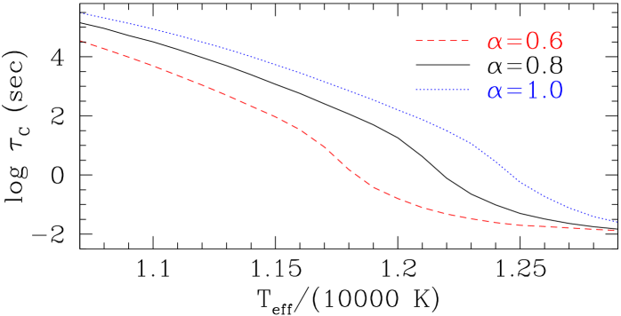
In Figure 1, we show a theoretical calculation of how this timescale $\tau_{C}$ is expected to vary as a function of $T_{\rm eff}$. For a given value of $\alpha$, we see that $\tau_{C}$ changes by approximately a factor of 1000 as the temperature goes from 12000 K (the observed onset of WD pulsations) to 11000 K (the observed disappearance of pulsations). Since a typical pulsator may have excursions in temperature of several hundreds of degrees, we expect $\tau_{C}$ to vary greatly during the pulsations, leading to nonlinear light curves.

Figure 1.: Theoretical calculations of the thermal response timescale of the convection zone, $\tau_{C}$, as a function of $T_{\rm eff}$. The local mixing-length theory of Böhm & Cassinelli (1971) has been used, for the indicated values of $\alpha$.

3. Light Curve Fitting

Using Figure 1 as a guide, we see that although $\tau_{C}$ is a strong function of temperature, its logarithm varies approximately linearly with temperature. Since $\delta F/F=4\,\delta T/T$, $\log\tau_{C}$ is also an approximately linear function of $F$, and since we wish to make as few assumptions about convection as possible, we choose

$$\tau_{C}=\tau_{0}\,e^{a(F_{\rm phot}/F_{0}-1)},$$

where $\tau_{0}$ and $a$ are unknown coefficients and $F_{0}$ is the equilibrium flux.

In addition to the convective parameters $\tau_{0}$ and $a$, we fit the amplitude and phase of the sinusoidal signal at the base of the convection zone (the period is assumed already known from the observations) as well as the inclination angle between the pulsation axis and our line-of-sight.

3.1. The DBV PG1351+049

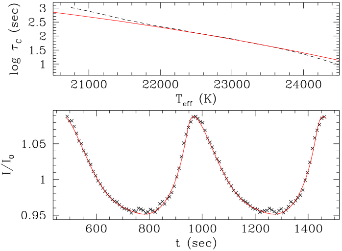
In 1995 data were acquired on the DBV star PG1351+049 as part of a Whole Earth Telescope (WET) campaign (e.g. Winget et al. 1991, 1994). The resulting light curve, which has been folded at the period of the mode, 489.335 s, is shown in the lower panel of Figure 2, where the crosses represent the data and the solid curve is our fit. We note that the fit is very good and reproduces the features in the light curve quite well. In the upper panel we show the convective timescale which we derive from these data (solid curve) as well as one computed using mixing-length theory (dashed curve). The fact that the slopes are similar is encouraging, since the theoretical curve can be moved up or down simply by tuning the value of $\alpha$, while its slope is less sensitive to the choice of $\alpha$.

Figure 2.: A fit to the observed pulse shape of the DBV star PG1351+049.

This star was observed again in May 2004 with the 2.1m telescope at McDonald Observatory. This allows us to make another fit, which provides an important check since we would not expect the parameters characterizing the star itself to have changed, i.e., the average depth of the convection zone, $\tau_{0}$, and the inclination angle, $\theta_{\rm i}$, should be the same, while the amplitude and phase of the mode might very well be different. We summarize these two fits in Table 1: we see that the amplitude of the mode has changed somewhat, but $\theta_{\rm i}$ and $\tau_{0}$ remain the same, i.e., we appear to be looking at the same star.

Table1. Derived parameters for PG1351+049

year	$\tau_{0}$ (sec)	$\theta_{\rm i}$ (deg)	Amp	$\ell$	$m$
1995	99.95	59.4	0.325	1	0
2004	100.83	59.4	0.268	1	0

3.2. The DAV G29-38

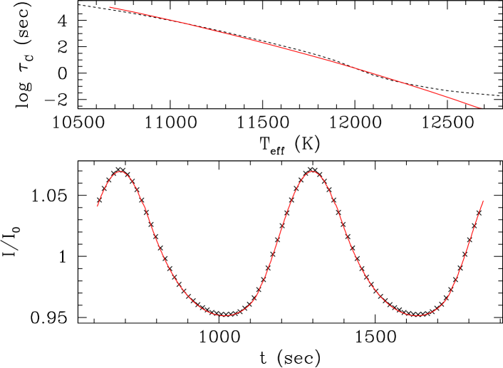
The observations of the DAV G29-38, taken by S. Kleinman in 1988, are displayed as the crosses in the lower panel of Figure 3 (note: the errors on this extremely high signal-to-noise data are actually much smaller than the crosses). Our fit to this data is given by the solid curve, which is nearly indistinguishable from the data except at the maxima and minima, where slight differences can be seen. In the upper panel, we show the derived dependence of $\tau_{C}$ as a function of $T_{\rm eff}$ (solid curve) as well as a theoretical curve computed using mixing-length theory (dashed curve). We see that the slopes of these curves are nearly identical over this region, again implying that we really are measuring something fundamental about this star, and about the physics of convection.

Figure 3.: A fit to the observed pulse shape of the DAV star G29-38.

4. Conclusions

First, the fits we have obtained for the stars PG1351+049 and G29-38 are impressively good, implying that the physical assumptions which have gone into our models are realistic. Second, our results seem to make sense in terms of simple (and naive) theories of convection, and they provide a means of calibrating such models. Third, the fits provide an independent method for determining the $\ell$ and $m$ values of pulsation modes, something which is necessary in order to use asteroseismology to learn about the deep stellar interior.

The ultimate goal of this research is to provide a detailed empirical map of how convection works in these stars, which in terms of their pulsations means mapping how $\tau_{C}$ varies as a function of $T_{\rm eff}$ and $\log g$. Since each pulsator essentially gives us the value of $\tau_{C}$ and its slope at a given $T_{\rm eff}$, by applying this method to stars with temperatures spanning the instability strips of the DAVs and DBVs we can derive this dependence empirically. In the future, this determination will provide an important contact for more sophisticated and physical theories of convection which go beyond mixing-length theory (those without “free parameters”, e.g. Montgomery & Kupka 2004; Kupka & Montgomery 2002) and whose applicability will be to stars throughout the HR diagram.

Acknowledgments.

The author wishes to thank D. O. Gough, D. E. Winget, and D. Koester for useful discussions.

References

- Böhm-Vitense (1958) Böhm-Vitense, E., 1958, Zeitschrift für Astrophysik, 46, 108
- Böhm & Cassinelli (1971) Böhm, K. H., & Cassinelli, J., 1971, A&A, 12, 21
- Bradley & Winget (1994) Bradley, P. A., & Winget, D. E., 1994, ApJ, 430, 850
- Brickhill (1992a) Brickhill, A. J., 1992a, MNRAS, 259, 519
- Brickhill (1992b) Brickhill, A. J., 1992b, MNRAS, 259, 529
- Ising & Koester (2001) Ising, J., & Koester, D., 2001, A&A, 374, 116
- Kupka (1999) Kupka, F., 1999, ApJ, 526, L45
- Kupka & Montgomery (2002) Kupka, F., & Montgomery, M. H., 2002, MNRAS, 330, L6
- Metcalfe (2003) Metcalfe, T. S., 2003, ApJ, 587, L43
- Metcalfe et al. (2004) Metcalfe, T. S., Montgomery, M. H., & Kanaan, A., 2004, ApJ, 605, L133
- Metcalfe et al. (2000) Metcalfe, T. S., Nather, R. E., & Winget, D. E., 2000, ApJ, 545, 974
- Montgomery & Kupka (2004) Montgomery, M. H., & Kupka, F., 2004, MNRAS, 350, 267
- Montgomery & Winget (1999) Montgomery, M. H., & Winget, D. E., 1999, ApJ, 526, 976
- Montgomery et al. (2003) Montgomery, M. H., Metcalfe, T. S., & Winget, D. E., 2003, MNRAS, 344, 657
- Salpeter (1961) Salpeter, E. E., 1961, ApJ, 134, 669
- Winget et al. (1991) Winget, D. E.,Nather, R. E., & Clemens, J. C., 1991, ApJ, 378, 326
- Winget et al. (1994) Winget, D. E.,Nather, R. E., & Clemens, J. C., 1994, ApJ, 430, 839
- Wu (2001) Wu, Y., 2001, MNRAS, 323, 248