Relativistic formulation and reference frame

Abstract

After a short review of experimental foundations of metric theories of gravity, the choice of general relativity as a theory to be used for the routine modeling of Gaia observations is justified. General principles of relativistic modeling of astronomical observations are then sketched and compared to the corresponding Newtonian principles. The fundamental reference system – Barycentric Celestial Reference System, which has been chosen to be the relativistic reference system underlying the future Gaia reference frame is presented. Principal relativistic effects in each constituent of a relativistic model of astronomical observations are briefly elucidated. The structure of a relativistic model of positional observations which can be used as a standard relativistic model for Gaia is sketched. The physical meaning of the Gaia reference frame is discussed. It is discussed also how Gaia observations can be used to verify general relativity.

1 Why relativity?

Reduction scheme of positional observations in Newtonian physics is rather simple. Absolute Euclidean space and absolute time of Newtonian physics lead to the existence of global preferred coordinates: inertial coordinates which are unique up to a constant shift of the origin of the time coordinate, constant rotation of spatial axes and a shift of the origin of spatial coordinates which is at most linear in time. Although already in Newtonian physics one can introduce arbitrary coordinates (e.g., some curvilinear coordinates), the inertial coordinates are certainly preferred since the laws of physics look especially simple when expressed in an inertial reference system. Moreover, observed quantities (distances, directions, etc.) are directly related to those global inertial coordinates.

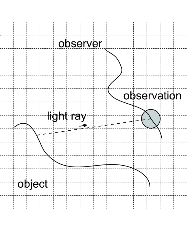
Figure 1: Four parts of an astronomical event from the point of view of Newtonian physics: 1) motion of the observed object; 2) motion of the observer; 3) trajectory of an electromagnetic signal from the observed object to the observer which is tacitly assumed to be a straight line in Newtonian astronomy; 4) the process of observation responsible for Newtonian aberration. The coordinate grid in the background symbolizes a global inertial reference system.

Let us briefly consider the Newtonian scheme of reduction of astronomical observations. Figure 1 sketches the four constituents of an astronomical observation from the point of view of Newtonian physics: (1) motion of the observed object, (2) motion of the observer, (3) propagation of an electromagnetic signal from the object to the observer, and (4) the process of observation. The last two parts can be formulated in a quite simple way in Newtonian physics. It is normally tacitly assumed here that the light rays are straight lines in some inertial coordinates. As for “the process of observation”, it is responsible for the appearance of Newtonian aberration which reflects the difference in observed directions to the source by a moving observer and by an observer at rest relative to the chosen coordinates.

The goal of Newtonian reduction of astronomical observations is to model (to predict) the results of observations performed by a fictitious observer (normally situated at the origin of the chosen reference system, e.g. at the barycenter of the solar system) at some given moment of time. One attempts here to correct for all the effects in observations which are produced by the motion and the position of the real observer (aberration and, e.g., parallax, respectively) and by the motion of the object (proper motion and, possibly, light travel time effects). The structure of a Newtonian reduction scheme does not depend on the goal accuracy of reduction and can be described as follows: (1) aberration, (2) parallax, (3) proper motion and/or light travel time effects. For low accuracies when only linear effects from aberration, parallax and proper motion are of interest, one could apply the corresponding corrections in arbitrary order. On the contrary, for higher accuracies the order of these reductions is important. All parameters of the model, i.e. the coordinates of the observer and the object as function of time, are defined in the chosen inertial reference system. That is, the five standard astrometric parameters of the object (right ascension $\alpha$, declination $\delta$, parallax $\pi$, proper motion in right ascension $\mu_{\alpha}$ and proper motion in declination $\mu_{\delta}$) are also defined in the chosen reference system.

Rapid increase of observational accuracy of astronomical observations has already made indispensable to use general relativity for modeling of the observational data. For many kinds of observations the Newtonian scheme sketched above fails to describe observational data with the required accuracy. In many cases the deviations from the model are several orders of magnitude larger than the accuracy of observations. Examples are astrometric (geodetic) VLBI observations, lunar laser ranging, radar ranging to the planets, experiments with high accuracy clocks, GPS observations. It is also widely known and accepted that the deviations can be eliminated by using Einstein’s general theory of relativity (instead of Newtonian physics) for the modeling of observations.

The accuracy of positional observations to be produced by Gaia is expected to attain 2-3 $\mu$as for the stars with magnitude $V<10$ mag and 10 $\mu$as for the stars of $V=15$ mag. It is clear that not only the largest relativistic effects, but also many additional subtle effects should be taken into account to attain that accuracy. It is also quite clear that relativistic effects cannot be considered as small corrections to a Newtonian model as has been often done earlier when the accuracy was not so high. The whole model should be formulated in a language compatible with general relativity. In such a relativistic framework many Newtonian concepts must be abandoned and the meaning of astrometric parameters such as position, parallax and proper motion of a star should be redefined.

2 Experimental foundations of general relativity

Einstein’s general relativity is by no means the only possible theory of gravity. However, it seems to be the simplest theory among the theories successfully passing all available observational tests. Let us briefly review the experimental foundations of general relativity. A detailed review of the modern experimental foundations of gravitational physics can be found in Will (2001).

2.1 Einstein Equivalence Principle

The basic principle of the theory is called Einstein Equivalence Principle. This principle consists of the following three parts:

(1) The Weak Equivalence Principle stating that the masses on the both sides of the Newtonian gravitational law

$$m_{iner}\,\ddot{r}^{i}=-G\,m_{grav}\,M\,r^{i}\,/\,r^{3}$$

exactly coincide $m_{iner}\equiv m_{grav}$ for all bodies (actually, this is equivalent to the claim that $G$ is a constant and its value is independent of the choice of the bodies with which we measure it). The Weak Equivalence Principle has been tested in many different experiments with a precision of $|\delta m|/m<4\cdot 10^{-13}$.

(2) Local Lorentz invariance stating that the outcome of any local non-gravitational experiment is independent of the velocity of the freely-falling test laboratory (reference frame) where it is performed. This is equivalent to the principal postulate of special relativity theory which states that the light velocity in vacuum $c$ is constant in any inertial reference system. This has been tested at a level of $\sim 10^{-21}$.

(3) Local positional invariance which states that the outcome of any local non-gravitational experiment is independent of where and when in the universe it is performed. A part of local positional invariance can be tested by measuring of the gravitational red shift (e.g., of the clock frequency)

$$\Delta\nu\,/\,\nu=(1+\alpha)\,c^{-2}\,\Delta U,$$

where $\alpha=0$ in general relativity. A number of different experiments has proved that $|\alpha|<2\cdot 10^{-4}$. Another part of local positional invariance (independence of “position” in time) can be tested by looking for possible time-dependencies of fundamental (non-gravitational) constants. Different kinds of experimental data show tight constrains on possible time-dependence of the constants (e.g., the fine structure constant should be constant at a precision of $\sim 10^{-6}$ over Hubble time of 13 billion years).

Table 1: Most important post-Newtonian tests of general relativity

observational data	relativistic effect	possible deviation	reference
		from general relativity
VLBI	differential Shapiro delay	$\pm 0.0003$	Eubanks et al. (1997)
HIPPARCOS	light deflection	$\pm 0.003$	Froeschlé et al. (1997)
Viking radar ranging	Shapiro delay	$\pm 0.002$	Reasenberg et al. (1979)
Cassini radar ranging	Shapiro delay	$\pm 0.000023$	Bertotti et al. (2003)
planetary observations	perihelion advance	$\pm 0.0002$	Pitjeva (2001)
Lunar laser ranging	Nordtvedt effect	$\pm 0.001$	Williams et al. (1996)
Lunar laser ranging	geodetic precession	$\pm 0.001$	Williams et al. (1996)

2.2 Testing metric theories of gravity

One can argue that if the Einstein Equivalence Principle is valid the gravity can be interpreted as an effect of curved spacetime. However, the Einstein Equivalence Principle does not necessarily imply general relativity. There exists a class of alternative theories of gravity compatible with that Principle. These theories are called metric theories of gravity. In order to test the principal observable effects of metric theories of gravity a special scheme called Parametrized Post-Newtonian (PPN) formalism has been proposed (Will 1993). The scheme involves up to 10 numerical parameters which have different values in different theories and which can be fitted from observations. The most important PPN parameters are $\gamma$ and $\beta$. Results of data processing with a PPN reduction model incolve a set of constraints on the PPN parameters. Alternatively, the results can be interpreted as boundaries on possible deviations from general relativity. The most important experimental results in this second interpretation are summarized in Table 1.

An additional test of general relativity is the search for possible time-dependence of Newtonian gravitational constant $G$. This can be done by looking for secular changes in semi-major axes of solar system planets (especially, Mercury, Venus, Earth and Mars) as well as from pulsar timing of double pulsars. The most stringent estimate here is $|\dot{G}/G|<10^{-13}$ per year (Pitjeva 2001). General relativity predicts that $G$ is time-independent. One more argument in favor of general relativity is the well-known indirect evidence for gravitational radiation in the double pulsar timing data. Gravitational radiation is strong-field regime phenomenon which is beyond the scope of the PPN formalism.

All this shows that one can be “reasonably confident” about the correctness of general relativity, and that general relativity can be used as “standard” theory. Nevertheless, it is still very important to test general relativity further. This will be discussed below in Section 6.

3 Relativistic modeling of astronomical observations

Let us now outline general principles of relativistic modeling of astronomical observations. It is interesting that in spite of a deep conceptual difference between Newtonian physics and general relativity, the structure of the reduction scheme changes, in principle, only in one point: light rays are no longer straight lines and should be carefully modeled. Figure 2 shows the four constituents of an astronomical observation in the relativistic framework. In curved spacetime there is no preferred coordinates where the laws of physics would have substantial simpler form than in other coordinates. Therefore, any reference system covering the spacetime region under study can be used. Instead of Newtonian inertial coordinates one has to choose some reference system in curved spacetime which is sketched symbolically on Figure 2 as a grid of curved coordinates.

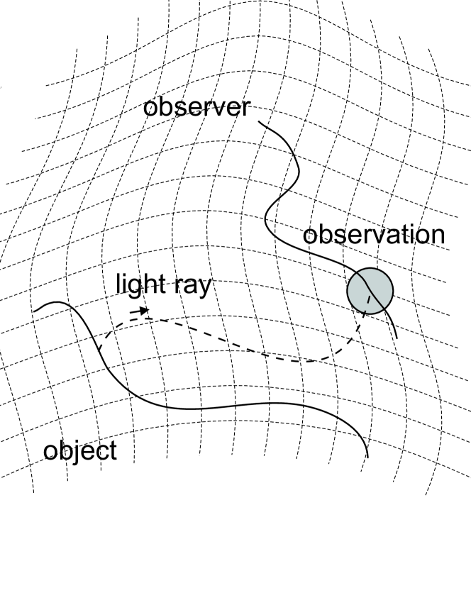
Figure 2: Four parts of an astronomical event from the point of view of relativistic physics: 1) motion of the observed object; 2) motion of the observer; 3) trajectory of an electromagnetic signal from the observed object to the observer which represents a geodetic line (i.e. a “curved” line) in the chosen reference system; 4) the process of observation. The grid of curved coordinates in the background symbolizes the chosen relativistic reference system.

3.1 General scheme of relativistic modeling

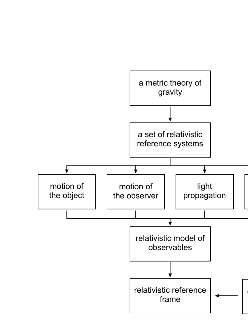
Figure 3: General principles of relativistic modeling of astronomical observations (see text for further explanations).

General scheme of relativistic modeling is presented on Figure 3. Starting from general theory of relativity, any other metric theory of gravity or the PPN formalism one should define at least one relativistic 4-dimensional reference system covering the region of space-time where all the processes constituting particular kind of astronomical observations are located. Each of four constituents of an astronomical observation should be modeled in the relativistic framework. The equations of motion of both the observed object and the observer relative to the chosen reference system should be derived and a method to solve these equations should be found. The equations of light propagation relative to the chosen reference system should be derived and a way to solve them should be found. The equations of motion of the object and the observer and the equations of light propagation enable one to compute positions and velocities of the object, observer and the photon (light ray) with respect to that particular reference system at a given moment of the coordinate time, provided that the positions and velocities at some initial epoch are known. However, the positions and velocities calculated in this way obviously depend on the reference system, that is on the preferences of the person who writes down the equations. On the other hand, the results of observations cannot depend on the choice of the reference system. Therefore, it is clear that one more step of the modeling is needed: a relativistic description of the process of observation. This part of the model allows one to compute a coordinate-independent theoretical prediction of observables starting from the coordinate-dependent quantities mentioned above.

These four components can now be combined into relativistic models of observables. The models give an expression for relevant observables as a function of a set of parameters. These parameters can then be fitted to observational data using some kind of parameter estimation scheme. The sets of certain estimated parameters appearing in the relativistic models of observables represent astronomical reference frames (see Section 5). It is important to understand at this point that the relativistic models contain some parameters which are defined only in the chosen reference system(s) and are thus coordinate-dependent. For example, position and velocity of the observed object are clearly coordinate-dependent.

3.2 The Barycentric Celestial Reference System

From the physical point of view any reference system covering the region of space-time under consideration can be used to describe physical phenomena within that region. In this sense we are free to choose the reference system to be used to model the observations. However, reference systems, in which mathematical description of physical laws is in one sense or another simpler than in some other reference systems, are more convenient for practical calculations. Therefore, one can use the freedom to choose the reference system to make the parametrization as convenient and reasonable as possible.

Two Working Groups on relativity in astrometry, celestial mechanics and metrology established 1997 by the International Astronomical Union (IAU) and Bureau International des Poids and Mesure (BIPM) have come to the conclusion that the most convenient relativistic reference system for the applications in astrometry, solar system dynamics, and time keeping and dissemination is defined by the following metric tensor (Soffel et al. 2003):

$$g_{00} = -1+{2w\over c^{2}}-{2w^{2}\over c^{4}}+{\cal O}(c^{-5}),$$

$$g_{0i} = -{4\over c^{3}}w^{i}+{\cal O}(c^{-5}),$$

$$g_{ij} = \delta_{ij}\left(1+{2\over c^{2}}w\right)+{\cal O}(c^{-4})\,$$ (1)

with the post-Newtonian potentials $w$ and $w^{i}$ defined by

$$w(t,\mbox{\boldmath$x$}) = G\int d^{3}x^{\prime}\,{\sigma(t,\mbox{\boldmath$x$}^{\prime})\over|\mbox{\boldmath$x$}-\mbox{\boldmath$x$}^{\prime}|}$$ (2)

$$+{1\over 2c^{2}}G{\partial^{2}\over\partial t^{2}}\int d^{3}x^{\prime}\,\sigma(t,\mbox{\boldmath$x$}^{\prime})|\mbox{\boldmath$x$}-\mbox{\boldmath$x$}^{\prime}|\,,$$

$$w^{i}(t,\mbox{\boldmath$x$}) = G\int d^{3}x^{\prime}{\sigma^{i}(t,\mbox{\boldmath$x$}^{\prime})\over|\mbox{\boldmath$x$}-\mbox{\boldmath$x$}^{\prime}|}\,,$$ (3)

$\sigma$ and $\sigma^{i}$ being related to the components of the energy-momentum tensor $T^{\alpha\beta}$:

$$\sigma={1\over c^{2}}\left(T^{00}+T^{ss}\right),\quad\sigma^{i}={1\over c}\ T^{0i}\,.$$ (4)

The origin of spatial coordinates of this reference system is chosen to coincide with the barycenter of the solar system. The reference system defined in this way is called Barycentric Celestial Reference System (BCRS). The BCRS has been explicitly recommended by the IAU for the modeling of high accuracy astronomical observations (IAU 2001; Rickman 2001; Soffel et al. 2003). For the moment the BCRS is a post-Newtonian reference system with higher order terms (post-post-Newtonian terms, etc.) neglected in the metric tensor (3.2). The reason for that is that the post-Newtonian approximation is sufficient to model any observations in forseeable future (including microarcsecond astrometry as long as the observations are made further than about one degree from the Sun). Post-post-Newtonian terms can be added to the metric tensor as soon as they are necessary for some applications. The word “celestial” in the name of BCRS is used to underline that the BCRS do not rotate with the Earth and that remote sources do not move relative to the BCRS in some averaged sense. The second reference system deined by the same IAU resolutions (Rickman 2001) is the Geocentric Celestial Reference System (GCRS). This reference system is only marginally important for Gaia (mostly for modeling of orbit tracking data and relating the Gaia onboard clock to TAI (Klioner 2003a)) and will not be discussed here. The PPN version of the BCRS valid for certain class of metric theories of gravity can be found in Klioner & Soffel (2000) and Will (1993).

The BCRS will be also used for the modeling of Gaia observations. This is a reference system underlying the resulting Gaia catalogue (see Section 5 below). The coordinate time of the BCRS is called Barycentric Coordinate Time (TCB). The TCB will be used to parametrize the Gaia catalogue.

3.3 Motion of the objects and the observer

Typically, for objects situated in the solar system (asteroids, planets, space vehicles) the equations of motion are ordinary differential equations of second order and numerical integration with suitable initial or boundary conditions can be used to solve them. For objects outside of the solar system one use often simple models like uniform and rectilinear motion in space or more complicated ones, e.g., for binary stars. In any case one should understand that in the relativistic framework all these ad hoc models give positions and velocities of observed objects in the chosen relativistic reference system.

The principal relativistic effects in the translational motion of bodies in the solar system (including Gaia satellite, asteroids, etc.) are contained in the so-called Einstein-Infeld-Hoffmann (EIH) equations of motion of $N$ gravitating bodies, whose gravitational fields can be described by their masses $M_{A}$ only:

$$\ddot{\mbox{\boldmath$x$}}_{A} = -\sum_{B\neq A}G\,M_{B}\,{\mbox{\boldmath$x$}_{A}-\mbox{\boldmath$x$}_{B}\over|\mbox{\boldmath$x$}_{A}-\mbox{\boldmath$x$}_{B}|^{3}}$$ (5)

$$+{1\over c^{2}}\,{\bf F}_{pN}(M_{B},\mbox{\boldmath$x$}_{B},\dot{\mbox{\boldmath$x$}}_{B})+{\cal O}(c^{-4}).$$

The Newtonian part of these equations (shown explicitly above) follows from the term of order $c^{-2}$ in $g_{00}$. The relativistic terms require all other terms in the BCRS metric tensor specified above. Various parts of these equations represent: (1) relativistic perihelion advance ($\sim$43 ^′′/cty for Mercury, $\sim$10 ^′′/cty for Icarus, etc.); (2) geodetic precession ($\sim$2 ^′′/cty for Lunar orbit); (3) various periodic relativistic effects (important mostly for LLR and binary pulsar timing observations). Further effects not contained in the EIH equations are the effects due to rotation of the bodies (Lense-Thirring or gravitomagnetic effects) and those due to non-sphericity of the gravitating bodies. These additional effects are marginal for the current accuracy of LLR and SLR, but negligible for Gaia. In case of Gaia satellite one should use a slightly simplified version of the EIH equations since the influence of the mass of the satellite on the motion of other gravitating bodies can be neglected.

The BCRS metric tensor allows one also to derive the equations of rotational motion of an extended body. These equations will not be discussed here, since they are not important for Gaia.

3.4 Light propagation

In any metric theory of gravity the equations of light propagation coincide with the equations of geodetic lines in the chosen reference system. The latter are ordinary differential equations of second order. These equations could also be solved by numerical integrations, but normally one prefer to use some approximate analytical solutions. Only in some special (normally, highly symmetrical) cases like Schwarzschild metric exact analytical solutions are known. Anyway, an appropriate way to solve the equations of light propagation should be found.

The structure of the BCRS equations of light propagation can be written as follows

$$\mbox{\boldmath$x$}(t)=\mbox{\boldmath$x$}_{0} + c\,\mbox{\boldmath$\sigma$}\,(t-t_{0})+c^{-2}\,{\bf S}_{pN}(t)$$ (6)

$$+ c^{-3}\,{\bf S}_{1.5pN}(t),$$

where $\mbox{\boldmath$x$}_{0}$ and $\sigma$ are the parameters of Newtonian straight line, ${\bf S}_{pN}$ are the post-Newtonian terms, and ${\bf S}_{1.5pN}$ are the additional effects induced by the motion of gravitating matter (i.e., by translational and rotational motion of gravitating bodies). The terms of order of $c^{-2}$ in both $g_{00}$ and $g_{ij}$ are required to derive ${\bf S}_{pN}(t)$, and the terms $c^{-3}$ in $g_{0i}$ are needed for ${\bf S}_{1.5pN}$. The next order effects, the so-called post-post-Newtonian effects, would require terms of order of $c^{-4}$ in both $g_{00}$ and $g_{ij}$ (the $c^{-4}$ terms in $g_{ij}$ are not in the current definition of the BCRS metric tensor). The principle observable effects in the light propagation are (1) the gravitational light deflection (amounting to $1.75{\hbox{${}^{\prime\prime}$}}$ for a light ray grazing the Sun) and (2) the gravitational signal retardation (the Shapiro effect; this effect amounts to $\sim 240$ $\mu$s for the radar ranging of Venus in upper conjunction).

3.5 Conversion to observables: proper direction

As mentioned above the conversion the coordinate-dependent quantities into coordinate-independent observables is an important part of relativistic modeling. From the mathematically point of view the coordinate-independent quantities are scalars. Special mathematical techniques are known to perform the suitable conversion in each particular case. One of the most important application of this conversion procedure is a conversion of the coordinate direction $n$ into the source into the corresponding observable direction $s$. The observable direction is often called “proper direction” in gravitational physics. Proper direction is a direction relative to the proper reference frame of the observer (see Section 5 about the difference of the concept of “reference frame” in astronomy and gravitational physics). A proper reference frame is a mathematical model of an ideal clock and three orthogonal rigid rods which the observer uses to measure time intervals, distances and directions in his vicinity. In special theory of relativity the proper reference frame of an observer is related to some inertial reference system by a Lorentz transformation. It is therefore, sufficient to use Lorentz transformations to convert $n$ into $s$. The parameter of the Lorentz transformation in this case coincides with the velocity of the observer relative to the chosen reference system. In general relativity it is also sufficient to use Lorentz transformations, but the parameter $\nu$ of the transformations should be related to the BCRS velocity of the observer as

$$\mbox{\boldmath$\nu$}=\dot{\mbox{\boldmath$x$}}_{o}\,\left(1+{2\over c^{2}}w(t,\mbox{\boldmath$x$}_{o})\right)+{\cal O}(c^{-4}),$$ (7)

where $\mbox{\boldmath$x$}_{o}$ and $\dot{\mbox{\boldmath$x$}}_{o}$ are the BCRS positions and velocity of the observer, respectively. A detailed discussion of this conversion and comparison of different approaches can be found in Klioner (2003b). The relativistic terms in (7) are derived from the $c^{-2}$ terms in $g_{00}$ and $g_{ij}$ of the BCRS metric tensor. The difference between $n$ and $s$ can be called relativistic aberration. The difference between the Newtonian aberration and the relativistic one may amount to several milliarcsecond for Gaia observations.

3.6 Conversion to observables: proper time

Another important case is the conversion of intervals of the coordinate time $t$ into the corresponding intervals of the proper time $\tau$ of the observer. The general form of this conversion reads

$$d\tau\,/\,dt=1+c^{-2}\,A_{pN}+c^{-4}\,A_{ppN}+{\cal O}(c^{-5}),$$ (8)

where $A_{pN}$ and $A_{ppN}$ are the post-Newtonian and post-post-Newtonian terms, respectively. Explicit form of these two functions depends on the metric tensor: in order to compute for $A_{pN}$ the $c^{-2}$ terms in $g_{00}$ are needed, while the $c^{-4}$ terms in $g_{00}$, the $c^{-3}$ terms in $g_{0i}$, and the $c^{-2}$ ones in $g_{ij}$ are required to compute $A_{ppN}$. Typically in the Solar system and in particular for Gaia onboard clocks $|c^{-2}\,A_{pN}|\sim 10^{-8}$ and $|c^{-4}\,A_{ppN}|\sim 10^{-16}$.

4 Relativity for Gaia

Now, having all these theoretical tools one can formulate the relativistic model for Gaia. The relativistic model for Gaia is well documented (Klioner 2003a), so that we just outline the overall structure of the model here.

4.1 Structure of the standard relativistic model

Figure 4: Five principal vectors used in the model (see text for explanations).

The model consists essentially in subsequent transformations between 5 following vectors (Figure 4):

a) $s$ is the unit observed direction (the word “unit” means here and below that the formally Euclidean scalar product $\mbox{\boldmath$s$}\,\cdot\,\mbox{\boldmath$s$}=s^{i}\,s^{i}$ is equal to unity),

b) $n$ is the unit vector tangential to the light ray at the moment of observation,

c) $\sigma$ is the unit vector tangential to the light ray at $t=-\infty$,

d) $k$ is the unit coordinate vector from the source to the observer,

e) $l$ is the unit vector from the barycenter of the Solar system to the source.

Note that the last four vectors should be interpreted as sets of three numbers characterizing the position of the source with respect to the BCRS. Vector $s$ represents components of the observed direction relative to the local proper reference system of the satellite. All these vectors would change their numerical values if some other relativistic reference system is used instead of the BCRS. The model consists then in a sequence of transformations between these vectors as shown on Figure 5. The physical meaning of each transformation can be summarized as follows (the numbering here coincides with the numbering on Figure 5):

remote sources:  $\mbox{\boldmath$s$}\ {\mathop{\vtop{\halign{#\cr$\hfil\displaystyle{\longleftrightarrow}\hfil$\crcr\kern 0.1pt\nointerlineskip\cr\kern 0.1pt\cr}}}\limits^{\scriptscriptstyle(1)}}{}\ \mbox{\boldmath$n$}\ {\mathop{\vtop{\halign{#\cr$\hfil\displaystyle{\longleftrightarrow}\hfil$\crcr\kern 0.1pt\nointerlineskip\cr\kern 0.1pt\cr}}}\limits^{\scriptscriptstyle(2)}}{}\ \mbox{\boldmath$\sigma$}\ {\mathop{\vtop{\halign{#\cr$\hfil\displaystyle{\longleftrightarrow}\hfil$\crcr\kern 0.1pt\nointerlineskip\cr\kern 0.1pt\cr}}}\limits^{\scriptscriptstyle(3)}}{}\ \mbox{\boldmath$k$}\ {\mathop{\vtop{\halign{#\cr$\hfil\displaystyle{\longleftrightarrow}\hfil$\crcr\kern 0.1pt\nointerlineskip\cr\kern 0.1pt\cr}}}\limits^{\scriptscriptstyle(4)}}{}\ \mbox{\boldmath$l$},\pi\ {\mathop{\vtop{\halign{#\cr$\hfil\displaystyle{\longleftrightarrow}\hfil$\crcr\kern 0.1pt\nointerlineskip\cr\kern 0.1pt\cr}}}\limits^{\scriptscriptstyle(5)}}{}\ \mbox{\boldmath$l$}(t_{0}),\pi(t_{0}),\mbox{\boldmath$\mu$}(t_{0}),\dots$

solar system objects: $\mbox{\boldmath$s$}\ {\mathop{\vtop{\halign{#\cr$\hfil\displaystyle{\longleftrightarrow}\hfil$\crcr\kern 0.1pt\nointerlineskip\cr\kern 0.1pt\cr}}}\limits^{\scriptscriptstyle(1)}}{}\ \mbox{\boldmath$n$}\ {\mathop{\vtop{\halign{#\cr$\hfil\displaystyle{\longleftrightarrow}\hfil$\crcr\kern 0.1pt\nointerlineskip\cr\kern 0.1pt\cr}}}\limits^{\scriptscriptstyle(2,3)}}{}\ \mbox{\boldmath$k$}\ {\mathop{\vtop{\halign{#\cr$\hfil\displaystyle{\longleftrightarrow}\hfil$\crcr\kern 0.1pt\nointerlineskip\cr\kern 0.1pt\cr}}}\limits^{\scriptscriptstyle(6)}}{}\ {\rm orbit}$

Figure 5: Transformation sequences (see text for explanations).

(1) aberration (effects vanishing together with the barycentric velocity of the observer): this step converts the observed direction to the source $s$ into the unit BCRS coordinate velocity of the light ray $n$ at the point of observation;

(2) gravitational light deflection for the source at infinity: this step converts $n$ into the unit direction of propagation $\sigma$ of the light ray infinitely far from the solar system at $t\to-\infty$;

(3) coupling of finite distance to the source and the gravitational light deflection in the gravitational field of the solar system: this step converts $\sigma$ into a unit BCRS coordinate direction $k$ going from the source to the observer;

(4) parallax: this step converts $k$ into a unit BCRS direction $l$ going from the barycenter of the Solar system to the source;

(5) proper motion, etc: this step provides a reasonable parametrization of the time dependence of $l$ (and, possibly, of the parallax $\pi$) caused by the motion of the source relative to the barycenter of the Solar system;

(6) orbit determination process.

These transformations have already been discussed in full detail (Klioner 2003a; Klioner & Peip 2003; Klioner 2003b). Let us only mention the following. The most complicated part of the model is the light deflection model where the effects of (1) monopole fields of all major solar system bodies, (2) quadrupole fields of the giant planets, and (3) gravitomagnetic fields due to translational motion of all major bodies should be taken into account in order to attain the accuracy of 1 $\mu$as. Moreover, each body with a mean density $\rho$ and radius $R\geq(\rho/1\ {\rm g/cm}^{3})^{-1/2}\times 650$ km produces a light deflection of at least 1 $\mu$as. Therefore, a few tens of minor bodies (mainly, satellites of the giant planets) should also be taken into account in certain rare cases (Klioner 2003a). The parametrization of time dependence of $l$ in the relativistic framework looks exactly the same as in the Newtonian case. The only difference is that all vectors and parameters here (parallax, proper motion, etc.) are coordinate quantities defined in the BCRS.

4.2 Implementation of the model

An ANSI C code has been written to implement the relativistic model in its full complexity (Klioner & Blankenburg 2003; Klioner 2003b). The model has been implemented in two modes: predictor mode and corrector mode. Predictor mode implements the standard way of astrometric reductions when the observed direction to the source is predicted starting from some a priori catalogue parameters (coordinates, proper motion, parallax, etc.) of that source. The catalogue is supposed to be improved later by fitting the parameters to the whole set of data. Corrector mode implements the reductions in the opposite direction, that is, the momentary barycentric direction to the source is restored from the observed direction as good as possible. The code does not contain any attempt to restore parallaxes and proper motions, or orbits of the sources: the model can only be applied separately for each individual observation.

Both modes are implemented both for solar system objects and for remote sources situated outside of the solar system. The principal difference between remote sources and solar system sources lies in the treatment of the light propagation: an initial value solution of the corresponding differential equations is used in the former case, while in the latter case two point boundary value problem should be solved. Although analytical approximations are used in both cases, a rather time-consuming numerical inversion process is used for solar system sources in the predictor mode in order to attain the goal accuracy of 1 $\mu$as. The corresponding refinement of the model aimed at direct analytical solution for this case is underway (Klioner & Blankenburg 2004).

For remote sources the corrector and predictor modes being implemented independently of each other must give exactly the opposite transformations. This was used to massively test the implementation (Klioner & Blankenburg 2003). The situation is different for solar system objects. Here for the corrector mode, it is statistically better to calculate the gravitational light deflection as if the body were a remote source, even if it is known a priori that the source is a solar system body (but it is not known how far the body is, otherwise at least a preliminary orbit is known and one should better use the predictor mode).

The implementation was conceived to be as flexible as possible. Internal parameters allow one to select the type of arithmetic to be used (to test possible numerical instabilities), to change easily any of the physical, mathematical and astronomical constants used in the model (including switching between several available planetary ephemerides), to switch on and off each individual effect. Both predictor and corrector mode routines have a goal accuracy parameter, which is used together with some a priori criteria to decide which effects should be computed in each particular case. The latter feature allows one to speed up the calculations substantially if a lower accuracy is sufficient (e.g. the source brightness information can be used to meet the Gaia observational accuracy for fainter objects).

The implementation has been used in massive numerical tests aimed at identifying possible inconsistencies or numerical instabilities as well as points of critical numerical performance. The implementation was used also to test another simplified model implementation used in the GDAAS (Anglada-Escudé et al. 2003). The implementation of the full model will be further supported and optimized.

4.3 Beyond the standard relativistic model

The model described above is constructed under assumption that the solar system is isolated. This means that any influence of gravitational fields generated outside of the solar system are ignored in the model. For the majority of the sources the external field can indeed be fully neglected, but there are a number of cases when the external gravitational fields produce observable effects. Several authors have discussed these additional effects in detail (see, e.g., Klioner (2003a) and Kopeikin & Gwinn (2000)). Let us briefly list here the main effects of this kind:

(1) Gravitational light deflection caused by the masses situated outside of the solar system: (a) weak microlensing on the stars of the Galaxy (Belokurov & Evans 2002), (b) lensing on gravitational waves (both primordial ones and those from compact sources), (c) lensing of the companions of edge-on binary systems.

(2) Cosmological effects.

(3) More complicated models for the motions of observed objects in the BCRS are necessary for the case of binary stars, etc.

Note that all these effects can be easily taken into account by a simple additive extension of the standard model since at the required accuracy the external gravitational fields can be linearly superimposed on the solar system gravitational field. The only exception could be the effects of cosmological background, but a preliminary study by Klioner & Soffel (2004) shows that even here the coupling of the local solar system fields and the external ones can be neglected.

5 Gaia reference frame

It is important to remember that all astrometric parameters of sources obtained from Gaia observations will be defined in the BCRS coordinates: positions, proper motions, parallaxes, radial velocities, orbits of minor planets, binaries, etc. All these parameters will represent the Gaia reference frame, which is a materialization of the BCRS. The Gaia reference frame is, so to say, a model of the universe in the BCRS. Thus, the goal of astrometry in the relativistic framework is not to find “the” barycentric inertial reference system, which is unique in Newtonian formulation, but to find a materialization of some chosen relativistic reference system.

Let us note here that the meaning of words “reference system” and “reference frame” in relativistic astronomy is different from the meaning normally used in gravitational physics. Reference system is a purely mathematical construction (a chart) giving “names” to space-time events. A reference frame is, in contrast, some materialization (realization) of a reference system. In astronomy the materialization is normally given in a form of a catalogue (or ephemeris) containing positions of some celestial objects relative to the selected reference system. Any astronomical reference frame (a catalogue, an ephemeris, etc) is defined only through the reference system(s) used to construct physical models of observations.

6 Gaia for Relativity

Using general relativity for the standard reduction model does not mean that Gaia data should not be used to test general relativity itself. On the contrary, testing relativity is one of the exciting goals of the mission. Gaia will certainly deliver an estimate of the PPN parameter $\gamma$, appearing mainly in the magnitude of the light deflection effects, with an unprecedented accuracy of $\sim 5\times 10^{-7}$. However, it is by no means the only way Gaia will improve our knowledge of gravitational physics. Gravitational light deflection could be tested in a much more profound way with the Gaia data Gaia. It will be certainly possible to look for terms with totally different dependence on the angular distance to the deflecting body. In this sense one should be able to get first experimental estimates of higher-order effects. Also the PPN parameter $\beta$, appearing in the equations of motion of solar system bodies, will be determined with an accuracy of $\sim 10^{-4}$ (Hestrofer & Berthier 2004) which is comparable with the current accuracy from the planetary fits (Pitjeva 2001). A simultaneous fit with the planetary data could further improve the accuracy. Special data processing of observations close to Jupiter and Saturn (which should be dropped from the global absolute solution since the positions of those planets are not known with an accuracy necessary to predict the light deflection at the level of 1 $\mu$as) will allow to test subtle relativistic effects caused by translational motion of the planets and by their quadrupole gravitational fields (see Crosta & Mignard (2004) for a preliminary study of the second of these possibilities). A number of cosmological tests (upper estimates of parallaxes of quasars, apparent proper motions of quasars, possible traces of low-frequency gravitational waves in those proper motions, direct measurement of the acceleration of the solar system relative to quasars, etc.) will also have a big impact on our knowledge. A lot of work is still necessary to understand how to use the full potential of the huge amount of observation data Gaia will deliver to us in the most efficient and useful way.

References

- Anglada-Escudé et al. (2003) Anglada-Escudé, G., Torra, J., Masana, E., Luri, X., 2004, this volume
- Bertotti et al. (2003) Bertotti, B., Iess, L, Tortora, P. 2003, Nature, 425, 374
- Belokurov & Evans (2002) Belokurov, V.A., & Evans, N.W. 2002, MNRAS, 331, 649
- Crosta & Mignard (2004) Crosta, M.T., Mignard, F. 2004, this volume
- Eubanks et al. (1997) Eubanks, T. M. et al. 1997 In: Proc. of The Joint APS/AAPT 1997 Meeting, 18-21 April 1997, Washington D.C.
- Froeschlé et al. (1997) Froeschlé, M., Mignard, F., & Arenou, F. 1997, in Proceedings of the ESA Symposium “Hipparcos - Venice 97”, ESA SP-402, 49
- Hestrofer & Berthier (2004) Hestrofer, D., Berthier, J. 2004, this volume
- IAU (2001) IAU 2001, Information Bulletin, 88 (errata in IAU Information Bulletin, 89)
- Klioner (2003a) Klioner, S.A., 2003a, AJ, 125, 1580
- Klioner (2003b) Klioner, S.A., 2003b, Phys. Rev. D, 69, 124001
- Klioner (2003b) Klioner, S.A., 2003c, Technical report on the implementation of the GAIA relativistic model, Amendment for version 1.0g, available from the GAIA document archive http://astro.estec.esa.nl/llink/livelink
- Klioner & Blankenburg (2003) Klioner, S.A., & Blankenburg, R. 2003, Technical report on the implementation of the GAIA relativistic model, available from the GAIA document archive http://astro.estec.esa.nl/llink/livelink
- Klioner & Blankenburg (2004) Klioner, S.A., & Blankenburg, R. 2004, On the second-order effects in two point boundary value problem in the light propagation, under preparation
- Klioner & Kopeikin (1992) Klioner S.A., & Kopeikin, S.M. 1992, AJ, 104, 897
- Klioner & Soffel (2000) Klioner, S.A., & Soffel, M.H. 2000, Phys. Rev. D, 62, ID 024019
- Klioner & Soffel (2004) Klioner, S.A., & Soffel, M.H. 2004, this volume
- Klioner & Peip (2003) Klioner, S.A., Peip, M. 2003, A&A, 410, 1063
- Kopeikin & Gwinn (2000) Kopeikin, S.M., & Gwinn, C. 2000, in Towards Models and Constants for Sub-Microarcsecond Astrometry, ed. K.J. Johnston, D.D. McCarthy, B.J. Luzum, & G.H. Kaplan (Washington: US Naval Observatory), 303
- Soffel et al. (2003) Soffel, M. et al. 2003, AJ, 126, 2687
- Pitjeva (2001) Pitjeva, E. 2001, A&A, 371, 760
- Reasenberg et al. (1979) Reasenberg, R. D. et al. 1979, ApJ, 234, L219
- Rickman (2001) Rickman, H. 2001, Reports on Astronomy, Trans. IAU, XXIV B
- Will (1993) Will, C. M. 1993, Theory and experiment in gravitational physics (Cambridge: Cambridge University Press)
- Will (2001) Will, C.M., 2001, The Confrontation between General Relativity and Experiment”, Living Rev. Relativity, 4, 4. [Online Article]: cited on 12 November 2004, http://www.livingreviews.org/Articles/Volume4/2001-4will/.
- Williams et al. (1996) Williams, J.G., Newhall, X.X., & Dickey, J.O. 1996, Phys. Rev. D, 53, 6730