Positron annihilation spectrum from the Galactic Center region observed by SPI/INTEGRAL

Abstract

The electron-positron annihilation spectrum observed by SPI/INTEGRAL during deep Galactic Center region exposure is reported. The line energy (510.954$\pm$0.075 keV) is consistent with the unshifted annihilation line. The width of the annihilation line is 2.37$\pm$0.25 keV (FWHM), while the strength of the ortho-positronium continuum suggests that the dominant fraction of positrons (94$\pm$6%) form positronium before annihilation. Compared to the previous missions these deep INTEGRAL observations provide the most stringent constraints on the line energy and width.

Under the assumption of an annihilation in a single-phase medium these spectral parameters can be explained by a warm $T_{e}\sim 7000-4~{}10^{4}$ K gas with the degree of ionization larger than a few $10^{-2}$. One of the wide-spread ISM phases - warm ($T_{e}\sim 8000$ K) and weakly ionized (degree of ionization $\sim$ 0.1) medium satisfies these criteria. Other single-phase solutions are also formally allowed by the data (e.g. cold, but substantially ionized ISM), but such solutions are believed to be astrophysically unimportant.

The observed spectrum can also be explained by the annihilation in a multi-phase ISM. The fraction of positrons annihilating in a very hot ($T_{e}\geq 10^{6}$ K) phase is constrained to be less than $\sim$8%. Neither a moderately hot ($T_{e}\geq 10^{5}$ K) ionized medium nor a very cold ($T_{e}\leq 10^{3}$ K) neutral medium can make a dominant contribution to the observed annihilation spectrum. However, a combination of cold/neutral, warm/neutral and warm/ionized phases in comparable proportions could also be consistent with the data.

1 Introduction

The annihilation line of positrons at 511 keV is the brightest gamma-ray line in the Galaxy. First observed with a NaI scintillator as a $\sim$ 476 keV line coming from the Galactic Center (GC) region (Johnson, Harnden & Haymes, 1972; Johnston & Haymes, 1973), it was subsequently unambiguously identified with a narrow ($FWHM<3.2$ keV)   $e^{+}e^{-}$ annihilation line using germanium detectors (Leventhal, MacCallum, Stang, 1978). Since then many balloon flights and several space missions have measured the spatial distribution and spectral properties of the line. A summary of the high energy resolution observations of the 511 keV line prior to INTEGRAL and the first SPI/INTEGRAL results can be found in Jean et al. (2003) and Teegarden et al. (2004).

Figure 1: Spectrum of the $e^{+}e^{-}$ annihilation radiation (fixed background model) detected by SPI from the GC region and the best fit model (thick solid line, see Table 1 for parameters). The dotted line shows the ortho-positronium radiation and the dashed line shows the underlying power law continuum.

Positrons in the Galaxy can be generated by a number of processes, including e.g. radioactive $\beta^{+}$ decay of unstable isotopes produced by stars and supernovae, jets and outflows from the compact objects, cosmic rays interaction with the interstellar medium (ISM), and annihilation or decay of dark matter particles. An important problem is to determine the total $e^{+}e^{-}$ annihilation rate in the Galaxy and to accurately measure the spatial distribution of the annihilation radiation. This is a key step in determining the nature of the positron sources in the Galaxy. Another problem is to measure the annihilation spectrum including the 511 keV line itself and the $3\gamma$ continuum arising from the decay of ortho-positronium. This information reveals the properties of the ISM where positrons are annihilating.

Here we concentrate on the latter problem and report below the measurements of the $e^{+}e^{-}$ annihilation spectrum (including $3\gamma$ continuum) based on SPI/INTEGRAL observations of the GC region over the period from Feb., 2003 through Nov., 2003. The core of the data set is a deep 2 Msec GC observation, carried out as part of the Russian Academy of Sciences share in the INTEGRAL data. Previously reported results on the 511 keV line shape (Jean et al. 2003) are based on a significantly shorter data set. We use here a completely independent package of SPI data analysis and for the first time report the results on the ortho-positronium continuum measurements based on the SPI data (Fig.1). The imaging results will be reported elsewhere.

The structure of the paper is as follows. In Section 2 we describe the data set and basic calibration procedures. Section 3 deals with the spectra extraction. In Section 4 we present the basic results of spectral fitting. In Section 5 we discuss constraints on the annihilation medium. The last section summarizes our findings.

2 Observations and data analysis

SPI is a coded mask germanium spectrometer on board INTEGRAL (Winkler et al., 2003), launched in October 2002 aboard a PROTON rocket. The instrument consists of 19 individual Ge detectors, has a field of view of $\sim$16^∘(fully-coded), an effective area of $\sim 70~{}cm^{2}$ and the energy resolution of $\sim$2 keV at 511 keV (Vedrenne et al., 2003, Attie et al., 2003). Good energy resolution makes SPI an appropriate instrument for studying the $e^{+}e^{-}$ annihilation line.

2.1 Data set and data selection

A typical INTEGRAL observation consists of a series of pointings, during which the main axis of the telescope steps through a 5x5 grid on the sky around the position of the source. Each individual pointing usually lasts s few ksec. A detailed description of the dithering patterns is given by Winkler et al. (2003). For our analysis we use all data available to us, including public data, some proprietary data (in particular, proposals 0120213, 0120134) and the data available to us through the INTEGRAL Science Working Team. All data were taken by SPI during the period from Feb., 2003 through Nov., 2003. The choice of this time window was motivated by the desire to have as uniform a data set as possible. The first data used are taken immediately after the first SPI annealing, while the last data used were taken prior to the failure of one of the 19 detectors of SPI. While analysis of the GC data taken after Nov. 2003 is possible, the amount of data (in public access) which can be used for background modeling is at present limited.

Prior to actual data analysis all individual observations were screened for periods of very high particle background. We use the SPI anticoincidence (ACS) shield rate as a main indicator of high background and dropped all observations with an ACS rate in excess of 3800 cnts/s. Several additional observations were also omitted from the analysis, e.g. those taken during cooling of SPI after the annealing procedure.

For our analysis we used only single and PSD events and when available we used consolidated data provided by the INTEGRAL Science Data Center (ISDC, Courvoisier et al, 2003).

2.2 Energy calibration

As a first step all observations have been reduced to the same gain. Trying to keep the procedure as robust as possible we assume a linear relation between detector channels and energies and use four prominent background lines (Ge⁷¹ at 198.4 keV; Zn⁶⁹ at 438.6; Ge⁶⁹ at 584.5 keV and Ge⁶⁹ at 882.5 keV, see Weidenspointner et al., 2003 for the comprehensive list of SPI background lines) to determine the gain and shift for each revolution. While the linear relation may not be sufficient to provide the absolute energy calibration to an accuracy much higher than 0.1 keV over the SPI broad energy band, the relative accuracy is high (see Fig.2). Shown in the top panel is the energy of the background 511 keV line as a function of the revolution number. While the deviation from the true energy of the $e^{+}e^{-}$ line is $\sim$ 0.07 keV, the RMS deviation from the mean energy is only 0.0078 keV. The best fit energy of the background line for the combined spectrum of all SPI observations within 30^∘of GC is 510.938 keV, compared to the electron rest energy of 510.999 keV. The energies quoted below were corrected for this systematic shift.

In the bottom panel of Fig.2 we show the instrument resolution at 511 keV as a function of the revolution number. Since the background (internal) 511 keV line is kinematically broadened we used two bracketing lines (at 438 and 584 keV) to calculate the resolution at 511 keV. The sawtooth pattern clearly seen in the plot is caused by the gradual degradation of the SPI resolution due to the detector exposure to cosmic rays and due to the annealing procedure (around revolution 90) which restores the resolution. The net result is that the mean resolution near 511 keV is $\sim$ 2.1 keV (FWHM) and over the whole data set the resolution changes from $\sim$ 2.05 keV to $\sim$ 2.15 keV.

Figure 2: The upper panel shows the energy of the background 511 keV line vs the revolution number. With the assumed linear channel/energy relation the line is shifted from the true energy of the $e^{+}e^{-}$ annihilation line by $\sim$ 0.07 keV, the RMS deviation from the mean energy is only 0.0078 keV. The bottom panel shows the intrinsic energy resolution of SPI at the 511 keV line evaluated from fitting two narrow background lines at 438 and 584 keV. Statistical errors are omitted for clarity.

All the data, reduced to the same energy gain, were then stored as individual spectra (one per pointing and per detector) with 0.5 keV wide energy bins. These spectra are used for subsequent analysis.

2.3 Background modeling

Once obvious spikes and flares are removed from the SPI data, the background in the remaining ”clean” data is rather stable and it typically does not vary by more than $\sim$10%. However the 511 keV line observed from the GC region produces an excess signal at the level of 1-2 per cent of the background line and therefore variations of the background have to be taken into account. Ideally one would prefer to have a background model which is based on some accurately measurable quantities (like charged particles count rate) so that the background subtraction does not introduce extra noise to the data. Since no such model has been provided so far, we use the same data set to build a provisional background model. When doing so one has to bear in mind that the statistical significance of the accumulated data is limited (when narrow energy bins are considered) and the model has to be kept as simple as possible to provide a robust result. The simplest background model, which we found acceptable at the present stage of SPI analysis, assumes that the background is linearly proportional to the Ge detectors saturated event rate and time. An example of observed and predicted background for the 900-1200 keV range is shown in Fig.3. Such a broad band was selected to show variations of the background more clearly. The points in Fig.3 show actual measurements (averaged over all 19 SPI detectors), while the line connects predicted background values. One can see that most of the prominent background variations are well reproduced by the adopted model. However, for some revolutions further improvement of the model is possible once more data, especially blank-field observations, become publicly available.

For the purpose of the GC data reduction we then regenerated a background model using all data excluding the central 30^∘(radius) region centered at GC. The total (dead time corrected) exposure of the background fields used is 3.7 Msec.

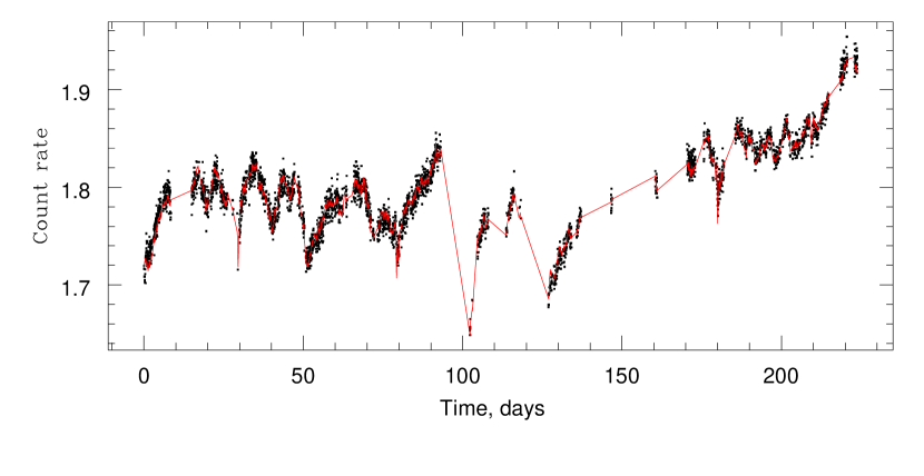
Figure 3: Count rate in the 900-1200 keV range (averaged over all 19 SPI detectors) as a function of time. Zero time corresponds to the beginning of the data set. The curve shows the predicted count rate in the same band based on a simple background model.

To verify the quality of the background model in the energy range of interest (i.e. around 511 keV) we used 0.5 Msec SPI observations of the Coma region. While these particular observations were also part of the data set used for the generation of the background model, they contribute only $\sim$10% to the total background exposure. Applying exactly the same procedure (described below) used for the Galactic Center observations we extracted the spectrum assuming that the spatial distribution of the line flux has a shape of a Gaussian with FWHM=6^∘centered at the Coma cluster (Fig.4 left panel). As for the Galactic Center observations we used an additional model consisting of a Gaussian plus constant (Fig.4 right panel). By construction the left plot is basically the difference between the spectrum coming from the Coma region and the mean spectrum over the entire background data set which contains many Galactic Plane pointings with bright sources. Therefore, a small negative bias, seen in the left panel of Fig.4, is a natural result. For the right panel (allowing for an additional free background component constant over all detectors) this negative bias is not present. For both panels no significant spectral features are present near the 511 keV line. For comparison we show in Fig.4 a line at 511 keV with parameters similar to those observed in the GC region. No evidence for spectral features near 511 keV is seen in the Coma field, suggesting that the background is removed with a sufficient accuracy.

Figure 4: Data points show the background subtracted spectra obtained from the 0.5 Msec SPI observations of the Coma region using the same procedure as is used for the Galactic Center region. For the left panel the spatial model is 6^∘Gaussian, centered at Coma cluster, while the background is fixed. For the left panel the model consists of a Gaussian plus a constant with the free normalization. For comparison superimposed on each plot is a Gaussian line at 511 keV (dotted lines; rebinned to the data resolution) with the total flux as seen from the GC region. An even $\sim$5 times weaker line would be seen in this 0.5 Msec observation.

2.4 Spectra extraction

For the GC spectra we use the data obtained when the main axis of the instrument was within 30^∘of the GC direction with an overall exposure time of $\sim$3.9 Msec (dead time corrected). The spatial model used is a simple Gaussian with FWHM ranging from 2 to 26^∘. Using available response files (results of Monte-Carlo modeling, described by Sturner et al., 2003) the count rate was predicted for every pointing and every SPI detector. Two models are used to extract the spectra. In the first model the normalization of the model (in a given energy band) was then obtained from a simple linear $\chi^{2}$ fit to the data:

$$\sum_{i}\left(\frac{A\times P_{i}-(D_{i}-B_{i})}{\sigma_{i}}\right)^{2}={\rm min},$$ (1)

where the summation is over the data set, $A$ is the normalization of the model (free parameter), $P_{i}$ is the model predicted rate, $D_{i}$ is the observed rate in a single detector during a given pointing, $B_{i}$ predicted background rate, and $\sigma_{i}$ is the standard deviation for the observed rate. In order to avoid bias due to the correlation of the observed rates $D_{i}$ and the errors $\sigma_{i}$ (see Churazov et al., 1996) we evaluate $\sigma_{i}$ using the exposure time of the $i-$th observation and the mean count rate (in a given detector and given energy band) averaged over a large number of observations. Since the absolute values of the variations of the count rate are small this procedure provides an unbiased estimate of $A$ with statistical uncertainty very close to the theoretical limit. The first model is essentially the difference between the flux measured from the GC region (weighted with a spatial Gaussian of a given width) and the mean spectrum over the data set used for the generation of the background model. For the second model we allow an additional background component (constant in time and space, but variable in energy) with a free normalization. I.e. in the second model the predicted count rate in the $i-$th observation is $A\times P_{i}+C$, where both $A$ and $C$ are free parameters. While the second model has an obvious advantage compared to the first model (see e.g. Fig.4), especially when trying to detect weak continuum radiation on top of the strong background line, the addition of the second free parameter increases (for the present data set) the statistical error in $A$ by a factor of 1.6 and 2.6 for the 2^∘and 26^∘Gaussian, respectively. We therefore extracted spectra using both models (hereafter model I and II) and checked the results for consistency.

The choice of these simple models (with the minimal number of free parameters) is primarily driven by a desire to get maximum significance in the resulting spectra. Observations during balloon flights (e.g. Harris et al., 1998) and with OSSE/CGRO (Kinzer et al., 2001) and earlier SPI imaging analysis (Knödlseder et al., 2003) indicate that a Gaussian is a reasonable first approximation for a 511 keV flux excess near GC even though the distribution might be more complicated than a simple Gaussian. In principle the assumed spatial distribution mainly affects the absolute normalization of the flux and to a lesser degree the spectral shape (unless the spectrum shape varies strongly across the studied area of the sky).

The total flux in the 508-514 keV band obtained using both models is shown in Fig.5 as a function of the Gaussian width. One can see that the flux changes from $\sim 0.5~{}10^{-3}{\rm ph~{}cm^{-2}~{}s^{-1}}$ to $\sim 2~{}10^{-3}{\rm ph~{}cm^{-2}~{}s^{-1}}$ as FWHM changes from 2 to 26^∘. The dotted line shows the behavior of $\chi^{2}$ in the model with a free constant (model II) as a function of the Gaussian width. Within this model the minimum $\chi^{2}$ is reached for the FWHM$\sim 6$^∘. The absolute value of the $\chi^{2}$ for 6^∘Gaussian is 0.9992 per degree of freedom (for 38969 d.o.f.). Given that the S/N for individual observation is very small, the absolute value of $\chi^{2}$ is not a very useful indicator of the acceptability of the model. However its closeness to unity shows that observed variations of count rates are very close to those expected from a pure statistical noise.

The width of the distribution suggested by the above analysis ($\sim$6^∘) is rather close to the value derived for the central bulge from OSSE observations (Kinzer et al., 2001), while the earlier analysis of a shorter SPI data set suggested a somewhat broader distribution $\sim$9^∘(Knödlseder et al., 2003) although consistent with 6^∘within the quoted uncertainties. The behavior of the curves in Fig.5 indicates that the 6^∘Gaussian does not account for the total flux of 511 keV photons coming from the GC region and an extra component (broader than 6^∘Gaussian) is needed. This result is robust against various assumptions on the SPI internal background. Since the topic of this paper is the shape of the annihilation spectrum we will not elaborate on particular spatial models. Subsequently we use only the spectra extracted using a 6^∘Gaussian. However, we verified that all the major spectral parameters (except for the overall normalization) are insensitive to the width of the spatial model.

Figure 5: Dependence of the flux in the 508-514 keV band on the width of the spatial Gaussian for model I with a fixed background (solid circles) and model II with a free constant background (solid squares). The dotted connecting solid triangles shows the behavior of the $\chi^{2}$ in model II.

Figure 6: Spectrum of the annihilation radiation from the GC region (6^∘Gaussian) in the 400-600 keV range derived from the model with the constant background as a free parameter (model II). For comparison a background spectrum, scaled by a factor of 0.01, is shown with a solid line. The annihilation line coming from the GC region thus corresponds to the level of $\sim$ 2-2.5% of the SPI background 511 keV. The observed continuum radiation below 511 keV is at the level of 0.4% from the instrument background continuum, except for the energies close to the positions of the strong background lines where the useful signal is at the level of 0.1% of the background.

3 Net spectra and spectral modeling

The spectra extracted with a 6^∘Gaussian, using two background models (fixed and free background), are shown in Fig.1 and Fig.6. The significance of the narrow line detection is 54.1 and 23.8 $\sigma$ respectively (based on the 508-514 energy band). When fitting the spectra over the energy range near 511 keV it was assumed that the SPI energy resolution is equivalent to the convolution of photon spectra with a Gaussian having FWHM $\sim$ 2.1 keV. For fitting spectral lines and the weak continuum on the red side of a line one has to verify the normalization and shape of the low energy tail in the SPI spectral response. At present a Monte-Carlo simulated SPI energy response matrix (spi_rmf_grp_0003.fits, Sturner et al., 2003) is available, which is constructed for broad continuum channels. According to this matrix the total off-diagonal tail of the SPI response for $\sim$511 keV photons amounts to $\sim$30% of the flux. The tail however is very extended (few hundred keV) and between 450 keV (lower energy boundary used for spectral fitting below) and 511 keV only about 3-4% of the line flux are due to off-diagonal response. Shown in Fig.7 is a typical situation one can expect for the GC spectra. The thin solid line shows a Gaussian line with a total intensity of unity. The dashed line is an ortho-positronium continuum with the total flux 4.5 times larger than the line flux (i.e. the case of annihilation through positronium formation). For comparison the dotted line shows the low energy tail of the narrow line estimated from the available response matrices. One can see that indeed the contribution of the tail is very minor (few per cent relative to the positronium continuum above 400 keV). We however routinely included this component in the subsequent spectral fitting, linking its flux to the normalization of the narrow 511 keV line. The impact of the off-diagonal tail on the continuum is even smaller and we neglected the tail in the continuum modeling. E.g. for the positroniuum continuum (the hardest continuum component used in the model) an account for the tail contribution above 450 keV can change the normalization by less than 2%. The flux ratio of the positronium continuum and the narrow 511 keV line determines the positronium fraction $F_{PS}=2/(1.5+2.25*F_{2\gamma}/F_{3\gamma})$, where $F_{2\gamma}$ and $F_{3\gamma}$ are the line and continuum flux, respectively. For large flux ratios (see Table 1) the positronium fraction is a weak function of the ratio and unless the Monte-Carlo simulated off-diagonal response is underestimated by a large factor (larger than $\sim$5) we do not expect any drastic changes in spectral parameters.

For the ortho-positronium continuum we use the spectrum of Ore & Powell (1949). To allow for broadening of the ortho-positronium continuum edge at 511 keV (SPI energy resolution and intrinsic broadening of the edge) we convolved the continuum with a Gaussian having a width from 2.1 to 7. keV. The fits were found to be fairly insensitive to the exact value of the edge broadening (unless it is very large) and instead of introducing an extra free parameter we fixed the width of the ortho-positronium edge at 4 keV.

The best fit parameters to the spectra are shown in Table 1. For comparison we show in Table 2 the spectral parameters derived by various missions in the past. It is clear that the results are in broad agreement. Deep INTEGRAL observations provide the most stringent constraints on the line centroid and on the width of the 511 keV line.

Figure 7: Estimated low energy tail (dotted line) of the bright line at 511 keV (solid line). The Monte-Carlo generated response matrix (Sturner et al., 2003) was used to estimate the tail. The total line flux is normalized to unity. For comparison an ortho-positronium continuum with the total flux 4.5 times larger than the line flux (i.e. the case of the annihilation through the positronium formation) is shown with the dashed line.

Table 1: Best fit parameters for the GC spectra calculated for a 6^∘(FWHM) Gaussian spatial model. Quoted errors are 1$\sigma$ for a single parameter of interest.

	Model I	Model II
	Fixed Background	Free Background
	485-530 keV	450-550 keV
	Single Gaussian + Ortho-positronium + power law
$E_{1}$, keV	510.988 [510.95-511.02]	510.954 [510.88-511.03]
$FWHM_{1}$, keV	2.47 [2.36-2.58]	2.37 [2.12-2.62]
$F_{2\gamma}~{}10^{-4}phot~{}s^{-1}~{}cm^{-2}$	$8.7\pm 0.20$	$7.16\pm 0.35$
$F_{3\gamma}~{}10^{-4}phot~{}s^{-1}~{}cm^{-2}$	$45.6\pm 4.3$	$26.1\pm 5.7$
$F_{3\gamma}/F_{2\gamma}$	5.2$\pm$0.51	3.65$\pm$0.82
$F_{PS}$	1.035$\pm$0.023	0.94$\pm$0.06
Power law photon index $\alpha$	2.0 (fixed)	2.0 (fixed)
$\chi^{2}$ (d.of.)	151.2 (83)	192.7 (193)

Table 2: Parameters of GC $e^{+}e^{-}$ annihilation spectrum obtained by various missions.

Instrument	Line energy (keV)	FWHMa (keV)	Positronium fraction	References
GRIS	–	2.5$\pm$0.4	–	Leventhal et al. 1993
HEAO-3	510.92 $\pm$ 0.23	1.6$\pm$1.35	–	Mahoney et al. 1994
HEXAGONE	511.53 $\pm$ 0.34	2.73$\pm$0.75	–	Durouchoux et al. 1993
OSSE	–	–	0.93$\pm$0.04	Kinzer et al. (2001)
TGRS	510.98 $\pm$ 0.1	1.81$\pm$0.54	0.94$\pm$0.04	Harris et al. (1998)
SPI/INTEGRAL	511.06 $\pm$ 0.18	2.95$\pm$0.5	–	Jean et al. (2003)
SPI/INTEGRAL	510.954 $\pm$ 0.075	2.37$\pm$0.25	0.94$\pm$0.06	this work

^a - the errors in FWHM were recalculated from the lower and upper limits on FWHM quoted in the original papers.

4 Constraints on the parameters of the annihilation medium

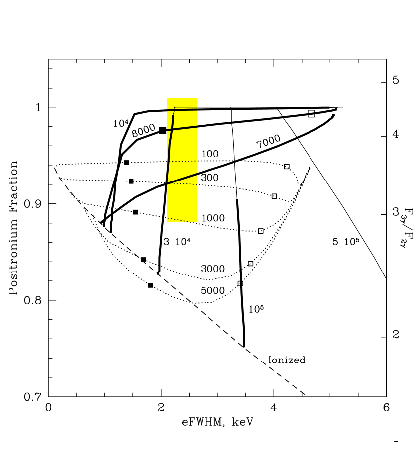
Figure 8: The effective FWHM of the 511 keV line versus the fraction of annihilation through the positronium formation. The gray area is the width and the positronium fraction observed by SPI. There are two groups of theoretical curves: cold - $T_{e}\leq 5000$ K (dotted lines) and warm/hot - $T_{e}\geq 7000$ K (solid lines). The temperature is fixed for each curve (the labels next to the curves), but the ionization fraction varies so that plasma changes from neutral to completely ionized along the curve. For cool temperature curves and for the 8000 K curve the points corresponding to the ionization degree of 0.01 and 0.1 are marked with the open and solid squares respectively. Each high temperature curve has two regimes, shown by thin and thick solid lines respectively. Thin (thick) lines correspond to the ionization fractions smaller (larger) than expected for collision dominated plasma at this temperature. For ISM the overionized state (regime shown by thick lines) is more natural than the underionized (thin lines). Finally the dashed line shows the relation between the line width and positronium fraction for a completely ionized plasma as a function of temperature.

Two observed quantities (the width of the line and the strength of the ortho-positronium continuum) impose some constrains on the temperature and ionization state of the annihilation medium. The positrons are assumed to be born hot, with the energy of order of few hundred keV and slow down by Coulomb losses (in ionized plasma) and ionization and excitation (in neutral gas). Once the energy of the positron drops below few hundred eV, charge exchange reactions with neutrals and/or radiative recombination or direct annihilation with free or bound electrons produce the annihilation line and the 3-photon continuum. The comprehensive description of the slowing down and annihilation of positrons in ISM is given by Bussard, Ramaty and Drachman (1979). Subsequent publications (e.g. Guessoum, Ramaty & Lingenfelter, 1991, Wallyn et al., 1994, Guessoum, Skibo & Ramaty 1997, Dermer & Murphy 2001) used updated values of the cross sections, but all principle results were in line with the conclusions of Bussard et al., 1979. For our calculations we considered pure hydrogen, dust free gas. For ionization, excitation and charge exchange reactions we used the theoretical cross sections of Kernoghan et al. (1996), which are in very good agreement with experimental data, for radiative recombination and direct annihilation with free electrons the approximations of Gould (1989), and for direct annihilation with bound electrons the results of Bhatia, Drachman & Temkin (1977). For positrons slowing down due to the ionization of hydrogen atoms, it is necessary to specify the distribution of scattered positrons over energy. For that purpose we use the distribution over the final energies predicted by the first Born approximation, while the normalization (total ionization cross section as a function of the positron initial energy) was kept at the Kernoghan et al. (1996) values. One can further correct the distribution over positron energy losses during ionization taking into account the enhancement of the cross section when final positron energy is approximately equal to the energy of the ejected electron (e.g. Mandal, Roy & Sil, 1986, Berakdar, 1998). This will be done in subsequent publications. For positrons slowing down due to interaction with free electrons we adopt the analytical approximation of Swartz, Nisbet & Green (1971) (see also Emslie 1978) derived for electron energy losses. For simplicity we used the cold target approximation, i.e. assumed that the positron energy is much higher than the temperature of the electrons. In our calculations we assume that charge exchange and radiative recombination form ortho- and para-positronium according to their statistical weights, i.e. 3 to 1, and we ignore the tiny contribution of the direct annihilation to the 3$\gamma$ continuum.

We use the Monte-Carlo approach to trace the history of positrons deceleration and the formation of the annihilation spectrum taking into account all the processes mentioned above. The spectrum produced by annihilation of thermalized positrons was calculated separately assuming a Maxwellian distribution of positrons over energy. Our estimates show that the deviations from the Maxwellian distribution, resulting from the charge exchange of positrons with neutral atoms, might affect the results of calculations only for a plasma with a temperature of $\sim$ 6000 K and a very low ionization fraction (less than $10^{-3}$), but not for any other combination of temperature and ionization state.

The predicted annihilation line does not have the shape of a true Gaussian and often contains a narrow component. The traditional definition of FWHM would then pick the narrow component and may miss the broader component. More informative would be the width of an energy interval which contains a given fraction of the line photons. To simplify the comparison with the results of previous missions and theoretical calculations we define the effective full width at half the maximum (eFWHM, Guessoum et al., 1991) of the line as an energy interval containing 76% of the line photons. For a true Gaussian eFWHM is equal to FWHM.

The results of the calculations are given in Fig.8, where each curve in Fig.8 corresponds to a particular value of temperature. The ionization fraction varies along each curve so that the ISM changes from neutral to completely ionized. One can identify two groups of curves in Fig.8 demonstrating different behavior.

The first group of curves corresponds to cool gas with a temperature below $\sim 6000$K. In the cold and neutral ISM about 94% of the positrons form positronium in flight, while the rest fall below the positronium formation threshold of 6.8 eV and eventually annihilate with bound electrons. The eFWHM of the line produced by positronium formation is $\sim$5.3 keV, while the annihilation with bound electrons produces FWHM of $\sim$1.7 keV (e.g. Iwata, Greaves & Surko, 1997) due to the momentum distribution of bound electrons. The eFWHM in the total annihilation spectrum is $\sim$4.6 keV. If the ionization fraction in the cold gas increases above $\sim 10^{-3}$, then Coulomb losses start to be important and the fraction of positrons forming positronium in flight decreases. For the positrons falling below 6.8 keV three processes are important - radiative recombination, annihilation with free electrons and annihilation with bound electrons. For ionization fractions of the order of a few $10^{-2}$ and temperatures $\sim 10^{3}$ K the annihilation with bound electrons causes the decrease of the net positronium fraction to $\sim$ 90-80%. If the ionization degree is more than a few per cent then only radiative recombination and annihilation with free electrons are important and the positronium fraction and the line width converge to the values expected for completely ionized plasma.

The second group of curves corresponds to temperatures higher than $\sim$7000 K. At these temperatures thermalized positrons can form positronium via charge exchange with hydrogen atoms and this process dominates over radiative combination and direct annihilation unless the plasma is strongly ionized. As a result for moderate degree of ionization the positronium fraction is very close to unity. Only when the plasma is significantly ionized (of the order of 6-10% for $\sim$8000 K gas and more for higher temperatures) the annihilation with free electrons starts to be important and the positronium fraction declines with increasing ionization degree (almost vertical tracks in Fig.8).

The above calculations probe the various combinations of the temperature and ionization, ignoring the physical possibility of such combinations. We now compare the results of INTEGRAL observations with the simulations and discuss plausible conditions.

The observed positronium fraction and the line width are shown in Fig.8 as a shaded rectangle. Comparing the simulated curves with the results of observations one can conclude that low and high temperature solutions are possible. The low temperature solution corresponds to temperatures below 1000 K, while for the high temperature solution falls into the range from 7000 to $4~{}10^{4}$ K.

4.1 Positrons annihilating in various ISM phases

The standard model of ISM in the Milky Way (e.g. McKee & Ostriker 1977, Heiles 2000, Wolfire et al., 2003) assumes that there are several distinct phases: Hot ($T_{e}\geq$ few $10^{5}$ K), Warm ($T_{e}\sim 8000$ K) and Cold ($T_{e}\leq 100$ K).

From Fig.8 it is clear that hot ($T_{e}\geq 10^{5}$ K) ionized medium does not give a dominant contribution to the observed annihilation spectrum. Indeed positrons annihilating in such a medium would produce too small positronium fraction and a much too broad annihilation line. One can increase the positronium fraction in such gas by requiring the low ionization fraction (i.e. increase the role of charge exchange) below the values expected in the collisionally ionized plasma. Such situation seems to be very unplausible and the width of the line remains too large anyway. One can easily limit the contribution of a very hot ($T_{e}\geq 10^{6}$ K), completely ionized plasma to the observed spectra, by adding a broad line to the fit. E.g. for $T_{e}=10^{6}$K the expected FWHM is $\sim$11 keV (Crannell et al., 1976) and the 90% confidence limit on the contribution of such a line to the observed flux is $\leq$ 17%. Given that at $10^{6}$K the direct annihilation and radiative recombination rates are nearly equal and assuming that the bulk of the remaining line photons are due to annihilation through the positronium formation, one can conclude that not more than $\sim$8% of positrons annihilate in a hot ($>10^{6}$ K) medium.

A qualitatively similar conclusion is valid for a cold ($T_{e}\leq$ $10^{3}$ K) neutral gas. While the positronium fraction is consistent with the observed one, the width of the line ($\sim$ 4.5 keV) is much too broad. One can decrease the line width by forcing a large ionization fraction (more than $10^{-2}$). For cold and dense gas (e.g. in molecular clouds or cold HI clouds) such an ionization fraction is much larger than expected.

On the other hand in the warm phase of the ISM ($T_{e}\sim 8000-10^{4}$ K) the ionization fraction varies substantially from less than $\sim$0.1 to more than 0.8. This phase alone can explain the observed annihilation line width and the positronium fraction. E.g. for 8000-$10^{4}$ K plasma one needs an ionization degree of several per cent to get both the line width and positronium fraction consistent with observations. For $2~{}10^{4}$ K plasma the ionization fraction has to be of the order of 0.4. At temperatures higher than $3~{}10^{4}$ K even plasma in collisional ionization equilibrium is strongly ionized ($>$99%). In real ISM one can usually expect stronger ionization than for collisionally ionized plasma. The corresponding parts of the curves in Fig.8 (i.e. ionization fraction larger than for collisionally ionized plasma) are shown by the thick solid lines.

Given the characteristic shapes of the curves in Fig.8 a combination of annihilation spectra coming from warm ISM and having various degrees of ionization could produce the annihilation spectrum consistent with observations. This conclusion is broadly consistent with earlier analysis of e.g. Bussard et al., 1979 or Guessoum et al. 1991.

4.2 The fraction of positronium formed in flight

Figure 9: The structure of the annihilation spectrum for 8000 K plasma with the degree of ionization $\sim$ 0.1. Dotted line shows the ortho-positronium continuum, short-dashed line is the 2-$\gamma$ decay of positronium formed in flight, thin solid line - 2-$\gamma$ decay of positronium formed by thermalized positrons, thin long-dashed line - direct annihilation of thermalized positrons. The thick solid line shows the total annihilation spectrum.

As was mentioned above, the shape of the annihilation line produced in the neutral or partly ionized medium can differ from a Gaussian. In fact for the majority of the theoretical curves in Fig.8 the annihilation line is composed of a rather broad FWHM $\geq$ 5 keV component (in flight positronium formation) and much narrower FWHM $\sim$ 1.0-1.7 keV component (due to radiative recombination with free electrons, charge exchange of thermalized positrons and annihilation with bound electrons). An example of the annihilation spectrum structure is shown in Fig.9. The broad component (dashed line) is due to in-flight positronium formation, while narrower components are associated with thermalized positrons. The same model spectrum (further smoothed with the SPI intrinsic resolution) is again shown in Fig.10 in comparison with the SPI spectrum. In terms of the $\chi^{2}$ such model yields comparable values, e.g. $\chi^{2}=192.2$ for 195 d.o.f. for the model with free background (cf. Table 1).

The change of the line width along the curves is primarily caused by the variation of the relative weights of these two components. Measurements of these weights would provide a more powerful test for the ISM composition than the effective width of the composite line. We therefore fit the observed spectra with the model consisting of two Gaussians instead of one as a simplified way to evaluate the contributions of in-flight and thermalized annihilations. Since for the in-flight positronium formation the width of the annihilation line depends only weakly on other parameters, we fixed the width of the second Gaussian at 5.5 keV, while the width of the first Gaussian remained free. The energy of the two Gaussians were set to be equal. Compared to the single Gaussian model (see Tables 1, 3) this model reduces the $\chi^{2}$ by 8.9 and by 3.9 for the “fixed background” and “free background” spectra respectively. Given that only one free parameter (normalization of the second Gaussian) is added to the model, the F-test suggests that the probability of getting such a reduction in $\chi^{2}$ is 2.6% and 5% for the two spectra, respectively.

Figure 10: The observed spectrum in comparison with a simple model of an annihilation spectrum of a warm 8000 K medium (ionization fraction 0.1) and a power law.

Table 3: Best fit parameters for the same spectra as in Table 1, when a second Gaussian with the width fixed at 5.5 keV is added. This second Gaussian mimics the broad line produced by the in flight positronium formation. Only essential parameters are quoted.

	Model I	Model II
	Fixed Background	Free Background
	485-530 keV	450-550 keV
	Double Gaussian + Ortho-positronium + power law
$FWHM_{1}$, keV	1.85 [1.64-2.03]	1.50 [1.25-1.89]
$F_{2\gamma}~{}10^{-4}phot~{}s^{-1}~{}cm^{-2}$	$6.63\pm 0.32$	$5.1\pm 0.69$
$FWHM_{2}$, keV	5.5 (fixed)	5.5 (fixed)
$F_{2\gamma}~{}10^{-4}phot~{}s^{-1}~{}cm^{-2}$	$2.50\pm 0.67$	$2.4\pm 0.96$
$\chi^{2}$ (d.of.)	142.35 (82)	189.0 (192)

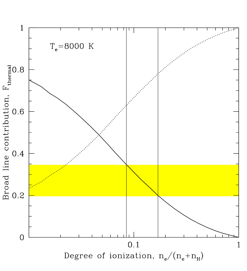
Figure 11: Contribution of the positronium, formed in flight, to the annihilation line (thick solid line) as a function of the ionization degree for 8000 K plasma. At this temperature thermalized positrons produce narrow line, while in flight positronium formation results in a broad component. INTEGRAL data (2 Gaussians fits) suggest that the contribution of the broad component is of the order of 30% (shaded region). Comparison with theoretical calculations shows that the most favorable degree of ionization is $\sim$0.1. The dotted line shows the fraction of thermalized positrons. For 8000 K plasma thermalized positrons produces a much narrower line than is produced in flight.

Using 2-Gaussian models one can conclude that the best fit fraction of the broad Gaussian in the total line flux is $\sim$30%. One can compare this value with the expected contributions of the broad (in flight) and narrow (thermalized) components in the warm medium as a function of the ionization degree as shown in Fig.11. One can see that for 8000 K plasma one needs ionization degrees in the range of 0.07-0.17 to have an appropriate relation between the broad and narrow components. As is mentioned above the curves shown in Fig.11 essentially reflect the changes of the positrons thermalized fraction as a function of the ionization state.

The same 2-Gaussian models can be used to get more quantitative constraints on the contribution of the cold neutral phase to the annihilation budget. The 90% confidence limit on the contribution of the broad (5.5 keV wide) Gaussian is $\sim$ 39%. Let us assume that this component is due to in-flight positronium formation in a cold neutral gas. About 6% of positrons in the cold gas fall below the positronium formation threshold and annihilate with bound electrons, thus contributing to the narrower component of the line. The conservative assumption that the rest of the positrons are thermalized in a warm ($\sim 10^{4}$ K) strongly ionized ($\geq$50%) medium and annihilate through the positronium formation implies an upper limit on the fraction of annihilations in the cold phase of 45%. Thus an approximately 1:1 mixture of cold neutral and warm ionized phases would produce a spectrum resembling the one observed with INTEGRAL. If instead a mixture of cold neutral and warm weakly ionized phases is considered, then the limits on the cold component contribution are stronger. If, for instance, the ionization degree of the warm phase is less than 10% then the cold component could not provide more than 10% of the annihilations. For warm phase with an ionization degree of 15% the limit on the cold component is $\sim$30%. Given the uncertainties in the determination of the mass fractions of various ISM phases (e.g. Heiles, 2000) the “natural” mixture of annihilations in proportion to the phase masses could also be consistent with the data.

A more detailed analysis of the INTEGRAL data (with an accurate separation of phases contributions and stringent constraints on the line components) will become possible once more data are accumulated and the knowledge of the instrument background and calibration is improved. More deep observations of the GC region are already planned and it should be possible to achieve at least a factor of 2-4 longer exposure of the GC during the next few years.

4.3 Width of the annihilation lines due to gas motions

For completeness we estimate the limits imposed by observations on the motions of the medium where positrons are annihilating.

First of all - a small statistical error on the line centroid achieved by SPI ($\sim$0.075 keV) corresponds to the uncertainty in velocity of $\sim$ 44 km/s. The measured line energy coincides (within the uncertainties) with the unshifted line and therefore there is no evidence of bulk motion of the annihilating medium with velocities larger than $\sim$40 km/s. Note that further improvement in the line statistics will require an accurate account for the Earth and Solar system motion relative to the GC since the magnitude of the velocities is of the same order.

The limits on the gas differential motions are not as strict. Consider e.g. the envelope of a star or supernova isotropically expanding with the velocity $v$. The intrinsically monochromatic line will then be observed as a boxy spectral feature with the full width of $1022\times\frac{v}{c}$ keV. One can then estimate the effective full width as $eFWHM\sim 2.6\left(\frac{v}{10^{3}~{}{\rm km/s}}\right)$ keV. Given that the observed width is $\sim$2.4 keV and for some ISM phases the intrinsic line can be relatively narrow $\sim$1-1.5 keV, velocities larger than $\sim 800~{}{\rm km~{}s^{-1}}$ can be excluded.

5 Conclusions

Deep observations of the Galactic Center region by SPI/INTEGRAL have yielded the most precise parameters of the annihilation line to date. The energy of the line is consistent with the laboratory energy with an uncertainty of 0.075 keV. The width of the annihilation line is constrained to $\sim$2.37$\pm$0.25 keV (FWHM) and the positronium fraction to 94$\pm$6%. Under a single phase annihilation medium assumption the most appropriate conditions are: the temperature in the range 7000-40000 K and the degree of ionization ranging from a few $10^{-2}$ for low temperatures to almost complete ionization for high temperatures. E.g. annihilation of positrons in one of the canonical ISM phases - 8000 K gas with an ionization fraction of $\sim$10% - would produce an annihilation spectrum very similar to the one observed by INTEGRAL. Under the assumption of annihilation in a multi-phase medium, the contribution of a very hot phase ($T_{e}\geq 10^{6}$ K) is constrained to be less than $\sim$8%. Neither moderately hot ($T_{e}\geq 10^{5}$ K) ionized medium nor very cold ($T_{e}\leq 10^{3}$ K) neutral medium can make a dominant contribution to the observed annihilation spectrum.

Further accumulation of the Galactic Center exposure with INTEGRAL and improvements in the background knowledge and calibration should make possible detailed fits of the data with the composite annihilation spectrum. Accurate separation of various components will place tight constraints on the width and the relative amplitude of annihilation features formed in flight and after thermalization. It will therefore be possible to make an accurate census of the distribution of annihilating positrons over ISM phases.

Simultaneously accurate information on the spatial distribution of the annihilation flux (especially in the latitudal direction) can be efficiently combined with the data on the spatial distribution of various ISM phases thus constraining the distribution of positron sources and the transport of positrons in the Galaxy.

6 Acknowledgements

We would like to thank SPI PIs V. Schoenfelder, G. Vedrenne, J.-P. Roques and V.L. Ginzburg, V.V. Zheleznyakov, A.M. Cherepashchuk, S.A. Grebenev and C. Winkler for their support. We are grateful to J.Berakdar, A.Lutovinov and L.Vainshtein for useful discussions and the referee, B. J. Teegarden, for a very helpful report.

This work is based on observations with INTEGRAL, an ESA project with instruments and science data center funded by ESA member states (especially the PI countries: Denmark, France, Germany, Italy, Switzerland, Spain), Czech Republic and Poland, and with the participation of Russia and the USA.

The dominant part of the GC exposure used in the paper comes from deep (2 Ms) GC observations carried out as part of the Russian Academy of Sciences share of the INTEGRAL data.

References

- [\citeauthoryearBerakdar1998] Berakdar J., 1998, PhRvL, 81, 1393
- [\citeauthoryearBhatia, Drachman, & Temkin1977] Bhatia A. K., Drachman R. J., Temkin A., 1977, PhRvA, 16, 1719
- [\citeauthoryearBrown & Leventhal1987] Brown B. L., Leventhal M., 1987, ApJ, 319, 637
- [\citeauthoryearBussard, Ramaty, & Drachman1979] Bussard R. W., Ramaty R., Drachman R. J., 1979, ApJ, 228, 928
- [\citeauthoryearChurazov et al.1996] Churazov E., Gilfanov M., Forman W., Jones C., 1996, ApJ, 471, 673
- [\citeauthoryearCourvoisier et al.2003] Courvoisier T. J.-L., et al., 2003, A&A, 411, L53
- [\citeauthoryearDermer & Murphy2001] Dermer C. D., Murphy R. J., 2001, In: Exploring the gamma-ray universe. Proceedings of the Fourth INTEGRAL Workshop, 4-8 September 2000, Alicante, Spain. Editor: B. Battrick, Scientific editors: A. Gimenez, V. Reglero & C. Winkler. ESA SP-459, Noordwijk: ESA Publications Division, ISBN 92-9092-677-5, 115
- [\citeauthoryearDurouchoux et al.1993] Durouchoux P., et al., 1993, A&AS, 97, 185
- [\citeauthoryearEmslie1978] Emslie A. G., 1978, ApJ, 224, 241
- [\citeauthoryearGuessoum, Ramaty, & Lingenfelter1991] Guessoum N., Ramaty R., Lingenfelter R. E., 1991, ApJ, 378, 170
- [\citeauthoryearGuessoum, Skibo, & Ramaty1997] Guessoum N., Skibo J. G., Ramaty R., 1997, The Transparent Universe, Proceedings of the 2nd INTEGRAL Workshop held 16-20 September 1996, St. Malo, France. Edited by C. Winkler, T. J.-L. Courvoisier, and Ph. Durouchoux, European Space Agency, 113
- [\citeauthoryearGould1989] Gould R. J., 1989, ApJ, 344, 232
- [\citeauthoryearHarris et al.1998] Harris M. J., Teegarden B. J., Cline T. L., Gehrels N., Palmer D. M., Ramaty R., Seifert H., 1998, ApJ, 501, L55
- [\citeauthoryearHeiles2001] Heiles C., 2001, Tetons 4: Galactic Structure, Stars and the Interstellar Medium, ASP Conference Series, Vol. 231. Edited by Charles E. Woodward, Michael D. Bicay, and J. Michael Shull. San Francisco: Astronomical Society of the Pacific, 294
- [\citeauthoryearIwata, Greaves, & Surko1997] Iwata K., Greaves R. G., Surko C. M., 1997, PhRvA, 55, 3586
- [\citeauthoryearJean et al.2003] Jean P., et al., 2003, A&A, 407, L55
- [\citeauthoryearJohnson, Harnden, & Haymes1972] Johnson W. N., Harnden F. R., Haymes R. C., 1972, ApJ, 172, L1
- [\citeauthoryearJohnson & Haymes1973] Johnson W. N., Haymes R. C., 1973, ApJ, 184, 103
- [\citeauthoryearKernoghan et al.1996] Kernoghan A. A., Robinson D. J. R., McAlinden M. T., Walters H. R. J., 1996, JPhB, 29, 2089
- [\citeauthoryearKinzer et al.2001] Kinzer R. L., Milne P. A., Kurfess J. D., Strickman M. S., Johnson W. N., Purcell W. R., 2001, ApJ, 559, 282
- [\citeauthoryearKnödlseder et al.2003] Knödlseder J., et al., 2003, A&A, 411, L457
- [\citeauthoryearLeventhal, MacCallum, & Stang1978] Leventhal M., MacCallum C. J., Stang P. D., 1978, ApJ, 225, L11
- [\citeauthoryearLeventhal et al.1993] Leventhal M., Barthelmy S. D., Gehrels N., Teegarden B. J., Tueller J., Bartlett L. M., 1993, ApJ, 405, L25
- [\citeauthoryearMahoney, Ling, & Wheaton1994] Mahoney W. A., Ling J. C., Wheaton W. A., 1994, ApJS, 92, 387
- [\citeauthoryearMandal, Roy, & Sil1986] Mandal P., Roy K., Sil N. C., 1986, PhRvA, 33, 756
- [\citeauthoryearMcKee & Ostriker1977] McKee C. F., Ostriker J. P., 1977, ApJ, 218, 148
- [\citeauthoryearOre & Powell1949] Ore A., Powell J. L., 1949, PhRv, 75, 1696
- [\citeauthoryearSturner et al.2003] Sturner S. J., et al., 2003, A&A, 411, L81
- [\citeauthoryearSwartz al.1971] Swartz, W. E., J. S. Nisbet, and A. E. S. Green, 1971, J. Geophys. Res., 76, 8425
- [\citeauthoryearTeegarden et al.2004] Teegarden B. J., et al., 2004, ApJ accepted, astro-ph/0410354
- [\citeauthoryearVedrenne et al.2003] Vedrenne G., et al., 2003, A&A, 411, L63
- [\citeauthoryearWallyn et al.1994] Wallyn P., Durouchoux P., Chapuis C., Leventhal M., 1994, ApJ, 422, 610
- [\citeauthoryearWeidenspointner et al.2003] Weidenspointner G., et al., 2003, A&A, 411, L113
- [\citeauthoryearWinkler et al.2003] Winkler C., et al., 2003, A&A, 411, L1
- [\citeauthoryearWolfire et al.2003] Wolfire M. G., McKee C. F., Hollenbach D., Tielens A. G. G. M., 2003, ApJ, 587, 278