Structure Function Analysis of Long-Term Quasar Variability

Abstract

In our second paper on long-term quasar variability, we employ a much larger database of quasars than in de Vries, Becker & White. This expanded sample, containing 35 165 quasars from the Sloan Digital Sky Survey Data Release 2, and 6 413 additional quasars in the same area of the sky taken from the 2dF QSO Redshift Survey, allows us to significantly improve on our earlier conclusions. As before, all the historic quasar photometry has been calibrated onto the SDSS scale by using large numbers of calibration stars around each quasar position. We find the following: (1) the outbursts have an asymmetric light-curve profile, with a fast-rise, slow-decline shape; this argues against a scenario in which micro-lensing events along the line-of-sight to the quasars are dominating the long-term variations in quasars; (2) there is no turnover in the Structure Function of the quasars up to time-scales of $\sim$40 years, and the increase in variability with increasing time-lags is monotonic and constant; and consequently, (3) there is not a single preferred characteristic outburst time-scale for the quasars, but most likely a continuum of outburst time-scales, (4) the magnitude of the quasar variability is a function of wavelength: variability increases toward the blue part of the spectrum, (5) high-luminosity quasars vary less than low-luminosity quasars, consistent with a scenario in which variations have limited absolute magnitude. Based on this, we conclude that quasar variability is intrinsic to the Active Galactic Nucleus, is caused by chromatic outbursts / flares with a limited luminosity range and varying time-scales, and which have an overall asymmetric light-curve shape. Currently the model that has the most promise of fitting the observations is based on accretion disk instabilities.

1 Introduction

The cause of the long-term variability in quasars is still a matter of debate. Unlike the short time-scale variations (on the order of days), which are adequately described in terms of relativistic beaming effects (e.g., Bregman et al., 1990; Fan & Lin, 2000; Vagnetti et al., 2003), the variations at much longer time-scales (years to decades) are less understood. Current scenarios under consideration are ranging from source intrinsic variations due to Active Galactic Nucleus (AGN) accretion disk instabilities (e.g., Shakura & Sunyaev, 1976; Rees, 1984; Siemiginowska & Elvis, 1997; Kawaguchi et al., 1998; Starling et al., 2004), and possible bursts of supernovae events close to the nucleus (e.g., Terlevich et al., 1992; Cid Fernandes et al., 1996), to source extrinsic variations due to micro-lensing events along the line-of-sight to the quasar (e.g., Hawkins, 1993, 2002; Alexander, 1995; Yonehara et al., 1999; Zackrisson et al., 2003). See also the review article by Ulrich, Maraschi & Urry (1997).

Determining which of the various proposed mechanisms actually dominates quasar variability is best done by studying it toward the longest possible time-baselines. Depending on the mechanism, each has markedly different variability “power” at the longer time-scales (e.g., Hawkins, 2002). This means that if one would have a quasar monitoring sample that is both large enough, and covers a large enough time-baseline, one could address these issues adequately. Unfortunately, given the nature of monitoring programs, this is not something that can be started overnight. The longest quasar light-curve monitoring programs are on the order of 20 years (e.g., Hawkins, 1996), and will take a long time before they are expanded significantly in time-baseline.

The way around this is by using historic photographic plate material, in combination with a recent survey. Like in our previous paper (de Vries, Becker & White, 2003, hereafter Paper I), we chose to use the Sloan Digital Sky Survey (SDSS), Data Release 2 (DR2), in combination with the historic Second Generation Guide Star Catalog (GSC2, McLean et al., 1998) and the Palomar Optical Sky Survey (POSS, Reid et al., 1991). This allows for photometric information on the quasars spanning up to 50 years. The downside is that, unlike the monitoring programs, we have typically a very sparse light-curve sampling per quasar. However, since we will have a very large number of them, the sampling across the complete database will be very good. This obviously only works if the variability of the quasars is due to a mechanism common to all quasars. We proved the validity of this concept in Paper I, and recently a similar approach has been taken by Sesar et al. (2004).

The paper is outlined as follows: In § 2, we introduce the quasar sample, and we will argue that it can be considered a representative sample of the overall quasar distribution. Section 2.2 goes through the careful calibration steps needed before one can properly start interpreting the results. The method outlined is in principle the same as in Paper I, but since the sample is much larger, it does allow for some enhanced corrections. In § 3, we will introduce the variability diagnostic used throughout the paper: the Structure Function (hereafter SF). This measure has been used extensively in the literature, and allows for easy and direct comparison with long-term variability studies based on the monitoring of individual quasars (e.g., Hawkins, 2002). In addition, Kawaguchi et al. (1998) modeled SF behavior depending on the intrinsic variability mechanism. Clear differences in the SF curves are expected depending on whether the dominant variability is due to either bursts of supernovae close to the nucleus, instabilities in the accretion disk, or intervening micro-lensing events. Throughout the paper we will refer back to the predictions made in Kawaguchi et al. (1998).

Section 3.2 describes the results of the calibration on the stellar SF. The purpose of this detailed section is twofold: first, it reflects the level of data-quality we have attained with the calibration method, and secondly, it identifies subtle effects on the data that may have gone unnoticed by just focusing on the quasar SF. Among other things, the clear differences in photometric data-quality between the POSS and GSC2 surveys only shows up significantly in the stellar SF. Also, the Malmquist bias signal is clearly seen in the stellar SF, whereas it is masked (and indeed washed out) in the quasar SF by the light-curve asymmetry signal (cf. § 3.3.6).

Section 3.3 and its subsections detail the results we obtained for our quasar sample. These are discussed in light of the existing literature data and our last section on SF modeling in § 4.

2 Sample Selection and Calibration

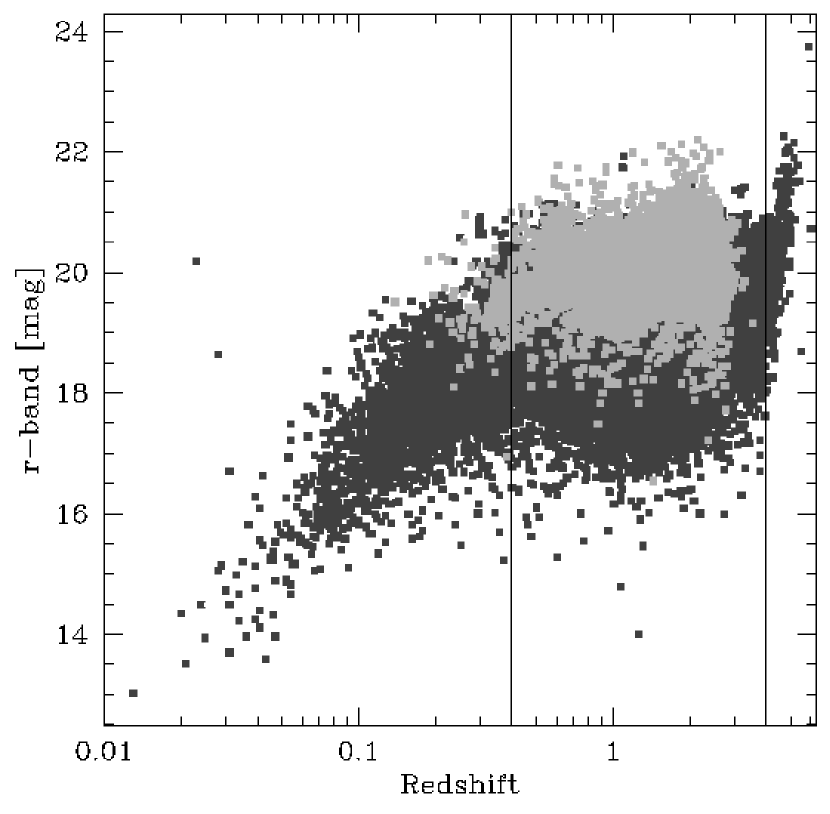
Figure 1: Distribution of quasar $r_{\mbox{\tiny SDSS}}$-band magnitudes as function of redshift. The dark squares are quasars from the DR2 data-set, and the light squares are (spectroscopically confirmed) 2dF quasars that have photometric DR2 data. The two vertical lines demarcate the redshift range of 0.4 to 4 for which the $r_{\mbox{\tiny SDSS}}$-band distribution is more or less independent of redshift. Outside these boundaries a strong correlation between redshift and magnitude exists.

In order to significantly improve on our work in Paper I (using 3791 quasars from the SDSS Early Data Release), we had to wait until the later releases would increase the quasar sample by a large amount. This was accomplished by the two subsequent Data Releases, which expanded the database first to 16 908, and then to 35 165 quasars (Data Release 2). This DR2 is described in detail in Abazajian et al. (2004). In addition, we added all the 2dF quasars (Croom et al., 2004) that are covered by the DR2, but are not among the 35 165 in their quasar database. This increases the sample size to 41 578 quasars, all of which have accurate and recent SDSS photometric information. However, since we are interested in historic variability, we had to remove the 187 quasars that were not included in either the POSS or the GSC2 catalogs. This leaves us with the final sample of 41 391 quasars. Table 1 has the exact break-down of photometric information on this sample.

Table 1: Quasar Sample

Quasars	Photometric Epochs
32,832	SDSS GSC POSS I
8,530	SDSS GSC
29	SDSS GSC POSS I
41,391

2.1 Photometric Properties

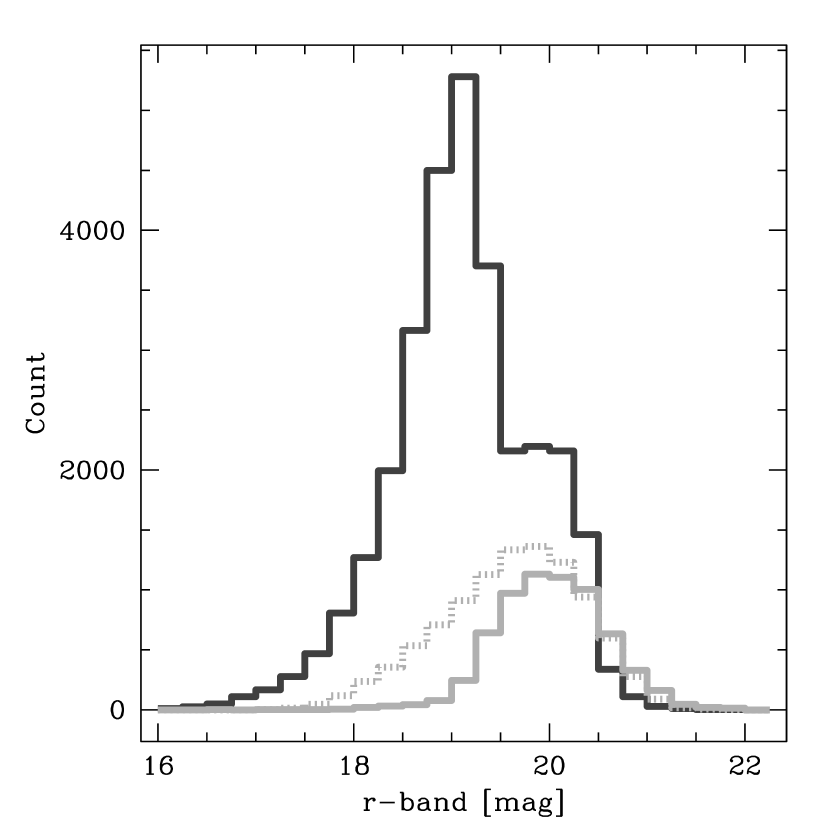
Figure 2: Histograms of the magnitude distribution for quasars with redshifts between 0.4 and 4. The dark-colored histogram is for the DR2 data only, and the light-colored lines are for the additional 2dF quasars. The dashed histogram shows all the 2dF quasars in the DR2 area, and the solid gray histogram just the ones that are not in the DR2 sample. It is clear that different selection criteria were used for the SDSS and 2dF surveys. The SDSS appears to have a bimodal magnitude distribution, whereas the 2dF is more uniformly distributed around $r_{\mbox{\tiny SDSS}}$=19.8.

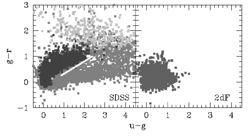
Figure 3: Plot of the DR2 and 2dF quasars (left and right panel) in the $(u-g)$ and $(g-r)$ color plane. This is one of the planes used to select quasar candidates for spectroscopic follow-up with SDSS (e.g., Richards et al. 2002). The stellar locus is indicated by the thick solid white line, and illustrates the intrinsic color differences between stars and quasars (hence the relative paucity of quasars in that area). The SDSS sample has been divided into three redshift bins (colored from dark to light): $z<0.4$, $0.4<z<4$, and $z>4$. Note the limited color range of the 2dF quasars compared to the SDSS selection criteria.

Figure 1 shows the $r_{\mbox{\tiny SDSS}}$-band magnitude of the sample as function of redshift. The faintest quasars are about $r_{\mbox{\tiny SDSS}}$=21, except the very highest redshift quasars ($z>4$), which clearly have been selected using different criteria. The lower redshift sources ($z<0.4$) also show a correlation between their redshift and optical magnitude. At these redshifts the quasar host galaxy is contributing significantly to the overall luminosity, and progressively more so with decreasing redshift. This non-variable host galaxy component will lower the relative variability amplitude of the AGN. If, for instance, the AGN varies intrinsically by 10%, placing it inside a galaxy with the same magnitude will lower the variability of the combined system to 5%. The optical variability of an individual quasar is not just a function of AGN luminosity relative to its host galaxy luminosity, it also depends on the redshift of the source. First, the contrast between the AGN and its host galaxy increases dramatically toward the restframe blue and UV wavelengths (as probed by the passbands even at moderate redshifts). Second, the $(1+z)^{4}$ cosmological surface brightness dimming factor affects the extended galaxy more than the point-source AGN contribution, again increasing the contrast between the two components. Both these redshift dependent trends diminish the unwanted variability-lowering effect by the host galaxy, and based on Fig 1, it does not appear to contribute beyond $z\approx 0.4$.

The bulk of our quasars (36  802) have redshifts between 0.4 and 4.0 (marked in Fig. 1), whereas 4424 (or about 10% of the sample) are at redshifts below 0.4 and might potentially be affected by their host galaxies. A direct comparison between the results with and without the low redshift data-set did not yield any significant differences, except at the longest time-lags in the $r_{\mbox{\tiny SDSS}}$-band in particular (see § 3.3.5).

The quasars added from the 2dF survey have a different brightness distribution (cf. Fig. 1, light-colored points) than the SDSS quasars, mainly because of different selection criteria. This difference remains, even if we put the 2dF and DR2 overlap quasars back into the 2dF sample, as is clearly illustrated in Fig. 2. Both the SDSS and 2dF use multi-band photometric criteria to preselect for quasar candidates. In addition, the SDSS sample has been augmented by targeting FIRST and ROSAT counterparts as well (Richards et al., 2002), and in general uses a less restrictive color cut. The fraction of radio- and X-ray loud sources is relatively low (2692 FIRST counterparts within 2″, and 479 ROSAT counterparts within 15″), so it does not significantly alter the distribution.

Figure 3 illustrates the differences between the SDSS and 2dF selected quasars. The sources have been plotted on the $(u-g)$ and $(g-r)$ plane, which is one of the color-color diagrams used in selecting SDSS quasar candidates (Richards et al., 2002). The 2dF quasar candidates were selected from scanned UK Schmidt Telescope (UKST) photographic plates, with magnitudes ranging from $18.25<b_{\mbox{J}}<20.85$. In addition, the candidates had to satisfy one of the following criteria (see Croom et al., 2004): $u-b_{\mbox{J}}\leq-0.36$; $u-b_{\mbox{J}}<0.12-0.8(b_{\mbox{J}}-r)$; or $b_{\mbox{J}}-r<0.05$. This results in a markedly different color and ($r$-band) magnitude distribution from the SDSS quasars. However, the important similarity is that the redshift distribution between $0.4<z<4$ is fairly uniform as function of $r$-band magnitude (cf. Figs. 1 and 2). So, even though the quasars have been selected differently, and actually populate the color-color diagram of Fig. 3 differently, we feel that there is no a-priori bias in either sample with respect to variability in general, and variability on select time-scales in particular.

2.2 Photometric Calibration

Calibration of historic photographic plate material can be achieved by virtue of using large numbers of random field stars around the (quasar) position of interest. Plate-to-plate variations in emulsion quality, and even variations within a single plate can contribute significantly to measurement uncertainties. So, even though the POSS I and GSC2 catalogs have been calibrated carefully (as a whole), and brought up to CCD photometric standards, there is still a lot of improvement to be made by recalibrating the photometry. We basically follow the same procedure as outlined in Paper I by using all the available photometry for the field stars within 5′ of the quasar position. This typically amounts to (depending on the epoch) anywhere between 50 to 500 stars. We like to stress that this “local” calibration is to be preferred over complete plate corrections due to the potential inhomogeneities inherent to photographic plates (e.g., Lattanzi & Bucciarelli, 1991; Gal et al., 2003).

We will go over the calibration process step by step, but we will refer to the calibration sections in Paper I where appropriate. Most of the next discussion will highlight the improvements we were able to make on the old procedure, mainly due to the much larger data-set.

The first step is to calculate the best passband transformations for each quasar individually, using the nearby field stars. The transformations involved are, for the POSS I: $B$ to $g_{\mbox{\tiny SDSS}}$, and $R$ to $r_{\mbox{\tiny SDSS}}$. Note that the $B$ and $R$ magnitudes are already transformed to the Johnson passbands from their photographic $O$ and $E$ emulsions (see Reid et al. 1991, and Monet et al. 2003 for the $B$ and $R$ transformations). For the GSC2 plates, the relevant color transformations are $J$ to $g_{\mbox{\tiny SDSS}}$, and $F$ to $r_{\mbox{\tiny SDSS}}$. In principle, our transformation will take care of the proper passband corrections, possible plate / weather variations, and the fact that SDSS uses AB magnitudes whereas the catalogs are on the Vega system. However, an important caveat we like to emphasize here is that the “best transformation” is defined as the particular transformation that results in the smallest color rms for the stars. As we have explained in Paper I, this does not necessarily translate into the best calibration for the quasars, which after all, is the transformation we are interested in. There are two main contributors to this stellar-quasar disparity: their optical spectrum is completely different (cf. Fig. 3 of Paper I), and quasars typically have powerful emission lines which depending on their redshift, may, or may not, be present in the passband. These emission lines can account for upward of a few tenths of a magnitude of the total brightness. Both these differences between the field stars and the quasars render the stellar transformation less than ideal. It is something we can correct for, however.

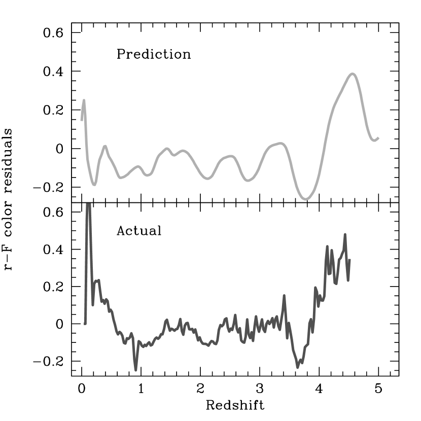
Figure 4: Residual $r_{\mbox{\tiny SDSS}}$$-F$ color differences after applying the best stellar transformation to the quasar magnitudes, as function of redshift. The lower panel shows the actual median of the distribution ($\sim 40\,000$ quasars). The top panel depicts the expected color changes, based on a quasar template spectrum, and a mean stellar spectrum of a K2V star (cf. Paper I). Note the excellent agreement between the two curves, except for the lowest redshift range (which is affected by the host galaxy contribution, cf. § 3.3.5).

Figure 4 illustrates this calibration best. The bottom panel shows the median $r_{\mbox{\tiny SDSS}}$$-F$ color for our quasar sample as function of redshift. Ideally, these residuals should be close to zero after calibration in the absence of emission lines and quasar-stellar spectral differences. This is clearly not the case. However, these color excursions (of up to more than 0.2 in magnitude) are closely matched by what one would expect using quasar and stellar template spectra (top panel). As explained in Paper I, we get the best agreement between the actual residuals and the theoretical ones by assuming a mean stellar template of a K2V star. This stellar type is consistent with expectations based on population models for our Galaxy (e.g., Bahcall & Soneira, 1980, 1981). So, the fact that these color excursions are well understood in terms of quasar emission lines moving in and out of the observing passband, makes it clear that we have to correct for it. If left “untreated” it will affect the variability SF directly by artificially inflating the rms values at certain time-lags. Given the epoch distribution of the observations (time-lags preferentially at $\sim 1$, $\sim 10$, and $\sim 50$ years), the redshift maps more or less directly onto a particular time-lag. The strong excursion at $z\approx 3.6$, for example, would skew the SF signal preferentially at $10/(1+3.6)\approx 2$, and $50/4.6\approx 11$ years. In this paper we opted to use the actual median, as calculated across bins with a width of 0.05 in redshift units, over the modeled offsets. This accounts much better for the low ($z<0.4$) redshift quasars which are increasingly more contaminated (with decreasing redshifts) by their host galaxies.

All of the other passband transformations are treated similarly. The result is that each historic passband has been brought onto their SDSS counterpart (either $g$ or $r$), with the important distinction that the color distributions are centered around $0$ as a function of redshift. This method improves significantly over the procedure outlined in Paper I. There, bulk corrections have been applied to the color distributions (irrespective of redshift). Figure 2 of Paper I can therefore be considered a projection of Fig. 4 onto the $y$-axis. Only with the large increase in sample size were we able to actually correct for the redshift dependence in a meaningful way.

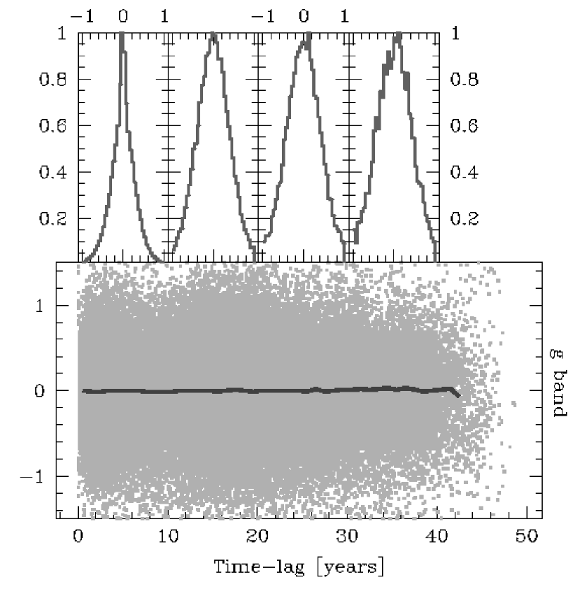
Figure 5: Quasar variability distribution in the $g_{\mbox{\tiny SDSS}}$-band as function of time-lag. This distribution has been calibrated as described in the text. The thick solid line indicates the local median value of the distribution, and its lack of significant deviation from zero serves as an indication of our careful calibration. The top 4 histograms are for the time-lag bins [0, 10$>$, [10, 20$>$, [20, 30$>$, and [30, 40$>$ years respectively. The increase of the FWHM with increasing time-lag is evident. The bin values are: 0.57, 0.94, 1.00, and 1.05 magnitude. Note that the first histogram deviates by quite a bit from a Gaussian distribution. The other three are accurately described by one.

After all the photometric data have been transformed onto the SDSS passbands, the measurements for each individual quasar are permutated among each other, resulting in about 4 time-lag measurements per band per quasar. Obviously, none of the individual quasars have been sampled photometrically anywhere near enough to produce a meaningful structure function for each quasar individually. The combined data-set, however, allows for detailed variability studies provided one assumes that the underlying cause of quasar variability is the same for all of them. We will get back to this issue in § 4.

This final data-set (one each for the $g_{\mbox{\tiny SDSS}}$- and $r_{\mbox{\tiny SDSS}}$-bands) contains sorted pairs of time-lag (in years) and magnitude difference. For our sample of 41 391 quasars, this amounts to 170 102 individual measurements for the $g_{\mbox{\tiny SDSS}}$-band, and 131 123 for the $r_{\mbox{\tiny SDSS}}$-band. This exceeds the total number of permutations in Paper I by more than an order of magnitude. The difference in the totals between the bands is because some GSC2 photometry for the quasars have been repeated more in the $J$ than in the $F$ band, boosting the permutation numbers for the $g_{\mbox{\tiny SDSS}}$-band.

The actual data for the $g_{\mbox{\tiny SDSS}}$-band have been plotted in Fig. 5. The bottom panel shows the magnitude differences as function of intrinsic time-lag. Since the quasars are quite spread out in redshift space (cf. Fig.1), we have to bring the actual time separation between the observations onto the reference frame of the quasar itself (by dividing it by a $(1+z)$ factor). This has the additional advantage of smoothing out the time-lag distribution. So even though the observing campaigns were well separated in time (1950’s, 1990’s, and $\sim 2000$), resulting in time-lags clustering around a few, $\sim 10$, and $\sim 50$ years, the $(1+z)$ redistributing factor results in a pretty smooth distribution up to time-lags of $\sim 40$ years (cf. Fig. 5, bottom panel).

The top four panels of Fig. 5 provide a direct picture of the increase in FWHM (and hence the rms) of the magnitude difference distribution as time-lags increase. This is actually the definition of the SF (see next section). Since the total number of time-lag measurements decreases with increasing time-lag, this is not immediately obvious looking at the point-cloud in the lower panel. The numbers of data-points for the current 10-year time-lag binning are: 86 795, 50 974, 22 627, and 8 520 permutations respectively. While the numbers do decline, they are still large enough to assess the FWHM of the distribution very accurately. The last bin alone already contains 30% of the total number of permutations used for Paper I.

3 Structure Function

Our analysis of Paper I, and the current paper, will utilize the SF as the tool to characterize the quasar variability. SF’s are not very sensitive to aliasing problems due to discrete and/or sparse time sampling (e.g., Hughes et al., 1992), which make them well suited for our purpose. As before, we define the SF as:

$$S(\tau)=\left(\frac{1}{N(\tau)}\sum_{i<j}{[m(i)-m(j)]^{2}}\right)^{\frac{1}{2}}$$ (1)

with the summation over all the combinations of measurements for which $\tau=t_{j}-t_{i}$. In our case we group all the $n(n-1)/2$ permutations into bins which contain at least 200 measurements. The SF value for each bin is then given by the rms of the magnitude permutations.

3.1 Error estimates

This results in $\sim$1500 bins, which are then binned again onto a fixed grid in log time-lag space (running from $-0.97$ to 1.55 in 0.06 dex bins for a total of 42). This facilitates easy comparison between model and actual SF curves. It also allows us to approximate the error on a particular SF point by calculating the rms of the $1500/42\approx 36$ values inside each bin. This is basically the same method as we employed in Paper I. The presented error-bars reflect therefore accurately the actual local SF uncertainties. It should be stressed that, unlike a well monitored SF of a single source for which all of the bins are cross-correlated with each other and an objective error estimate is hard to give, our bins are essentially independent. Out of the 150 000 or so time-lag measurements (per band) only measurements for a single quasar (about 4) are correlated with each other. In other words, each of the SF bins contains a virtually completely different set of quasars. This bin-independence also allows us to quantify SF similarities in terms of their offset distributions. Assuming two SF curves, labeled $A$ and $B$, both of which are binned to the same $N=42$ bins specified above, we can define:

$$\overline{O}=\frac{1}{N}\sum_{i}^{N}{S_{A}(i)-S_{B}(i)}$$ (2)

$$\Delta\overline{O}=\frac{\sigma}{\sqrt{N}}=\frac{1}{N}\left(\sum_{i}^{N}{\left(S_{A}(i)-S_{B}(i)-\overline{O}\right)^{2}}\right)^{\frac{1}{2}}$$ (3)

after substituting $N\approx\sqrt{N}\sqrt{N-1}$. The quantities $\overline{O}$ and $\Delta\overline{O}$ represent the mean SF offset and its $1\sigma$ uncertainty, respectively. We will use this metric in particular for our SF asymmetry part of the paper.

3.2 Stellar Structure Function

The SF for the calibration stars serves multiple purposes. If we assume that stars, on average, are not variable, then the SF derived from it should not exhibit any correlation with time-lag. In other words, it should be parallel to the $x$-axis (in plots like Fig. 6). This was indeed found to be the case for the stars in Paper I, which clearly illustrated the significant differences between the SF behavior of stars and quasars. However, given the much smaller sample sizes for Paper I (note that the number of calibration stars is linked to the number of quasars), the overall stellar SF was rather noisy. It just served to make the point that constructing an SF from a random sample of stars resulted in a non-variable SF curve, but it clearly was not good enough to go beyond that. The current sample, however, is large enough. In the next few sections, we will discuss the stellar SF in more detail.

3.2.1 Stellar Type Dependencies

In the same way spectral differences between the average stellar spectrum and a quasar spectrum lead to slightly different passband corrections, and therefore, additional noise to the variability measure, spectral differences among stars themselves will inflate its SF variability signal as well. This has to be considered in the construction of the stellar SF. The reason we can use stars to calibrate the quasars at all, is that the mean of the stellar color distribution does not change that much going from one sightline to another. The stellar population therefore does not change a lot across the sky covered by DR2.

In order to limit the stellar spectral range allowed for our template SF, we only included stars within a magnitude range ($17<r<21$), and an $(r-g)$ color within 0.2 magnitudes of the typical stellar color of $(r-g)=0.4$ (cf. Stoughton et al., 2002). This color cut effectively limits the allowed range of stellar colors, and improves the passband calibrations accordingly. The resulting time-lag permutation database contains 2.1 million data-points (over both bands), an order of magnitude larger than the quasar permutation database. The net effect is a lowering of the SF, especially for the GSC data (below time-lags of 10 years). The POSS I data, plotted separately in Fig. 6, retains a slightly higher noise plateau, mainly due to the photometric data quality differences between the GSC and POSS surveys.

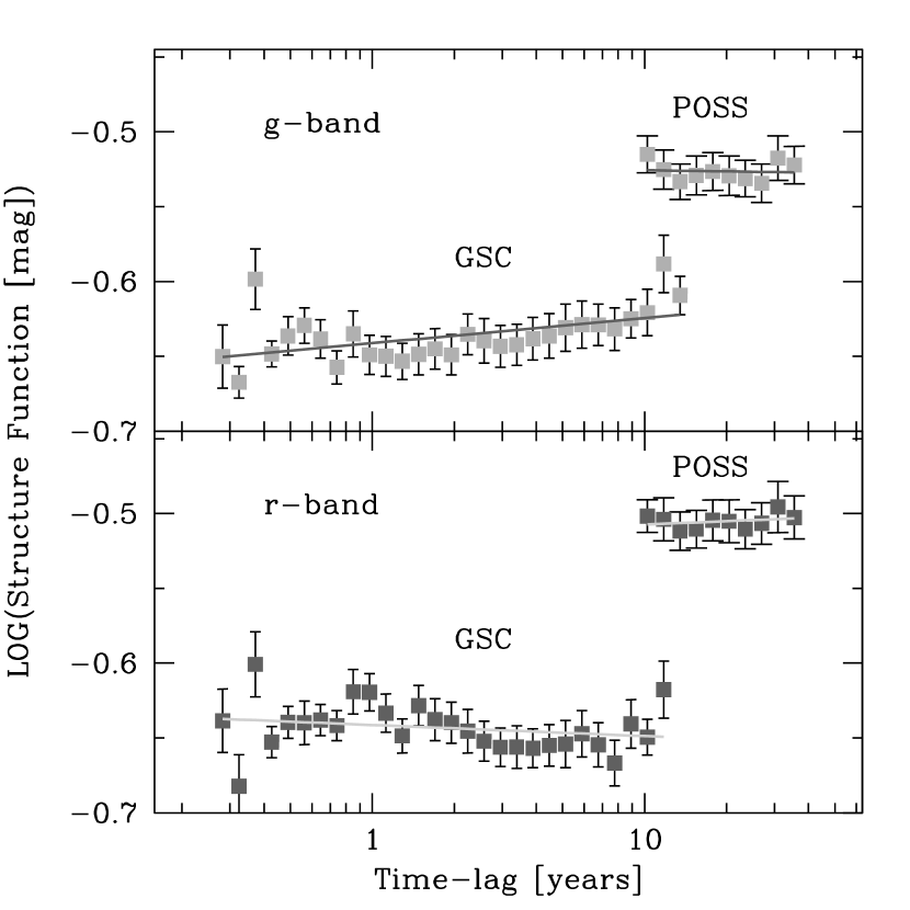
Figure 6: Structure functions of calibration stars; SDSS $g$-band in the top panel, and SDSS $r$-band in the bottom panel. The data quality of the earlier POSS survey is lower than that of the GSC, resulting in a slightly higher noise plateau. The solid lines are least squares fits to the data points. The slopes are: $+0.017\pm 0.006$ (GSC-$g$), $-0.003\pm 0.012$ (POSS-$g$), $-0.008\pm 0.006$ (GSC-$r$), and $+0.007\pm 0.009$ (POSS-$r$).

Because of this data quality difference, we have separated out the GSC and POSS contributions to the stellar SF in Fig. 6. Linear least squares fits to the data-points have been made, and their slopes are: $+0.017\pm 0.006$ (GSC-$g$), $-0.003\pm 0.012$ (POSS-$g$), $-0.008\pm 0.006$ (GSC-$r$), and $+0.007\pm 0.009$ (POSS-$r$). With the possible exception of the $g$-band SF for the GSC data, none of the slopes differ significantly from zero (i.e., no correlation with time-lag). Even the GSC-$g$ case is only weakly increasing with time-lag with the highest SF value within $1\sigma$ of the lowest. It should also be noted in this respect that the small SF excursions from the mean in the GSC-$r$ case are not statistically significant.

The main result from this exercise is twofold. First, there is no significant correlation between the SF for stars and the time-lag for both the GSC and POSS data. This implies that any signal we detect in the quasars beyond the stellar SF curve must be due to the quasars themselves. Also, it is not clear how much of the stellar SF signal is due to intrinsic color scatter, and how much can be attributed to measurement noise. Recently, Sesar et al. (2004) estimated the photometric error in the GSC2 and POSS I to be 0.10 and 0.15 magnitude, respectively. They used individual SDSS plates (100 square arcminutes) to correct the POSS I and GSC2 photometric catalogs. Taken at face value, these uncertainties translate into a white noise signal in the SF at levels of $-0.85$ and $-0.67$, using Eqn. 3 from Paper I. Both these levels are lower than the plateaus we measure in our stellar SF. How much of this difference can be attributed to the different calibration method, and how much can still be improved upon by even more carefully designed color-cuts, is unknown. As a consequence, we cannot “correct” the quasar SF by subtracting a measurement-noise component, and instead, like in Paper I, we will have to include a white noise term in our Monte Carlo models.

Figure 6 presents the final corrected SF for both the $g_{\mbox{\tiny SDSS}}$- and $r_{\mbox{\tiny SDSS}}$-bands. As measured from the figure, the final SF levels, separated into time-lags less and more than 10 years, are: $-0.63$ and $-0.53$ for $g_{\mbox{\tiny SDSS}}$, and $-0.64$ and $-0.51$ for $r_{\mbox{\tiny SDSS}}$. The corresponding formal noise levels are: 0.17, 0.21 and 0.16, 0.22 magnitudes. The POSS I levels are only slightly lower than found in Paper I, but the GSC2 levels are suppressed by about 0.10 (in SF units).

3.2.2 Malmquist Bias in the Structure Function

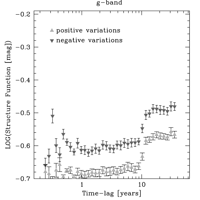
Figure 7: The $g$-band Structure Functions for the calibration stars (using the narrow $(r-g)$ color set), separated in positive-only (light-gray symbols) and negative-only (dark-gray symbols) variations. Positive variations are defined as brightening with increasing time (i.e., the SDSS epoch is the brightest), and negative variations have the opposite sign (i.e., the SDSS brightness is less than what it was at the older epochs). The offset between the two SF curves is due to the Malmquist bias, acting upon the subset of the calibration stars that are variable. Note that, unlike in Fig. 6, the GCS and POSS data have been combined, resulting in a slightly smoother transition across time-lags of 10 years.

Leading up to the construction of the SF is an intermediate step in which we take care to center the distribution of variations around $0$, as function of time-lag (see Fig. 5 for the quasar case), without changing the shape of the distribution. If there is any asymmetry present in the distribution, we can test for it by looking at the positive and negative sides of the distribution separately. The variations are defined with respect to the newest epoch, so positive variations imply that the source is brighter (i.e., had a lower magnitude) than it was before, and negative variations imply that the source is fading with time. This definition is consistent with the one used in Kawaguchi et al. (1998).

For a perfectly symmetric variation distribution, the positive and negative SF curves should be identical. This, however, is clearly not the case for our calibration stars. Figure 7 shows the SF for the positive (light-gray triangles) and negative variations (dark-gray triangles) separately. Since the SF curves are not identical, it indicates an asymmetric variation distribution. In the next few paragraphs we will argue that this asymmetry is due to the Malmquist bias in our stellar sample. It basically means that for the subset of our stars that have intrinsic variability, the ones that were a lot fainter at the earlier epochs (i.e., the positive variations) would not make it into either the POSS I or GSC2 catalogs (given their brightness limits), thereby reducing the rms / SF signal. Variations in the other direction are not affected by this since there is no upper brightness limit to the catalogs. The net effect is a skewing in the variation distribution.

There are some important points to be made based on the SF curves in Fig. 7. First, both SF curves are the same, except for a constant offset in log (which translates into a $\sim 14\%$ increase in rms). This implies two things: 1) The Malmquist bias does not depend on time-lag (and it should not), nor does it depend on the quality of the photometry. The POSS I measurements are noisier than the GSC2 ones, but there is no evidence for a different offset between the positive and negative SF curves. 2) The magnitude of the stellar variability is not correlated to intrinsic time-lag because we are not sensitive to their time-scales, quite unlike the variations for the quasars (see § 3.3).

The second observation we like to make is that, on top of the uncertainty about the exact contribution of measurement noise to the SF (cf. § 3.2.1), this asymmetry induced SF signal further compounds the problem of disentangling the SF into its various contributions. Therefore, we cannot use the stellar SF to improve or correct the quasar SF.

3.2.3 Variable star contribution

Sesar et al. (2004) quote a variable star fraction (with variability exceeding 0.2 magnitude) of at least 1% of the population. The rms difference between the positive and negative SF curves (from Fig. 7) is actually not that large: for the shorter timescales, we measure rms = 0.148 and rms = 0.177 mag for the positive and negative SF curves. Since this 0.029 magnitude difference is not that large, a small fraction of variable stars might be enough to skew the distribution. For sufficiently large distributions (where $(N-1)/N\approx 1$), the rms of two distributions, each with its own $\sigma$, can be combined as follows:

$$rms=\left(\frac{N_{1}}{N_{1}+N_{2}}\sigma_{1}+\frac{N_{2}}{N_{1}+N_{2}}\sigma_{2}\right)^{1/2}$$ (4)

with $N_{1}$, $N_{2}$ the total number of items in each distribution. In our case, we assume the following for the non-variable part of the stellar distribution: $\sigma_{1}=0.13$, and $N_{1}=99N_{2}$ (i.e., only 1% of the sample is variable). We also have to assume that this $\sigma_{1}$ scatter is symmetric around $0$, and is small enough not to be affected by the Malmquist bias. It is in effect a constant contribution to both of the SF curves. All of the Malmquist signal therefore has to be ascribed to the variable subset of stars.

We can make the observations agree with our simple distribution model by assuming that half of the variable stars vary with on average 0.5 magnitude, and the other half varies by 1.5 magnitude. Since we are looking out of the Galactic plane, and do not make any a-priori assumptions about the stars (other than that they are found close to a quasar), the main constituents of the variable star population are RR-Lyrae and Asymptotic Giant Branch (AGB) stars. Neither the magnitude of their variation, nor their relative fractions are inconsistent with the values we assume here (see, e.g., Derue et al., 2002).

It is the high variability part that drops out on the positive variation side of the distribution (i.e., the half with the 1.5 magnitude variability). This results in the following rms values: $\sigma_{\mbox{neg}}=1.12$ and $\sigma_{\mbox{pos}}=0.50$ magnitude. By applying Eqn. 4, we arrive at total rms values of 0.148 and 0.179, very close to the actual values. Obviously, none of these values are constrained to any degree, they just serve to demonstrate that we can actually explain the observed stellar SF curves by the Malmquist bias due to a small percentage of variable stars.

We will come back to the asymmetry issue in the next Section, where we discuss the SF of our quasar sample.

3.3 Quasar Structure Function

Figure 8: Combined $g_{\mbox{\tiny SDSS}}$- and $r_{\mbox{\tiny SDSS}}$-band structure function for the quasar sample (dark squares). The least-squares slope of the SF is: $(0.153\pm 0.004)$ with intercept $(-0.557\pm 0.003)$ at time-lags of 1 year. The SF curves for the $r_{\mbox{\tiny SDSS}}$- and $g_{\mbox{\tiny SDSS}}$-bands are indicated separately. Note that we limited the redshift range for the $r_{\mbox{\tiny SDSS}}$-band curve to $z>0.6$ (see § 3.3.5). The clear break in the stellar SF curve at low noise levels (cf. Fig. 6), due to the varying data quality, does not affect the SF curve for quasars.

Our quasar SF curve is presented in Fig. 8 by the dark-gray squares. It is immediately clear that this SF curve is a vast improvement over the one presented in Paper I (Fig. 7), with a much smaller scatter of the points. The individual error-bars are actually small enough to allow for detailed modeling, something that the data quality did not allow for in Paper I. Before we continue, however, we like to establish the reality of the quasar SF curve by comparing it to currently the best long-term one available in the literature.

3.3.1 Literature comparison

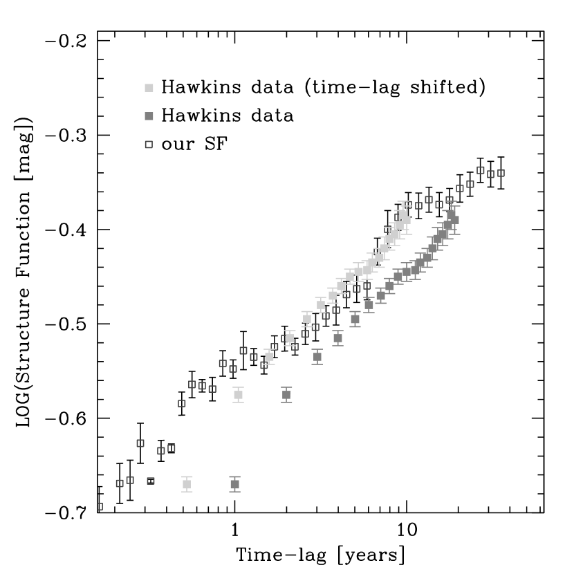
Figure 9: Comparison of our quasar SF with a literature SF based on long-term monitoring of 401 quasars (Hawkins 2002). The original Hawkins data have not been corrected for time-dilation (dark-gray squares), but can be made to agree with our SF by applying a 0.3 dex shift toward shorter time-lags (light-gray squares). This corresponds to a sample mean offset of $z=1$. Note that, except for the 2 shortest time-lag bins, all the Hawkins data points are within $1\sigma$ of our points. Our short time-scale measurements are most likely shifted upward a bit due to the intrinsically higher level of measurement noise (compared to the Hawkins data set).

This paper’s approach to long-term quasar variability is quite different from the monitoring approach, in which one repeatedly measures the brightnesses of a fixed sample of quasars. Given our statistical method, which uses archival photometry data and a less than straightforward calibration path, one might have concerns about the results. We therefore compare our resulting quasar SF to the highest quality available long-term quasar SF from the literature (taken from Hawkins 2002). This SF was constructed based on $\sim 30$ year monitoring data on a sample of 401 quasars, and is plotted with our SF in Fig. 9. The Hawkins SF, which has not been corrected for time-dilation, is represented by the dark-gray squares. Since our data have been corrected by the $(1+z)$ term, we have to shift the Hawkins SF over toward shorter time-scales. The light-gray squares have been shifted leftward by 0.3 dex (corresponding to a sample mean redshift of 1). This shifting does not affect the slope of the SF, as mentioned in, e.g., Kawaguchi et al. (1998); Hawkins (2002). Note that, with the exception of the shortest two time-lag data points, all of the Hawkins data can be made to fall within $1\sigma$ of our curve. The offset at short time-scales is most likely due to the higher photometric accuracy (and hence a correspondingly lower noise plateau) of the Hawkins data compared to our data (for which these data points will be shifted upward a bit, see Fig. 6 from Paper I).

It is reassuring to see that these two different approaches, each with their own set of clearly distinct potential systematic problems, produce SF curves that are so alike.

We do like to remind our reader that, even though the curves are similar, there is a key difference: our data bins are almost completely independent with different quasars contributing to different bins, whereas in the Hawkins SF, most bins contain data (permutations) from the same set of quasars. This is a big advantage when one tries to understand the SF errors (cf. § 3.1) and the potential differences between positive- and negative-variation SF curves (cf. § 3.3.6).

3.3.2 Lack of SF turnover

There are a few things we like to discuss based on our quasar SF in Fig. 8. First of all, there is no indication that the SF curve is turning over, consistent with the results from Hawkins (2002). What we are looking for in the SF curve is the presence of a consistent plateau beyond a certain time-scale (cf. Fig. 16, and Hughes et al. (1992)), and not necessarily an actual “peak” in the SF curve. A significant drop in the SF signal beyond a particular time-scale usually indicates problems with adequate time sampling at those time-lags. In our case, the SF curve might be affected beyond $\sim 40$ years due to the decrease in available time-lags (remember that the intrinsic time-scale are shortened by the $(1+z)$ time-dilation factor). We do not see such a drop, however, and the possible leveling off seen in the last few bins is not significant enough to claim we have detected a preferred variability time-scale.

This is not to say that there is no upper bound to the variability time-scale, just that we do not have any sensitivity to it.

3.3.3 Color dependencies

The second clear trend in our SF is that the $g_{\mbox{\tiny SDSS}}$ SF curve has more signal (i.e., is more variable at any given time-lag) than the $r_{\mbox{\tiny SDSS}}$ SF curve. This is consistent with quasars being intrinsically more variable at shorter wavelengths. This is not a new result (it was also present, albeit at rather low significance, in Paper I), but is now very clearly detected.

Giveon et al. (1999) measured a $0.02$ magnitude rms difference between B- and R-band variability in their sample of 42 Palomar Green (PG) quasars. Trevese & Vagnetti (2002) found variability shifts of these magnitudes between the blue and red to be consistent over a range of samples. Wavelength variations in the near-IR tend to be smaller, and are possibly too small to be measured (Enya et al., 2002a). Possible mechanisms for these spectral variations include nuclear star-bursts / supernovae which are predominantly blue (e.g., Aretxaga et al., 1997; Cid Fernandes et al., 2000), and instabilities in the nuclear accretion disk (e.g., Kawaguchi et al., 1998; Giveon et al., 1999; Trevese & Vagnetti, 2002).

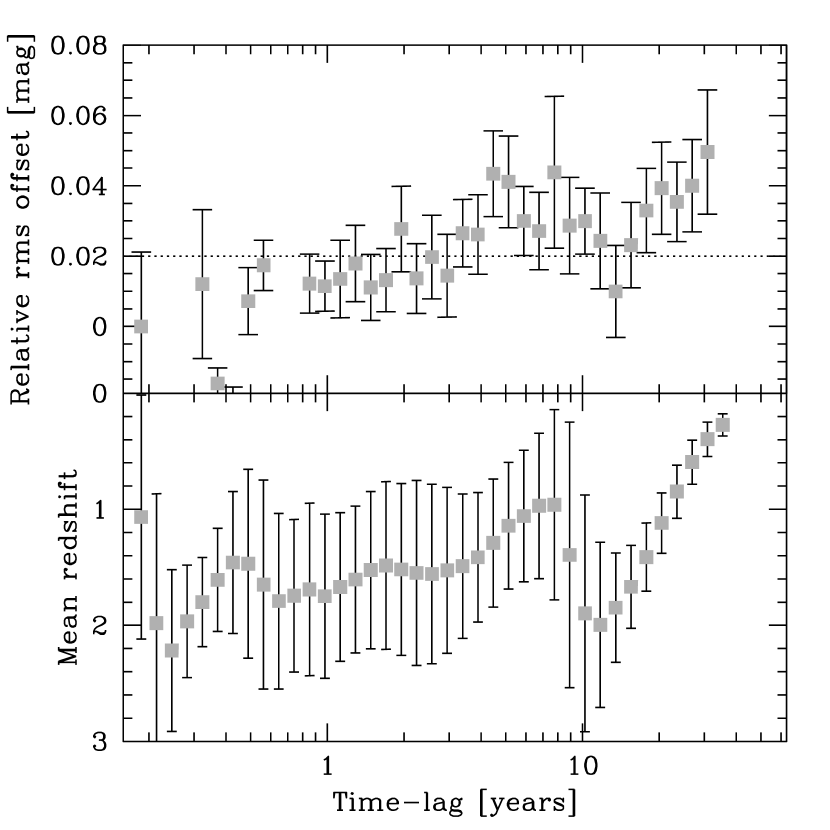
Figure 10: The top panel depicts the change in the offset between the $g_{\mbox{\tiny SDSS}}$- and $r_{\mbox{\tiny SDSS}}$-band variability as function of time-lag. This offset is not constant since the $r$- and $g$-band SF curves in Fig. 8 are diverging. The dashed line is the constant $0.02$ mag color offset as measured by Giveon et al. (1999). Our mean value offset value is $0.027$, for time-lags larger than 1 year (the shorter time-lag data are rather noisy). In the bottom panel, the mean redshift as a function of time-lag is plotted. The error-bars indicate the 1$\sigma$ spread in the $z$-distribution within the bin, and should not be taken as the error in the mean redshift value (which is given by $\sigma/\sqrt{N}$). The mean redshift and relative color offsets are correlated to better than 99.9% significance.

Figure 10 shows the SF color offset as a function of time-lag. In the top panel, we have plotted the observed rms offset between the $g_{\mbox{\tiny SDSS}}$- and $r_{\mbox{\tiny SDSS}}$-band SF curves, as function of time-lag in the quasar restframe. It appears that the increase in color offset correlates with time-lag, but it is actually the redshift that the color offset depends on. In the bottom panel we have plotted the mean redshift of the quasars contributing to a particular time-lag. Since the time-lags have been converted into the restframe of the associated quasar, a $(1+z)$ factor has shortened the epoch separation. This implies that the very longest time-lags ($>40$ years) can only include data from the lowest redshift quasars, a trend clearly seen in the plot. Now, assuming the quasar variability introduces a spectral slope change (i.e., it is bluer during an outburst, cf. Trevese & Vagnetti, 2002; Vagnetti et al., 2003) the biggest color contrast is attained when the observed passbands are furthest apart. This would be the case for redshift zero objects. At higher redshifts, one starts to probe progressively bluer parts of the spectrum, and the spectral separation between the $g_{\mbox{\tiny SDSS}}$- and $r_{\mbox{\tiny SDSS}}$-bands becomes smaller and smaller. This effect of decreasing color contrast with increasing sample mean redshift is accurately portrayed in Fig. 10. Even the sudden increase in mean redshift around the 10-year time-lag bins is reflected by the drop in the relative rms change. The Spearman rank coefficient for the correlation between the mean redshift and the color offset (beyond time-lags of 1 year) is $-0.73$. This translates for the 23 degrees of freedom into a less than 0.1% likelihood that the correlation is by chance.

This good correlation between the two suggests an intrinsic origin to the variability. However, this does not rule out the per definition extrinsic micro-lensing scenario. It is possible that by assuming a $(1+z)$ time-dilation correction in the first place, we have introduced some correlation between mean redshift and color offset. Given the fact that we rely on the $(1+z)$ term to smooth out our time-lag coverage, we cannot produce a similar plot without such a $(1+z)$ correction to test this. Nevertheless, a stronger argument against a lensing scenario is the presence of a light-curve asymmetry signal in the SF curve (cf. § 3.3.6).

3.3.4 SF slope

The predicted slopes for the starburst (SB) and accretion disk instability (DI) models are $(\alpha=0.83\pm 0.08)$ and $(\alpha=0.44\pm 0.03)$, respectively (Kawaguchi et al., 1998). Note that both these slopes are significantly steeper than our measured value of $(\alpha=0.153\pm 0.004)$, which is far closer to the modeled micro-lensing slopes ($\alpha\approx 0.25\pm 0.03$), and a bit shallower than the $0.20\pm 0.01$ slope of the Hawkins (2002) data.

It was this inconsistency between the measured quasar SF slope and the predicted SB and DI slopes that led Hawkins to propose a micro-lensing origin of long-term quasar variability. Our data, based on the slope of the SF alone, seems to support this contention. It also implies that, in the case micro-lensing is ruled out, that either or both of the other models need significant modification to explain the observed slope.

As we pointed out in Paper I (Fig. 6), the measurement noise does have a direct effect on the slope of the SF. The larger the noise, the shallower the slope. Since our data is noisier than the photometric observations used by Kawaguchi et al. (1998) for their modeling, we will come back to the slope issue in § 4.1.3 where we construct a noise-less SF.

3.3.5 Host galaxy contamination

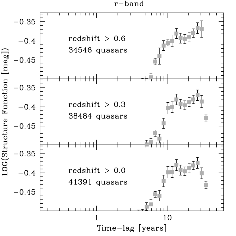
Figure 11: Effect of the quasar host galaxy on the AGN variability SF (for the $r_{\mbox{\tiny SDSS}}$-band in this case). The lowest redshift sources contribute the most to the longest time-lags. It is these bins that are most affected, due to a combination of cosmological surface brightness dimming and the progressively smaller (red) galaxy contribution at blue and UV restframe wavelengths. The three panels show that the “turn-over” at long time-lags disappears if one increases the low-redshift cut-off. Also none of the other bins are affected, a nice illustration of the lack of correlation between the bins. Note that we only detected this effect in the $r_{\mbox{\tiny SDSS}}$-band and not in the $g_{\mbox{\tiny SDSS}}$-band. This is consistent with the notion that the host galaxies are intrinsically red.

Variability in quasars is associated with their AGN. A large, non-varying, host galaxy might therefore limit the relative variation if one uses integrated magnitudes. Since we are not attempting any galaxy / AGN decomposition, and just use the total magnitude, this might be somewhat of a concern. The sharp upturn in residual $r-F$ colors toward low redshifts (cf. Fig. 4, or Fig. 1 of Paper I) already hinted that this might be at play at low redshifts. In this section we will quantify this effect on the SF curve. Figure 10, bottom panel, shows that the low-redshift sources dominate the longer time-lag bins, and that the largest effects are to be expected here. This is confirmed in Fig. 11, which plots the long time-lag part of the SF, with different low redshift thresholds. The apparent turnover at the extreme end of the bottom SF curve (which includes all data), disappears if one removes all the quasars below redshifts of 0.6. Evidently, the host galaxy contribution is enough to lower the variability signal at these redshifts. Clearly, if one wants to study variability of AGN using a nearby sample, this has to be taken into account. In our case, a simple removal of the nearby quasars is enough, since none of the other SF bins are affected (again thanks to our bin independence).

It should also be noted that this turnover is not present (or at least has not been detected) in the $g_{\mbox{\tiny SDSS}}$-band. This is consistent with the notion that the AGN is more dominant at shorter wavelengths, whereas a galaxy is usually much redder.

In further discussions about the $r_{\mbox{\tiny SDSS}}$-band SF curve, we have removed these quasars (10% of the total) from the sample. The $g_{\mbox{\tiny SDSS}}$-band data-set is unaffected.

3.3.6 Light-curve asymmetry

Asymmetries between the rising and falling parts of the light-curve can be investigated by separating the variations in positive and negative variations only (cf. § 3.2.2). Kawaguchi et al. (1998) model various scenarios of variability, each with different SF signatures. Their starburst (SB) model has a very short rise time, followed by a long exponential decay (cf. their Fig. 2). They also consider an accretion disk instability (DI) model for which the variations rise slowly, but fall off rapidly (basically in a saw-tooth like pattern, cf. their Fig. 5). The SF curves derived from these light curves both have significant asymmetries between the positive and negative variations. They are, predictably, of opposite nature: the fast-rise, slow-decline of the SB model results in more SF signal in the positive variations, whereas the slow-rise, fast-decline DI model has more signal in the negative variations. This behavior can be intuitively understood in terms of the SF having typically more variability signal at the fast changing part of the light curve compared to the slowly changing part, for a given time-lag. In a sense the SF mirrors the derivative of the light curve.

Figure 12 shows this asymmetry for our data. We only show data for the $g_{\mbox{\tiny SDSS}}$-band because the SF offset between the $g_{\mbox{\tiny SDSS}}$- and $r_{\mbox{\tiny SDSS}}$-bands is of the same order of magnitude as the asymmetry signal (cf. Fig. 8), so combining both bands is not helpful. The positive variations (light-gray symbols) have more SF signal than the corresponding negative ones (they are binned the same way in time-lag). This is a strong indication that the typical quasar variations are not symmetric, and behave in a fast-rise, slow-decline way. This is consistent with the modeled light curves we used in Paper I (see Fig. 5) and the SB-like light curves, but appears at odds with the inferred behavior of the DI models. Furthermore, the asymmetry effect we see in the calibration stars (cf. § 3.2.2), and which we interpret as a sign of Malmquist bias, works in the opposite sense. This increases the significance of the disparity between the positive and negative variations for our quasar sample. Indeed, based on modeled SF curves for which we force the light-curves to be time-symmetric, we consistently measure a mean offset between the positive and negative variations of $\overline{O}=0.000\pm 0.003$ (based on Eqns. 2 and 3). For our actual quasar sample these values are $\overline{O}=0.027\pm 0.003$, which makes it significant at the 6.4$\sigma$ level.

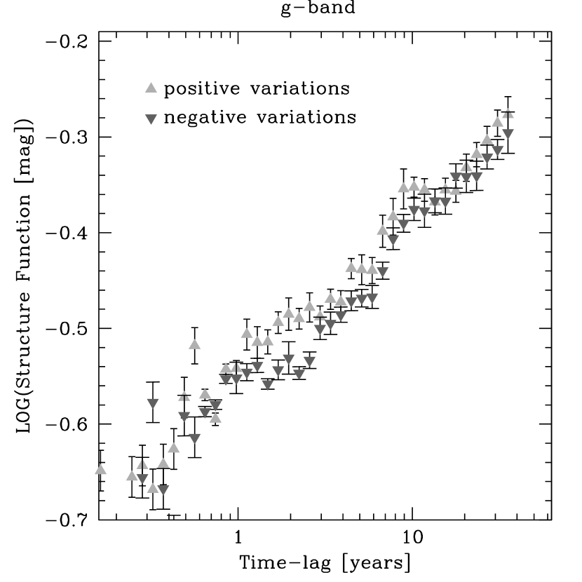
Figure 12: The $g$-band Structure Functions for the quasars, separated into positive-only (light-gray symbols) and negative-only (dark-gray symbols) variations (see Fig. 7 for their definitions). Since the positive SF curve has more signal than the negative one (which is the exact opposite of the stellar case), it is a clear indication of asymmetric variability (i.e., the rise and decline parts of the light-curve are not identical). The mean offset along the $y$-axis is $\overline{O}=0.027\pm 0.003$ (for time-lags beyond 1 year), which is equivalent to a 0.020 magnitude offset in rms.

Another trend that does not appear in our data is for the two SF curves to merge beyond the typical time-scale of the variation. Both the SB and DI models of Kawaguchi et al. (1998) display this behavior, whereas our SF curves remain offset and parallel as function of time-lag. This is an indication that there does not appear to be a preferred time-scale in our quasar sample. In § 4.1.2, we will actually argue for a continuum of variation time-scales.

3.3.7 Asymmetry implications for the micro-lensing scenario

If variations are asymmetric in time, and either spend the least time rising or declining in brightness, offsets will appear in the SF between the positive and negative variations (e.g., Kawaguchi et al. 1998, and § 4.1.2), given enough of an asymmetry. This asymmetry signal persists under arbitrary time-dilation corrections: a $(1+z)$ correction merely compresses the time-scales, it does not alter the intrinsic shape of the light-curve. Neither does it change the slope of the SF (e.g., Kawaguchi et al., 1998; Hawkins, 2002). The same statements are true for symmetric variations: there is no particular $(1+z)$ correction that will induce an SF asymmetry signal if the variations are intrinsically symmetric.

This implies that the asymmetry we detect in our SF is not an artifact of the applied $(1+z)$ correction. In order to construct the SF in Fig. 12, we used the quasar redshift itself to correct for time-dilation, with the side benefit of improving our time-sampling. However, in the case of micro-lensing, we would have to use the redshift of the lens, which is unknown. This effectively prevents us from ever creating an SF that is properly time-dilation corrected in the frames of the lenses. But if we are solely interested in whether there is an asymmetry signal in the variations or not, we do not have to. Our asymmetry signal persists, regardless of the location of the lenses and its associated proper $(1+z)$ correction.

This asymmetry signal is at odds with the micro-lensing scenario, since these events have to be symmetric in time (see for instance Yonehara et al. (1999) who specifically modeled lensing of the AGN accretion disk). This strongly suggests that micro-lensing cannot be the dominant cause of long-term variability in quasars. It quite likely contributes at some level, but not enough to define the sample average behavior.

This contention is partly supported by Zackrisson et al. (2003), who found that micro-lensing cannot account completely for the observed long term variability, based on its inability to explain the high number of large amplitude events and the mean variability amplitude at low redshifts (where lensing is less likely). Our results do constrain the level of micro-lensing a bit more though.

3.3.8 Redshift and Absolute magnitude effects

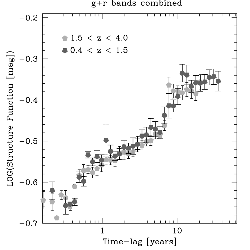
Figure 13: Structure functions for low ($0.4<z<1.5$, dark-gray symbols) and high ($1.5<z<4.0$, light-gray symbols) redshift quasars. The mean redshift for each bin is 1.002 and 2.065, respectively. One would expect that the higher redshift bin is more variable due to the intrinsically bluer part of the spectrum that is probed (cf. Fig. 10). This is not the case, however. The mean offset along the $y$-axis for time-lags beyond 1 year is $\overline{O}=0.011\pm 0.005$.

In the rest of the paper we assume that all the variations are intrinsic to the quasar, and hence the $(1+z)$ time-dilation correction has to be applied. If one wants to consider both the time-dilation corrected and uncorrected cases, one introduces another level of degeneracy between redshift, absolute luminosity, and restframe spectral variability (Hawkins, 2001), which needlessly complicates matters. Based on the results in the last section, we feel confident that the variations are indeed source related.

This brings us to the first of the possible degeneracies: redshift and restframe spectral variability. It is clear that sources vary more in the blue than in the red (cf. Fig. 8, or Giveon et al., 1999; Trevese & Vagnetti, 2002; Hawkins, 2003). Any trend in which higher redshift quasars become intrinsically less variable can be offset against the increase of variability as the observed spectral range shifts toward the blue with increasing redshift. Disentangling the redshift and spectral variability contributions will be difficult, provided the higher redshift SF curve lies above the lower redshift one. However, as is shown in Fig. 13, it is clear that this is not the case: the high-$z$ (light-gray symbols) SF curve lies below the low-$z$ one (dark-gray symbols). This provides us with a solid lower limit on the trend that high-$z$ quasars are less variable than their low-$z$ counterparts.

We measure a mean offset along the $y$-axis of $\overline{O}=0.011\pm 0.005$, for a 2.2$\sigma$ significance. Again, given the intrinsically bluer part of the spectrum that is probed for the high redshift bin ($\overline{z}=2.065$, 18 426 quasars) compared to the low redshift bin ($\overline{z}=1.002$, 18 335 quasars), one expects the former bin to be more variable. That this is not the case only increases the significance of the assessment that low redshift quasars are more variable than high redshift ones.

The observed magnitude range for the quasars between $0.4<z<4.0$ is roughly $18<r<21$ (cf. Fig. 2), and rather uncorrelated with redshift. This in turn implies that the absolute $r_{\mbox{\tiny SDSS}}$-band luminosity (after taking a k-correction into account) of the sample increases as a function of redshift. The two redshift bins of Fig. 13 are therefore also separated in absolute luminosity. Since absolute luminosity is an intrinsic property of the quasar (whereas redshift is not), it makes more sense to investigate the variability as function of absolute luminosity. If one assumes that the quasar variations are similar in an absolute sense, then the relative variations are smaller for the intrinsically brighter objects.

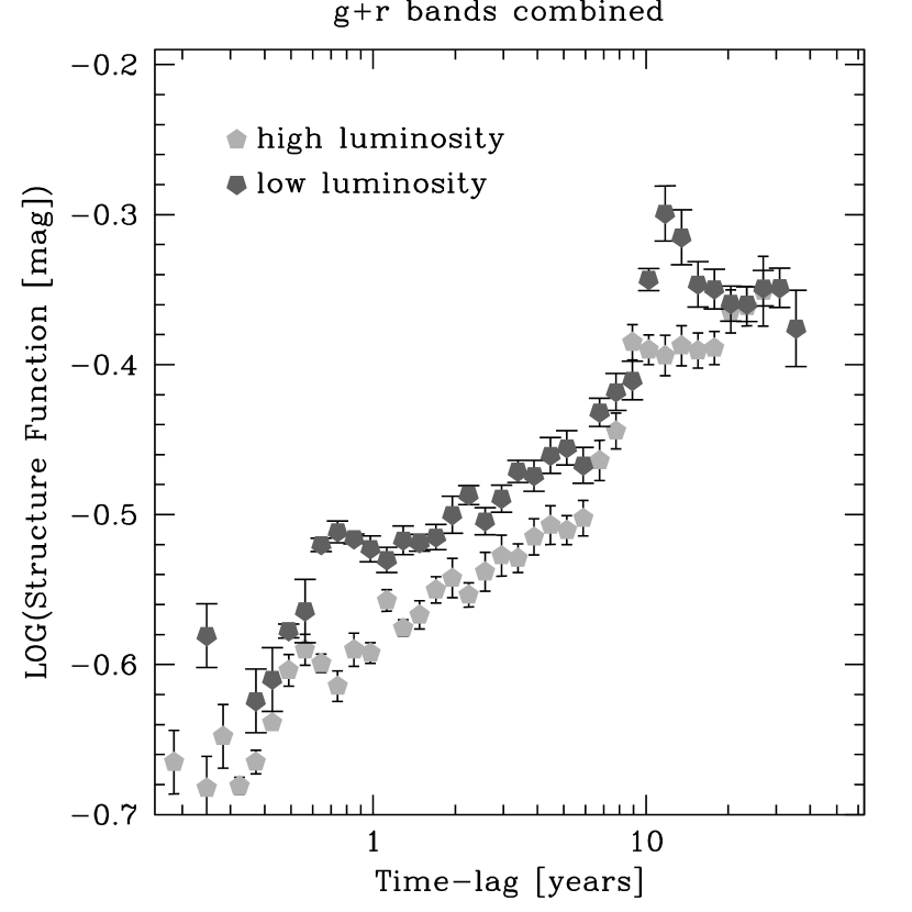
Figure 14: Structure functions for low ($-20>M_{r}>-24.32$, dark-gray symbols) and high ($-24.32>M_{r}>-29$, light-gray symbols) luminosity quasars. The subsample of quasars is identical to the one for Fig. 13, and $M_{r}=-24.32$ represents the mean absolute $r_{\mbox{\tiny SDSS}}$-band luminosity. The offset between the low and high luminosity SF curves is best explained along the $y$-axis, and not the $x$-axis. In other words, the relative variability in low luminosity quasars is larger than in high luminosity quasars, while it does not have a different preferred time-scale.

Figure 14 shows this trend. The subsample of the quasars with redshifts $0.4<z<4.0$ has been divided up into two bins: all the quasars fainter, and brighter than $M_{r}=-24.32$. This value is the mean absolute luminosity of the subsample Note that for the low-luminosity quasars (the dark-gray symbols) the photometry quality degrades toward higher redshifts, which expresses itself as an artificial increase in the SF signal (especially for the time-lags between 10 to 20 years). The GSC2 photometry is less affected by this, resulting in a nicer signal. The SF curves are offset significantly (and more so than in Fig. 13) between time-lags of about a year to $\sim 8$ years.

Based on Figs. 13 and 14, we conclude that high-luminosity quasars vary less than low luminosity quasars. This supports earlier similar findings by, e.g., Hook et al. (1994); Trevese et al. (1994); Cristiani et al. (1996), but contradicts for instance, Giallongo et al. (1991). These authors argued that the absence of the trend for higher luminosity quasars to be less variable points toward a scenario in which the object varies as a single (coherent) source, rather than a flaring sub-unit. Given our results, we have to conclude the opposite, namely that quasars tend to vary incoherently, and do so with a limited magnitude range of the flaring sub-units.

Garcia et al. (1999) tried to explain this within a supernova context (e.g., Aretxaga et al., 1997) in which the time separation between outburst (with total energies of up to $10^{50}$ ergs) are distributed in a Poissonian way. However, the resulting SF curves based on supernovae are too steep (cf. Kawaguchi et al., 1998; Hawkins, 2002), and are effectively ruled out. In Paper I, we applied a similar shot-noise outburst distribution to model the SF curve, but used a broader (more generalized) exponential light-curve. In § 4, we will get back to this issue.

4 Modeling the Structure Function

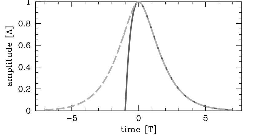
Figure 15: Model light-curves, plotted against time. The asymmetric light-curve is plotted in dark-gray, and is given by Eqn. 5. Its symmetric counterpart is plotted in light-gray (Eqn. 6). The units of time and amplitude have been normalized by $T$ and $A$, respectively. Note that the signal of the asymmetric curve at times $t<-T$ has been set to zero.

In this section we will expand on the modeling done in Paper I. The limited sample size and the resulting noisy SF curve did not allow for accurate fitting in that paper. With the present data, however, we are in a position to investigate this further. The main modeling result from Paper I was that we could approximate the observed SF curve by assuming the following: 1) the typical quasar undergoes periodic outbursts with a decaying time-scale of $\sim 2$ years, and 2) these outbursts occur on a typical time-scale of $\sim 200$ years. As we will see in the next few sections, this simple picture is not correct.

First, let us begin describing the modeling setup we used. Like in Paper I, we assume a typical outburst can be described by a canonical exponential function (Eqn. 5). Curves of these types can be used to model various possible outburst scenarios, ranging from short time-scale supernovae to longer time-scale accretion disk instabilities (see, e.g., Kawaguchi et al., 1998, and references therein). In addition to Paper I, we also introduce a symmetric version of Eqn. 5, given in Eqn. 6. We need both curves to adequately investigate the observed SF asymmetry (cf. § 4.1).

For each equation, $A$ represents the amplitude of the outburst (in magnitudes), $e$ is the normalization constant so that the peak has an amplitude $A$, and $T$ is the exponential half-life time (in years). The time parameter $t$ has been chosen such that the peak of the outburst occurs at time $t=0$. The normalized light-curves have been plotted in Fig. 15 to make this a little clearer. The asymmetric curve (plotted in dark gray) is the exact same as in Paper I, and the symmetric case is identical to the asymmetric one for times $t>0$.

$$L_{\mbox{\small asym}}(t)=eA\left(\frac{t+T}{T}\right)e^{-(t+T)/T}$$ (5)

$$L_{\mbox{\small sym}}(t)=eA\left(\frac{|t|+T}{T}\right)e^{-(|t|+T)/T}$$ (6)

Note that Eqn. 5 is only valid for times $t>-T$. The quantities $A$ and $T$ are free parameters in the model. For each of these points in phase-space, a quasar composite light-curve is constructed covering a large time period (typically 10 000 years). This period is filled up with outbursts based on $A$ and $T$, separated in time by a characteristic outburst time-scale $P$. Like in Paper I, the probability of an outburst not occurring within time $t$ is given by

$$\mbox{Prob($t$)}dt=\left(\frac{1}{P}\right)e^{-t/P}dt$$ (7)

which is also known as a shot noise model of variability (see, e.g., Lochner et al., 1991). Once we have constructed such a canonical quasar light-curve (based on the values of $A$, $T$, and $P$), we generate a database of measurements which is identical to the actual one for our quasars. So we use the very same redshifts (all 41 391), and with on average 4 measurements per quasar (from this canonical light-curve), this results in about 250 000 permutations. This is close to the actual values (170 000 for the $g_{\mbox{\tiny SDSS}}$-band, and 130 000 for the $r_{\mbox{\tiny SDSS}}$-band). To each, randomly sampled, “measurement” we add white noise that matches the actual measurement uncertainties. We adopt the conservative values of $\sigma_{\mbox{\tiny SDSS}}=0.04$, $\sigma_{\mbox{\tiny GSC}}=0.12$, and $\sigma_{\mbox{\tiny POSS}}=0.21$ magnitudes. The error in the magnitude differences are then the rms-values of the appropriate $\sigma$’s. The first two values are in part set by the SF noise plateau at very short time-scales (which do not contain any POSS data), and the $\sigma_{\mbox{\tiny POSS}}$ value is based on the stellar SF plateau in § 3.2.1, which can be considered an upper limit (Sesar et al. (2004) quote a $\sigma=0.15$ mag). The artificial SF curve which is based on these data can then directly be compared to the actual one.

The model SF curve is sampled on the exact same time-lag binning as the actual one, allowing for a simple comparison. There is, however, a complication. The parameter combination of $A$ and $P$ turns out to be degenerate. If one increases the amplitude $A$, and at the same time makes outbursts rarer by increasing the typical time-scale $P$, it results in the same SF curve (which is still dependent on $T$) as for smaller values of $A$ and $P$. The sole thing that discriminates between the two scenarios is that the error-bars in the high $A$, high $P$ case are much larger than in the low $A$, low $P$ case. This can be understood in terms of what defines the typical quasar behavior: in the high $A$, high $P$ case, most quasars will not vary, except for a small subset. This introduces large SF variations, depending on whether such measurements are present in the bin or not. In the low $A$, low $P$ case, a lot of quasars vary, but do so at low amplitude. The relative sample variations are small, and most time-lag bins are made up of more homogeneous measurements. Remember, the error-bars in the SF curves are based on the rms within a set of time-lag bins (we bin bins, see Paper I for more details).

So, instead of a simple $\chi^{2}$ value, our goodness-of-fit is defined by the sum of the $\chi^{2}$ value and the rms in the difference between the sizes of the model and actual error-bars. Their relative values are normalized such that for a good fit each contribution has about equal weight.

The best fitting values of $A$, $T$, and $P$ (or sets thereof in cases where we fit multiple components) are found by exploring the phase-space extensively. Since this space typically does not have any steep gradients, we opted for a slow-cooling simulated annealing code, specifically developed for this purpose. It consistently converged to the same solutions, provided we cooled slow enough.

4.1 Modeling Results

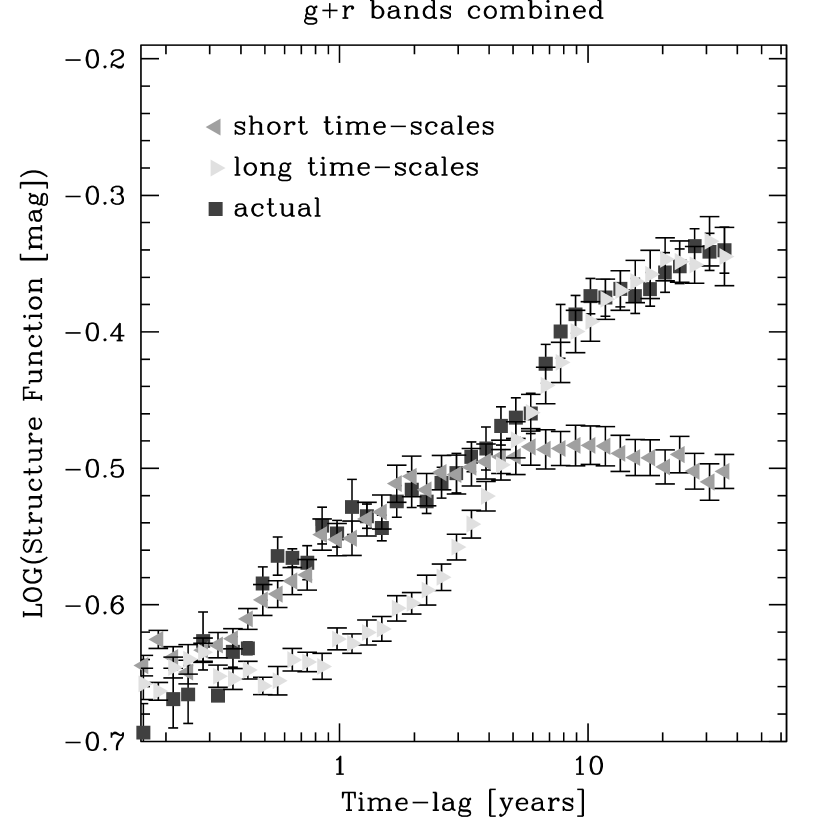
Figure 16: Plot showing the inability to fit the actual SF curve with one single set of $A$, $T$, and $P$ values. Unlike Paper I, where we were able to fit the much poorer data with a single set, this is not possible with the current data. A combination of short- and long-term variability is needed. In this case, separate fits have been made to the actual SF curve: one for time-lags below 5 years, and one for time-lags beyond 5 years.

In the first subsection, we will restrict the modeling to the symmetric light-curve functions (Eqn. 6). After that we are also considering the asymmetric light-curves of Eqn. 5.

4.1.1 Inability to fit single component

In Paper I we were able to fit the observed SF curve adequately by a single set of $ATP$ values, suggesting a possible characteristic variability time-scale / mechanism common to all quasars. The data quality, however, was such that this could not be put on sure footing. With the current high quality data, this is any easy thing to test. As can be seen in Fig. 16, we cannot fit the observed SF curve with a single component. The two model curves, one fitting the short ($<5$ years) time-lags, and one fitting the long ($>5$ years) time-lags illustrate the problem. In order to generate enough signal at the short time-lags, the model light-curve has to have a small half-life $T$. The actual values for the fit are: $A=0.4,T=0.29,P=4$, with $A$ in magnitudes, and $T$, $P$ in years. However, it is also clear that the SF curve belonging to this light-curve does not have any signal increase beyond a few $T$; it effectively levels off after $\sim 3$ years and starts deviating from the actual SF curve significantly. On the other hand, SF model curves that do fit the longer time-lags (based in this case on light-curves with a half-life $T=2.24$ years, $A=0.5$, and $P=18$), do not have any significant SF signal on time-scales much shorter than their $T$ value.

We therefore need at least two variability components. This refutes the notion from Paper I that there is a single preferred variability time-scale common to all quasars. It also implies that there may be a continuum of variability time-scales. Our best fitting two component fit (to the SF curve plotted in Fig. 16) has values of: $A=0.9$, $T=0.27$, $P=23$, and $A=0.5$, $T=3.67$, $P=42$. Again, due to the degeneracy between $A$ and $P$, their values are not very well constrained. Longer periods $P$ are not excluded. However, we did try to make the error-bars on the model SF curve as much like the actual data as possible.

Even fitting with more components did not alter the shortest time-scales. Most of the shortest $T$ values grouped around 0.2 year. Our data have some sensitivity to these short time-lags, but not an awful lot. About 2% of the available time-lag measurements are shorter than 0.2 years. This half-life of up to a few months is comparable to high-redshift supernovae timescales (see, e.g., Barris et al., 2004). The longer time-scales needed to fit the SF curve beyond a few years are more in line with disk instability models of large accretion disks around supermassive black holes (e.g., Kawaguchi et al., 1998). It is therefore not immediately clear what, if any, mechanism dominates.

4.1.2 Modeling SF asymmetries

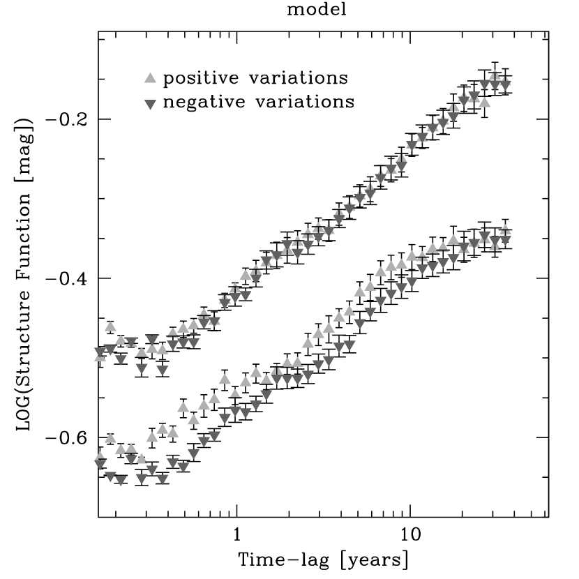
Figure 17: The asymmetry behavior of a particular 3 component model (with half-life values of $T=0.34,T=2.90,T=6.94$, bottom set of data-points), using a light-curve described by Eqn. 5. Even though the combined SF (with both positive- and negative-only variations) fits the observed SF very well, the asymmetry is a bit different from the actual case (Fig. 12): the magnitude of the asymmetry slightly smaller ($\overline{O}=0.022\pm 0.003$), and the “nulls” at $\sim$2 and $\sim$30 year time-lags are not observed either. By comparison, the top set of points (vertically offset by 0.15 for clarity), represents the symmetric case (Eqn. 6) for exactly the same set of parameters and initial random seed. The asymmetry is measured to be $\overline{O}=0.003\pm 0.003$.

As we have seen in § 3.3.6, our quasar SF curve displays significant asymmetry, with a mean offset of $\overline{O}=0.027\pm 0.003$. This is not compatible with our symmetric fits from the previous section, which consistently resulted in offsets of $\overline{O}\approx 0.000$, to within the $0.003$ uncertainty (cf. Fig. 17, top curve). Hence, we need to introduce some measure of light-curve asymmetry into our modeling. For this, we use Eqn. 5 as the functional form of the light-curve.

The fitting method is the same as for the symmetric light-curve case, and the results are reasonably comparable. Given the shape of the light-curves (cf. Fig. 15), one expects to find larger values of $T$ for the asymmetric case than for the symmetric one. This is because the latter light-curve has variations at longer time-scales than the asymmetric one for identical values of $T$.

We find for the asymmetric 2 component case: $A=0.8$, $T=0.45$, $P=23$, and $A=0.5$, $T=5.43$, $P=42$, which has indeed larger values of $T$ than the symmetric case. It also carries the asymmetry signal we are interested in. A typical resulting SF is shown in Fig. 17, separated into negative- and positive-only variations. The SF curves are clearly separated (mean offset $\overline{O}=0.022\pm 0.003$ for this case). However, there are a few things that are not entirely consistent with the observed data. Aside from the slightly smaller value of the asymmetry signal $\overline{O}$, it appears that for time-lags somewhat shorter than $T$, the SF does not have an asymmetry signal. This is not observed in the actual data (cf. Fig. 12). Since these nulls are associated with the few discrete time-scales $T$, adding in more intermediate $T$’s will smooth out and remove the nulls. This suggests that the intrinsic quasar variations have a more continuous distribution of $T$’s. Indeed, our models with more than four components tend not to have these nulls.

The data, and our modeling effort, do not allow for a precise characterization of the magnitude of the light-curve asymmetry. It also does not allow for the isolation of particular variability time-scales, and is more compatible with a scenario in which quasars can vary with a continuous distribution of time-scales. One thing that is clear, though, is that the variations are asymmetric, and are of the fast-rise, slow-decline type.

4.1.3 Estimating intrinsic SF slope

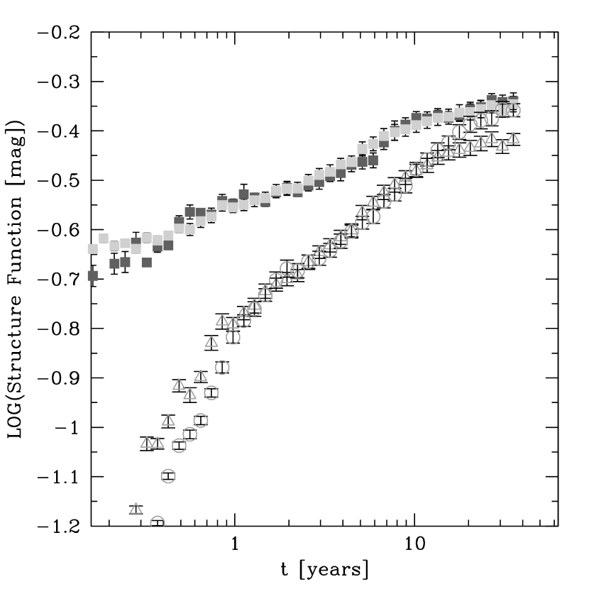
Figure 18: SF slope changes due to removal of measurement noise. The top two sets of points represent the actual SF and best fitting 3 component model (same as in Fig. 17). Note that the y-axis scale has been expanded. The slope of these curves is $\alpha=0.15\pm 0.01$. The bottom 2 sets of points represent the SF for the exact same 3 component model, but with the magnitude measurement noise for the SDSS, GSC, and POSS surveys set to zero. The triangles and circles are for the asymmetric and symmetric light-curves respectively. The slopes for both SFs are $\alpha=0.30\pm 0.01$, at least for the flat part between time-lags of 1 to 20 years.

The theoretical slope calculations in Kawaguchi et al. (1998) do not include a white noise component, as their data quality for the individual sources was good enough. We, however, do have to include a white noise term in our modeling to make it agree with the actual data better. This does have the side-effect of lowering the SF slope (as noted in Paper I), which potentially might render the slope comparison suspect. To this end, we have generated “noise-less” SF curves derived from a well fitting “noise-included” SF curve. The results have been plotted in Fig. 18. The top set of data-points are the actual SF with the best fitting (3 component in this case) SF model. The slope for both curves is measured to be $0.15\pm 0.01$, which, as discussed in § 3.3.4, is much shallower than any of the Kawaguchi et al. (1998) values. If we remove the measurement noise components, we end up with the two bottom sets of SF curves (a symmetric and an asymmetric one). Note that even though there is no measurement noise present, there will always be a range of magnitude differences for a fixed time-lag (unless there is no variation), which explains the presence of error-bars.

The slope for these curves is measured to be $\alpha=0.30\pm 0.01$, which indeed is steeper. The fall-off below time-lags of a year is due to the fact that the actual SF (top curve in the figure) does not have any sensitivity to these short time-scales, as they are effectively masked by the measurement noise. Since we just de-noised the fit to the actual SF, this lack of short time-scale signal becomes apparent. The quoted slope, therefore, is only for the SF curve beyond time-lags of one year.

While the slope of the SF has indeed steepened a bit in the noise-less case, it is not enough to change the assessment of § 3.3.4 in a significant way. It is still too shallow for either the SB or DI models, but is now marginally steeper than the micro-lensing slope.

5 Discussion and Summary

Our results on the quasar SF strongly suggest, for the first time, that most of the long-term variations are intrinsic to the quasar itself. Micro-lensing by objects along the line-of-sight to the quasar, or even in the quasar host galaxy itself, is not a viable explanation of the long-term variability in general.

This result is mainly based on the observed asymmetry in the SF, indicative of a fast-rise, slow-decline type of variability (cf. § 3.3.6). The significance of the observed asymmetry is enhanced by the Malmquist signal, which works in the opposite sense. If our measured asymmetry would have had the same sign as the Malmquist bias, one would be hard pressed to ascribe any of that asymmetry to the intrinsic quasar variability behavior, and the data would have been consistent with the symmetric variations needed in the micro-lensing scenario. This is, however, not the case. The formal statistical significance of the asymmetry is $6\sigma$.

We have put some other results on a more secure footing as well. First, no obvious turnover has been detected in the quasar SF, which indicates that there is no upper preferred variability time-scale (smaller than a few decades). Our results are consistent with a continuum range of variation time-scales. This is based on the absence of a turnover, as well as on the near constant offset between positive- and negative-only variations in Fig. 10. If we model asymmetry based on a few preferred time-scales $T$, we find almost no asymmetry signal at timescales of a few times $T$ (cf. Fig. 17), something clearly absent in the real data. A more or less constant offset in the model can be achieved with a larger number of components (4 or more), all with time-scales $T$ less than 10 years. This opens up the door to any number of components, since as far as we know there is no observed turnover beyond $\sim$40 years which would set an upper bound.

Second, the magnitude of the quasars variability is a clear function of wavelength: variability increases toward the blue part of the spectrum. This confirms previous observations by, e.g., Giallongo et al. (1991); Giveon et al. (1999); Trevese & Vagnetti (2002); Hawkins (2003), and is consistent with both the starburst (SB) and the disk instability (DI) model of variability. However, based on the model SF slopes by Kawaguchi et al. (1998), the SF slopes for the SB model $(0.74<\alpha<0.90$) are even more inconsistent with our “noise-less” modeled value of $(\alpha=0.30\pm 0.01)$ than the DI values of $(0.41<\alpha<0.49)$. Clearly, some modifications need to be made before the models can adequately describe the observations.

Third, high-luminosity quasars vary less than low-luminosity quasars. This is consistent with a scenario in which variations have a limited absolute magnitude, and variations are due to sub-components instead of coherent variation of the AGN (e.g., Garcia et al., 1999). These sub-components can be interpreted as either individual supernovae, or discrete flares due to disk instabilities.

In summary, all the data presented here lead to the conclusion that quasar variability is intrinsic to the source, is caused by chromatic outbursts / flares with limited luminosity range and varying time-scales, and with an overall asymmetric light-curve. Currently, the model that best explains this observed behavior is based on accretion disk instabilities. However, given the existing discrepancies between the SF slopes of the model and observations, some reservations are still in place.

References

- Abazajian et al. (2004) Abazajian, K., Adelman-McCarthy, J. K., et al. 2004, ApJ, in press (astro-ph/04033425)
- Alexander (1995) Alexander, T. 1995, MNRAS, 274, 909
- Aretxaga et al. (1997) Aretxaga, I., Cid Fernandes, R., & Terlevich, R. J. 1997, MNRAS, 286, 271
- Bahcall & Soneira (1980) Bahcall, J. N., & Soneira, R. M. 1980, ApJS, 44, 73
- Bahcall & Soneira (1981) Bahcall, J. N., & Soneira, R. M. 1981, ApJ, 246, 122
- Barris et al. (2004) Barris, B. J., Tonry, J. L., et al. 2004, ApJ, 602, 571
- Becker et al. (1995) Becker, R. H., White, R. L., & Helfand, D. J. 1995, ApJ, 450, 559
- Bregman et al. (1990) Bregman, J. N., Glassgold, A. E., Huggins, P. J., et al. 1990, ApJ, 352, 574
- Cid Fernandes et al. (1996) Cid Fernandes, R., Aretxaga, I., & Terlevich, R. 1996, MNRAS, 282, 1191
- Cid Fernandes et al. (2000) Cid Fernandes, R., Sodré Jr, L., & Vieira da Silva Jr, L. 2000, ApJ, 544, 123
- Cristiani et al. (1996) Cristiani, S., Trentini, S., La Franca, F., Aretxaga, I., Andreani, P., Vio, R., & Gemmo, A. 1996, A&A, 306, 395
- Croom et al. (2004) Croom, S. M., Smith, R. J., Boyle, B. J., Shanks, T., Miller, L., & Outram, P. J. 2004, MNRAS, in press (astro-ph/0403040)
- Derue et al. (2002) Derue, F., Marquette, J-B., Lupone, S., et al. 2002, A&A, 389, 149
- de Vries, Becker & White (2003) de Vries, W. H., Becker, R. H., & White, R. L. 2003, AJ, 126, 1217
- Eggers et al. (2000) Eggers, D., Shaffer, D. B., & Weistrop, D. 2000, AJ, 119, 460
- Enya et al. (2002a) Enya, K., Yoshii, Y., Kobayashi, Y., Minezaki, T., Suganuma, M., Tomita, H., & Peterson, B. A. 2002, ApJS, 141, 31
- Enya et al. (2002b) Enya, K., Yoshii, Y., Kobayashi, Y., Minezaki, T., Suganuma, M., Tomita, H., & Peterson, B. A. 2002, ApJS, 141, 45
- Fan & Lin (2000) Fan, J. H., & Lin, R. G., 2000, ApJ, 537, 101
- Gal et al. (2003) Gal, R. R., de Carvalho, R. R., Odewahn, S. C., Djorgovski, S. G., Mahabal, A., Brunner, R. J., & Lopes, P. 2003, AJ, 125, 2064
- Garcia et al. (1999) Garcia, A., Sodré Jr, L., Jablonski, F. J., & Terlevich, R. J. 1999, MNRAS, 309, 803
- Giallongo et al. (1991) Giallongo, E., Trevese, D., & Vagnetti, F. 1991, ApJ, 377, 345
- Giveon et al. (1999) Giveon, U, Maoz, D., Kaspi, S., Netzer, H., & Smith, P. S. 1999, MNRAS, 306, 637
- Hawkins (1993) Hawkins, M. R. S. 1993, Nature, 366, 424
- Hawkins (1996) Hawkins, M. R. S. 1996, MNRAS, 278, 787
- Hawkins (2001) Hawkins, M. R. S. 2001, ApJ, 553, L97
- Hawkins (2002) Hawkins, M. R. S. 2002, MNRAS, 329, 76
- Hawkins (2003) Hawkins, M. R. S. 2003, MNRAS, 344, 492
- Hook et al. (1994) Hook, I. M., McMahon, R. G., Boyle, B. J., & Irwin, M. J. 1994, MNRAS, 268, 305
- Hughes et al. (1992) Hughes, P. A., Aller, H. D., & Aller, M. F. 1992, ApJ, 396, 469
- Kawaguchi et al. (1998) Kawaguchi, T., Mineshige, S., Unemara, M., & Turner, E. L. 1998, ApJ, 504, 671
- Lattanzi & Bucciarelli (1991) Lattanzi, M. G. & Bucciarelli, B. 1991, A&A, 250, 565
- Lochner et al. (1991) Lochner, J. C., Swank, J. H., & Szymkowiak, A. E. 1991, ApJ, 376, 295
- McLean et al. (1998) McLean, B. J., Hawkins, G., Spagna, A., Lattanzi, M., Lasker, B. M., Jenkner, H., & White, R. L. 1998, “The Second Guide Star Catalogue”, in “New Horizons from Multi-Wavelength Sky Surveys”, proceedings of IAU Symposium 179, eds. B. McLean, D. Golombek, J. Hayes, & H. Payne, p. 431
- Monet et al. (2003) Monet, D. G., Levine, S. E., Canzian, B., et al. 2003, AJ, 125, 984
- Rees (1984) Rees, M. J. 1984, ARA&A, 22, 471
- Reid et al. (1991) Reid I. N., Brewer, C., Brucato, R. J., et al. 1991, PASP, 103, 661
- Richards et al. (2002) Richards, G. T., Fan, X., Newberg, H. J., et al. 2002, AJ, 123, 2945
- Sesar et al. (2004) Sesar, B., Svilkovic, D., Ivezic, Z., et al. 2004, ApJ, in press (astro-ph/0403319)
- Shakura & Sunyaev (1976) Shakura, N. I., & Sunyaev, R. A. 1976, MNRAS, 175, 613
- Siemiginowska & Elvis (1997) Siemiginowska, A., & Elvis, M. 1997, ApJ, 482, L9
- Starling et al. (2004) Starling, R. L. C., Siemiginowska, A., Uttley, P., & Soria, R. 2004, MNRAS, 347, 67
- Stoughton et al. (2002) Stoughton, C., Lupton, R., et al. 2002, AJ, 123, 485
- Terlevich et al. (1992) Terlevich, R., Tenorio-Tagle, G., Franco, J., & Melnick, J. 1992, MNRAS, 255, 713
- Trevese et al. (1994) Trevese, D., Kron, R. G., Majewski, S. R., Bershady, M. A., & Koo, D. C. 1994, ApJ, 433, 494
- Trevese & Vagnetti (2002) Trevese, D., & Vagnetti, F. 2002, ApJ, 564, 624
- Ulrich, Maraschi & Urry (1997) Ulrich, M-H., Maraschi, L., & Urry, C. M. 1997, ARA&A, 35, 445
- Vagnetti et al. (2003) Vagnetti, F., Trevese, D., & Nesci, R. 2003, ApJ, 590, 123
- Vanden Berk et al. (2004) Vanden Berk, D. E., Wilhite, B. C., Kron, R. G., et al. 2004, ApJ, 601, 692
- Yonehara et al. (1999) Yonehara, A., Mineshige, S., Fukue, J., Umemura, M., & Turner, E. L. 1999, A&A, 343, 41
- Zackrisson et al. (2003) Zackrisson, E., Bergvall, N., Marquart, T., & Helbig, P. 2003, A&A, 408, 17