Cosmological weak lensing with the HST GEMS survey

Abstract

We present our cosmic shear analysis of GEMS, one of the largest wide-field surveys ever undertaken by the Hubble Space Telescope. Imaged with the Advanced Camera for Surveys (ACS), GEMS spans 795 square arcmin in the Chandra Deep Field South. We detect weak lensing by large-scale structure in high resolution F606W GEMS data from $\sim 60$ resolved galaxies per square arcminute. We measure the two-point shear correlation function, the top-hat shear variance and the shear power spectrum, performing an E/B mode decomposition for each statistic. We show that we are not limited by systematic errors and use our results to place joint constraints on the matter density parameter $\Omega_{m}$ and the amplitude of the matter power spectrum $\sigma_{8}$. We find $\sigma_{8}(\Omega_{m}/0.3)^{0.65}=0.68\pm 0.13$ where the $1\sigma$ error includes both our uncertainty on the median redshift of the survey and sampling variance.

Removing image and point spread function (PSF) distortions are crucial to all weak lensing analyses. We therefore include a thorough discussion on the degree of ACS PSF distortion and anisotropy which we characterise directly from GEMS data. Consecutively imaged over 20 days, GEMS data also allows us to investigate PSF instability over time. We find that, even in the relatively short GEMS observing period, the ACS PSF ellipticity varies at the level of a few percent which we account for with a semi-time dependent PSF model. Our correction for the temporal and spatial variability of the PSF is shown to be successful through a series of diagnostic tests.

1 Introduction

Weak gravitational lensing is a unique probe of the dark matter distribution at redshifts $z<1$ where, within the currently favoured $\Lambda$CDM cosmological paradigm, dark energy begins to play an important role in the evolution and growth of the power spectrum of matter fluctuations. It therefore not only has the power to constrain fundamental cosmological parameters such as the matter density parameter $\Omega_{m}$ and the amplitude of the matter power spectrum $\sigma_{8}$ (Maoli et al., 2001; Rhodes et al., 2001; Van Waerbeke et al., 2001; Hoekstra et al., 2002; Bacon et al., 2003; Jarvis et al., 2003; Brown et al., 2003; Hamana et al., 2003; Massey et al., 2004; Rhodes et al., 2004; Van Waerbeke et al., 2005), but also has the potential to test and constrain quintessence models parameterised by the equation of state of the dark energy ${\rm w}(z)$ (Refregier et al., 2004; Jarvis et al., 2005). Cosmological parameter constraints from weak lensing analysis are fully complementary to those from cosmic microwave background (CMB) experiments as parameter degeneracies are almost orthogonal in many cases (Brown et al., 2003; Contaldi et al., 2003; Tereno et al., 2005). Alone, measurements of the CMB anisotropy at $z\sim 1000$ are unable to constrain ${\rm w}(z)$ but combined with future wide-field weak lensing surveys, potentially focused on selected galaxy clusters (Jain & Taylor, 2003), the goal of determining ${\rm w}(z)$ will certainly become attainable.

Lensing by large-scale structure distorts images of background galaxies, inducing weak correlations in the observed ellipticities of galaxies, termed ‘cosmic shear’. The amplitude and angular dependence of these correlations are related to the non-linear matter power spectrum $P_{\delta}(\ell)$ and the geometry of the Universe. If we first assume that the minute weak lensing shear distortions can be measured in the absence of any systematic errors, arising for example from telescope and detector based distortions, the error on any weak lensing analysis then has four main sources: shot noise from the intrinsic ellipticity distribution of galaxies, sampling (cosmic) variance, uncertainty in the galaxy redshift distribution and uncertainty in intrinsic correlations that may exist between nearby galaxy pairs. Shot noise can be minimised by surveying large areas of sky and/or by increasing the number density of resolved galaxies in the weak lensing analysis. Sampling variance can be minimised by imaging many different lines of sight. With spectroscopic or photometric redshift information the galaxy redshift distribution can be accurately estimated (Brown et al., 2003; Van Waerbeke et al., 2005). Redshift information also allows for the removal of intrinsic correlations (King & Schneider, 2002; Heymans & Heavens, 2003; Heymans et al., 2004). This effect has however been shown to be a small contaminant to the weak lensing signal measured from deep surveys (median redshift $z_{m}\sim 1.0$), at the level of less than a few percent of the shear correlation signal (Heymans et al., 2004). The next generation of weak lensing surveys aim to obtain precise results, minimising these sources of error by surveying of the order of a hundred square degrees with accompanying photometric redshift information. These ground-based surveys are however subject to atmospheric seeing which erases the weak lensing shear information from all galaxies smaller than the size of the seeing disk. This, in effect, limits the maximum depth of ground-based weak lensing surveys and hence the sensitivity, leading to proposals for future deep wide-field space-based observations (Rhodes et al., 2004). With space-based data the number density of resolved galaxies, in comparison to ground-based studies, is multiplied two-fold and more. Resolving images of more distant galaxies will permit high resolution maps of the dark matter distribution (Massey et al., 2004) and will yield significantly higher signal-to-noise constraints on cosmological parameters in comparison to constraints obtained from the same survey area of a seeing limited ground-based survey (Brown et al. in prep).

With the installation of the Advanced Camera for Surveys (ACS) on the Hubble Space Telescope (HST), relatively wide-field space-based weak lensing studies are feasible and in this paper we present the detection of weak gravitational lensing by large-scale structure in GEMS; the Galaxy Evolution from Morphology and Spectral energy distributions survey (see Rix et al. 2004 for an overview). Spanning $795$ square arcmin, GEMS is currently the largest space-based colour mosaic. With a high number density of resolved sources and spectroscopic and/or photometric redshifts for $\sim 8000$ of our sources from the COMBO-17 survey (Wolf et al., 2004) and the VVDS (Le Fèvre et al., 2004), we can beat down shot noise and obtain a good estimate of the galaxy redshift distribution.

The error sources discussed above have not included systematic errors, but in reality for all weak lensing surveys the accuracy of any analysis depends critically on the correction for instrumental distortions, which are orders of magnitude larger than the underlying gravitational shear distortions that we wish to detect. The strongest distortion results from a convolution of the image with the point spread function (PSF) of the telescope and camera. For the detection of cosmic shear at the level of only a few percent, the PSF distortion needs to be understood and controlled to an accuracy of better than one percent. For space-based weak lensing studies (Hoekstra et al., 1998; Rhodes et al., 2000, 2001; Refregier et al., 2002; Hämmerle et al., 2002; Casertano et al., 2003; Rhodes et al., 2004; Miralles et al., 2005), the limited number of stars in each camera field of view provides insufficient coverage to map the PSF anisotropy. This has made it necessary to assume long-term stability in the PSF pattern, often using PSF models derived from archived images of globular clusters, with low order focus corrections, or from Tiny Tim (Krist, 2000) thereby critically limiting the accuracy of the correction for PSF distortions. In contrast to previous space-based lensing studies we are not forced to assume long-term PSF stability as the GEMS PSF can be characterised directly from the wide-area data where all but three out of the sixty-three ACS images were observed in the space of 20 days. Hence we need only assume short term PSF stability, which we test in Section 4.1. A detailed investigation into the GEMS ACS PSF will be presented in Jahnke et al. (in prep) with a view to many different astronomical applications.

This paper is organised as follows. In Section 2 we summarise the basic theory that underpins cosmic shear studies and review the particulars of our analysis. We discuss, in Section 3, the observations and data reduction, paying specific attention to potential sources of image distortions. We focus on characterising and correcting for the temporally and spatially varying dominant PSF distortion in Section 4 and compare, in Section 5, galaxy shear measured from the two GEMS passbands; F606W and F850LP. In Section 6 we estimate the redshift distribution of the GEMS survey from COMBO-17 and VVDS redshift catalogues. Our statistical analysis is detailed in Section 7 where we measure the shear correlation function, the top-hat shear variance statistic and the shear power spectrum performing many diagnostic tests for systematic errors. These results are used to place joint constraints on $\Omega_{m}$ and $\sigma_{8}$ in Section 8. We conclude in Section 9 with a comparison to results from other space-based and ground-based cosmic shear analyses.

2 Method

The theory of weak gravitational lensing by large structure, detailed in Bartelmann & Schneider (2001), directly relates the non-linear matter power spectrum $P_{\delta}$ to the observable weak lensing (complex) shear field $\gamma=\gamma_{1}+i\gamma_{2}$ characterised through the shear (convergence) power spectrum $P_{\kappa}$,

$$P_{\kappa}(\ell)=\frac{9H_{0}^{4}\Omega_{m}^{2}}{4c^{4}}\int_{0}^{w_{H}}dw\,\frac{g^{2}(w)}{a^{2}(w)}\,P_{\delta}\left(\frac{\ell}{f_{K}(w)},w\right),$$ (1)

where $w$ is the comoving radial distance, $a(w)$ is the dimensionless scale factor, $H_{0}$ is the Hubble parameter, $\Omega_{m}$ the matter density parameter and $g(w)$ is a weighting function locating the lensed sources,

$$g(w)=\int_{w}^{w_{H}}\,dw^{\prime}\ \phi(w^{\prime})\frac{f_{K}(w^{\prime}-w)}{f_{K}(w^{\prime})},$$ (2)

where $\phi\left[w(z)\right]dw$ is the observed number of galaxies in $dw$ and $w_{H}$ is the horizon distance (Schneider et al., 1998). Note in this paper we will assume a flat Universe with zero curvature where the comoving angular diameter distance $f_{K}(w)=w$.

In this paper we measure directly the shear power spectrum $P_{\kappa}$, the shear correlation function $\langle\gamma(\mbox{\boldmath{$\theta$}})\gamma(\mbox{\boldmath{$\theta$}}+\Delta\theta)\rangle$ which we split into a tangential component

$$\langle\gamma_{t}\gamma_{t}\rangle_{\theta}=\frac{1}{4\pi}\int d\ell\,\ell\,P_{\kappa}(\ell)\,[J_{0}(\ell\theta)+J_{4}(\ell\theta)],$$ (3)

and a rotated component

$$\langle\gamma_{r}\gamma_{r}\rangle_{\theta}=\frac{1}{4\pi}\int d\ell\,\ell\,P_{\kappa}(\ell)\,[J_{0}(\ell\theta)-J_{4}(\ell\theta)],$$ (4)

and the top-hat shear variance $\langle|\gamma|^{2}\rangle_{\theta}$ measured in a circle of angular radius $\theta$

$$\langle\gamma^{2}\rangle_{\theta}=\frac{1}{2\pi\theta^{2}}\int\frac{d\ell}{\ell}\,P_{\kappa}(\ell)\,[J_{1}(\ell\theta)]^{2}\,.$$ (5)

Note $J_{i}$ is the $i^{\rm th}$ order Bessel function of the first kind.

In order to exploit the straightforward physics of weak lensing, one requires an estimate of the gravitational shear experienced by each galaxy. Kaiser et al. (1995), Luppino & Kaiser (1997) and Hoekstra et al. (1998) (KSB+) prescribe a method to invert the effects of the PSF smearing and shearing, recovering an unbiased shear estimator uncontaminated by the systematic distortion of the PSF. Objects are parameterised according to their weighted quadrupole moments

$$Q_{ij}=\frac{\int\,d^{2}\theta\,W(\mbox{\boldmath{$\theta$}})\,I(\mbox{\boldmath{$\theta$}})\,\theta_{i}\theta_{j}}{\int d^{2}\theta\,W(\mbox{\boldmath{$\theta$}})\,I(\mbox{\boldmath{$\theta$}})},$$ (6)

where $I$ is the surface brightness of the object, $\theta$ is the angular distance from the object centre and $W$ is a Gaussian weight function of scale length $r_{g}$, where $r_{g}$ is some measurement of galaxy size, for example the half light radius. For a perfect ellipse, the weighted quadrupole moments are related to the weighted ellipticity parameters $\varepsilon_{\alpha}$ by

$$\left(\begin{array}[]{c}\varepsilon_{1}\\ \varepsilon_{2}\end{array}\left)=\frac{1}{Q_{11}+Q_{22}}\right(\begin{array}[]{c}Q_{11}-Q_{22}\\ 2Q_{12}\end{array}\right).$$ (7)

Kaiser et al. (1995) show that if the PSF distortion can be described as a small but highly anisotropic distortion convolved with a large circularly symmetric seeing disk, then the ellipticity of a PSF corrected galaxy is given by

$$\varepsilon^{\rm cor}_{\alpha}=\varepsilon^{\rm obs}_{\alpha}-P^{\rm sm}_{\alpha\beta}p_{\beta},$$ (8)

where $p$ is a vector that measures the PSF anisotropy, and $P^{\rm sm}$ is the smear polarisability tensor given in Hoekstra et al. (1998). $p(\mbox{\boldmath{$\theta$}})$ can be estimated from images of stellar objects at position $\theta$ by noting that a star, denoted throughout this paper with ^∗, imaged in the absence of PSF distortions has zero ellipticity: $\varepsilon^{*\,{\rm cor}}_{\alpha}=0$. Hence,

$$p_{\mu}=\left(P^{\rm sm*}\right)_{\mu\alpha}^{-1}\,\varepsilon^{*{\rm obs}}_{\alpha}.$$ (9)

For space-based imaging, where PSFs deviate strongly from a Gaussian, this PSF correction is mathematically poorly defined (Kaiser, 2000) such that it is important to calculate the PSF correction vector $p$ not only as a function of galaxy position $\theta$, but also as a function of galaxy size $r_{g}$ (Hoekstra et al., 1998). This rather unsatisfactory situation has prompted the development of alternative methods (Rhodes et al., 2000; Kaiser, 2000; Bernstein & Jarvis, 2002; Refregier & Bacon, 2003; Massey & Refregier, 2004) but for the purpose of this paper we will focus on the most commonly used KSB+ technique, deferring our analysis with different techniques to a future paper.

The isotropic effect of the PSF is to convolve galaxy images with a circular kernel. This makes objects appear rounder, erasing shear information for galaxies smaller than the kernel size, which have to be removed from the galaxy shear sample. For the larger galaxies, this resolution effect can be accounted for by applying the pre-seeing shear polarisability tensor correction $P^{\gamma}$, as proposed by Luppino & Kaiser (1997), such that

$$\varepsilon^{\rm cor}_{\alpha}=\varepsilon^{s}_{\alpha}+P^{\gamma}_{\alpha\beta}\gamma_{\beta}.$$ (10)

where $\varepsilon^{s}$ is the true source ellipticity and $\gamma$ is the pre-seeing gravitational shear. Luppino & Kaiser (1997) show that

$$P^{\gamma}_{\alpha\beta}=P^{\rm sh}_{\alpha\beta}-P^{\rm sm}_{\alpha\mu}\left(P^{\rm sm*}\right)_{\mu\delta}^{-1}P^{\rm sh*}_{\delta\beta},$$ (11)

where $P^{\rm sh}$ is the shear polarisability tensor given in Hoekstra et al. (1998) and $P^{\rm sm*}$ and $P^{\rm sh*}$ are the stellar smear and shear polarisability tensors respectively. This relation is only strictly true when all values are measured from the PSF de-convolved image which is difficult to create in practice. $P^{\gamma}$ is therefore calculated from the PSF distorted images which produces very noisy measurements.

Combining the PSF correction, equation (8), and the $P^{\gamma}$ seeing correction, the final KSB+ shear estimator $\hat{\gamma}$ is given by

$$\hat{\gamma}_{\alpha}=\left(P^{\gamma}\right)^{-1}_{\alpha\beta}\left[\varepsilon^{\rm obs}_{\beta}-P^{\rm sm}_{\beta\mu}p_{\mu}\right].$$ (12)

When averaging over many galaxies, assuming a random distribution of intrinsic galaxy ellipticities, $\langle\varepsilon^{s}\rangle=0$, and hence $\langle\hat{\gamma}\rangle=\gamma$, providing a good estimate for the gravitational shear.

3 The GEMS data

The GEMS survey (Rix et al., 2004) spans an area of $\sim 28^{\prime}\times 28^{\prime}$ centred on the Chandra Deep Field South (CDFS), combining 125 orbits of ACS/HST time with supplementary data from the GOODS project (Giavalisco et al., 2004). 78 ACS tiles have been imaged in F606W and 77 ACS tiles in F850LP, where the point source $5\sigma$ detection limits reach ${\rm m}_{606}=28.3$ and ${\rm m}_{850}=27.1$. In this section we review the data set, discuss the potential for bias within the source catalogues and highlight possible sources of image distortion, in addition to the strong anisotropic PSF distortion which is characterised and corrected for in Section 4. A detailed account of the full GEMS data reduction method will be presented by Caldwell et al. (in prep).

The ACS wide-field camera has a field-of-view $\sim 3.4\times 3.4$ arcmin comprising two $4096\times 2048$ CCD chips of pixel scale $0.05$ arcsec (Ford et al., 2003). GEMS observes, in sequence, three separate exposures per ACS tile dithered by $\sim 3$ arcsec, where the observation strategy has been designed in such a way so as to bridge the inter-chip gap and provide sub-pixel oversampling of pixel scale $0.03$ arcsec in the final co-added image ($\sim 7000\times 7000$ pixels). GOODS have employed a different observing strategy, using only two separate dithered exposures. In order to optimise the survey for Supernova searches (Riess et al., 2004) the GOODS area is re-imaged in 5 different epochs, but to obtain similar depths to the GEMS data and minimise the effects of PSF time variation, we co-add only the exposures from the first epoch of observations. This however leaves us with a slightly shallower central region in the F606W GEMS mosaic which can be seen from the median magnitude of each data set; ${\rm m}_{606}({\rm GEMS})=25.6$, ${\rm m}_{606}({\rm GOODS})=25.1$. We note that the 2 exposure GOODS dithering pattern will result in a poorer cosmic ray rejection in the GOODS area of the GEMS mosaic, and will impact somewhat on the PSF.

Images from the ACS suffer from strong geometric distortions as a result of the off-axis location of the camera within HST. In addition, the HST optical assembly and the ACS mirrors also induce distortions. Meurer et al. (2003) accurately calibrate and model this distortion from dithered images of star clusters. With this model all tiles are drizzled onto a celestial pixel grid using a version of the multidrizzle software (Koekemoer et al., 2003), where the astrometry of each GEMS tile is tied to the overall catalogue from the ground-based COMBO-17 $R$ band image (Wolf et al., 2004). Averaging our final PSF corrected shear catalogues as a function of ACS chip position, we find no evidence for any residual geometric distortions remaining in our final multi-drizzled images.

A second order geometric distortion arises from the effect of velocity aberration (Cox & Gilliland, 2002). The HST guides on nearby stars peripheral to the ACS field of view, making small corrections to keep the primary target on a fixed pixel. It cannot however correct for the isotropic plate-scale breathing which is of the order $\sim 0.001\%$ over an orbit. These small changes in pixel scale are allowed for and corrected by our version of multidrizzle, provided the individual exposures are on the same scale. Variation of scale during each observation would result in a slight blurring of the co-added images that increases radially from the centre. GEMS ACS tiles, observed over 1/7 of the orbit, suffer from pixel scale variation that is, at maximum, a difference of $0.004$ arcsec corner to corner. Our results later show no significant variation in average galaxy shear as a function of chip position and we hence conclude that this effect is not significant within our measurement accuracy. In future data reductions of GEMS we will include a velocity aberration correction to the pixel scale using an updated version of multi-drizzle.

We use the SExtractor software (Bertin & Arnouts, 1996) to detect sources on both the F606W and F850LP imaging data, with the two-step approach described in Rix et al. (2004). In short, this method of combining two SExtractor catalogues, one measured with high signal-to-noise detection thresholding, and one measured with low signal-to-noise detection thresholding, allows us to find the best compromise between detecting faint galaxies without deblending bright nearby galaxies into many different components. We also use SExtractor to determine the weak variation of the sky background across the tile, which is then subtracted for the following KSB+ analysis. We define galaxy size $r_{g}$ as the half light radius measured by SExtractor (flux_radius) and calculate weighted ellipticity parameters $\varepsilon_{i}$ and the shear and smear polarisability tensors; $P^{\rm sh}$ and $P^{\rm sm}$ for each object in the SExtractor catalogue.

The accuracy of the centroid determined by SExtractor is directly linked to the accuracy of each KSB+ galaxy shear measurement. In the presence of non-isotropic centroiding errors there is also the potential for centroid bias (Kaiser, 2000; Bernstein & Jarvis, 2002) which can arise if, for example, the errors in the $x$ direction exceed those in the $y$ direction producing a tendency to bias towards an average galaxy shear in the $x$ direction. The GEMS galaxies have been modelled using the two-dimensional galaxy profile model fitting code GALFIT (Peng et al., 2002) which finds the best fit PSF convolved Sérsic profiles to each galaxy, allowing the centroid to be a free parameter in the fit (see Barden et al. 2004 and Häußler et al. in prep for details). We can therefore test if we are subject to centroid bias by comparing GALFIT and SExtractor centroids. The average pixel offset is consistent with zero in the $x$ direction, $\Delta x=-0.001\pm 0.02$ and very close to zero in the $y$ direction $\Delta y=0.03\pm 0.02$. Calculating the ellipticity of a mock circular Gaussian galaxy $N=10^{4}$ times, assuming Gaussian distributed centroid errors with mean and width as estimated by GALFIT, we find that for our smallest galaxies, centroid errors induce a systematic centroid bias $\left[e_{1}=(-2.754\pm 0.001)\times 10^{-4},e_{2}=(-7.14\pm 0.02)\times 10^{-6}\right]$, which is negligible compared to our current measurement accuracy. For larger galaxies centroid bias decreases. Note that the GEMS GALFIT galaxy profile parameters cannot currently be used for weak lensing studies as the PSF has been derived from co-added stellar images and therefore does not allow for the spatial variation of the distortion. With a spatially varying PSF model GALFIT could be used for measuring galaxy shear, although this would be a time consuming process.

When compiling source catalogues one should consider selection bias where any preference to select galaxies oriented in the same direction as the PSF (Kaiser, 2000) and galaxies that are anti-correlated with the gravitational shear (and as a result appear more circular) (Hirata & Seljak, 2003), would bias the mean ellipticity of the population. Through simulations of artificial disc galaxy light profiles, convolved with the ACS PSF (see Häußler et al. in prep for details), we see no significant selection bias when we introduce a ${\rm SNR}>15$ selection criteria (defining SNR = flux / flux_error), i.e within the noise of the sample, there is neither a preference for selecting faint galaxies oriented with the PSF, nor a preference for selecting more circular faint objects.

To remove erroneous detections along the chip boundaries, diffraction spikes from stars, satellite trails and reflection ghosts, each image catalogue is masked by hand using the method described in MacDonald et al. (2004). Using weight maps to define the best regions in each tile, we combine the masked catalogues from each ACS tile ensuring that in the overlapping regions of neighbouring tiles, only the data from the better tile is included. Note that the objects in overlapping regions are used for consistency checks to test the accuracy of the galaxy shear measurement.

The charge transfer efficiency (CTE) of space-based instruments provides another source of image distortion. Objects with low signal-to-noise in low sky background images tend to bleed in the read-out direction of the CCD camera, causing an elongation of the objects that is correlated with the read-out direction and the distance from the read-out amplifier. Over time the CTE degrades, increasing the magnitude of this effect (Miralles et al., 2005; Rhodes et al., 2004). The read-out-amplifiers for the ACS lie at each corner of the camera, with the read-out direction along the $y$ axis of the CCD and we find no correlation between the average PSF corrected galaxy shear along the $y$ axis, and the galaxy distance from the read-out-amplifiers. Hence, even though the CTE of the ACS wide-field camera has been shown to degrade with time (Riess, 2002), we find no signature for CTE in our data, potentially a result of the data being observed relatively soon after the ACS installation.

4 Characterisation of, and correction for, the anisotropic ACS PSF

In this section we give a thorough account of the techniques which we have used to characterise and correct for the anisotropic ACS PSF. To date there has not been such a large set of HST data imaged in a short time frame which can allow for a rigorous semi-time dependent PSF analysis. The PSF is characterised through images of non-saturated stellar objects that are selected through their locus in the size-magnitude plane. Stars can be easily identified, extending from bright magnitudes to faint magnitudes into the main distribution of galaxies, remaining at one characteristic size. We use both the full width half maximum (FWHM) and the half light radius (flux_radius) measured by SExtractor as a definition of size to select the stellar objects, where stellar candidates must lie along the stellar locus in both the FWHM-magnitude plane and the flux_radius-magnitude plane. This method selects $\sim 1300$ stellar objects in the F850LP images and $\sim 900$ stellar objects in the F606W images. Note that the loss of stellar objects in the F606W arises from the increased number of saturated stars and the use of more conservative cuts at fainter magnitudes to avoid confusion with small faint galaxies.

For each star we measure the weighted stellar ellipticity parameters $\varepsilon^{*}_{\alpha}$ and the stellar smear polarisability tensor $P^{\rm sm*}$ using Gaussian weights $W(r_{g})$ with different smoothing scales; $r_{g}$ ranging from $1.9$ pixels, the minimum stellar size measured by SExtractor, to $10$ pixels. We limit the maximum smoothing scale to avoid excessive inclusion of light from neighbouring objects which quickly introduces noise into the stellar shape measurement. Figure 1 shows the variation in the stellar ellipticity parameters $\varepsilon^{*}_{\mu}$ across the ACS field of view, measured using all the GEMS F606W data, (upper panels) and all the GEMS F850LP data (lower panels). The horizontal spacing at $y\sim 3200$ pixels results from the chip boundaries where shape estimates become unreliable. For Figure 1, $\varepsilon^{*}_{\alpha}$ has been measured using two differently scaled weight functions $W(r_{g})$, the first looking at the core PSF distortion with $r_{g}=2.5$ pixels (left panels), and the second looking at the PSF distortion averaged over the main extent of the star, with $r_{g}=7$ pixels (right panels). This figure shows that the PSF distortion is clearly anisotropic and varies with scale size, and with filter. The F850LP PSF has a strong horizontal diffraction spike, which dominates the average PSF distortion on large scales resulting in a strong positive $\varepsilon_{1}$ component across the full field of view. This diffraction spike may therefore account for the claim by Park et al. (2004) that the ACS PSF is fairly isotropic.

Figure 1: The anisotropic ACS PSF measured from stellar sources in F606W images (upper panels) and F850LP images (lower panels). The stellar ellipticity $\varepsilon^{*}$ plotted has been measured using two differently scaled weight functions $W(r_{g})$; left panels $r_{g}=2.5$ pixels (PSF core distortion), right panels $r_{g}=7$ pixels (PSF wing distortion). The 5% bar in the upper left corner of each panel shows the scale, which is the same for each panel.

In order to accurately characterise the anisotropy of the PSF across the field of view of each ACS tile in the survey we wish to maximise the surface density of stellar objects as a function of $(x,y)$ position. This however necessitates some assumptions about the PSF stability over time as the selected stellar number density corresponds to only $\sim 16$ stars per ACS tile in F850LP and $\sim 11$ stars per ACS tile in F606W. Figure 1 shows smooth variation in the PSF as a function of chip position indicating that any variation of the PSF in the 20 day duration of the GEMS observations is small. We split our stellar sample into stars imaged by GEMS and stars imaged by GOODS, as each data set derives from co-added exposures with different dithering patterns which impact on the PSF. The first epoch of GOODS observations spanned 5 days, and all but 3/63 GEMS tiles were observed in the space of 20 days. We reject from our analysis the 3 GEMS tiles which were taken out of sequence and split our GEMS sample into 2 data sets assuming PSF stability on the scale of 10 days. We will quantify the validity of this assumption in Section 4.1. Our PSF model is thus semi-time dependent as we use three time-dependent PSF models derived from fits to three different data sets selected by observation date.

To model the anisotropy of the PSF across the field of view, we fit a two-dimensional second order polynomial to the PSF correction vector $p$ equation (9), modelling each CCD chip and data set separately. Before fitting we remove outliers with a $3\sigma$ deviation from $\bar{p}_{\mu}$, and then iterate twice during the fit, removing outliers with a $3\sigma$ deviation in their PSF corrected ellipticity from $\bar{\varepsilon}^{\rm cor*}_{\mu}$. Figure 2 shows the variation in the measured PSF correction vector $p$ across the ACS field of view, measured using all the GEMS F606W data (upper left). The $p$ values calculated from our semi-time-dependent polynomial models (upper right), the corrected stellar ellipticities $\varepsilon^{\rm cor*}_{\mu}$ (lower left, note that $p$ and $\varepsilon$ are plotted on different scales), and the ellipticity distribution of stars before and after the PSF correction (lower right) are also shown. For this figure we have used a smoothing scale of $r_{g}=5.9$ pixels, which is the median galaxy size in our catalogue. In this case we find the mean stellar ellipticity before and after correction to be

$$\bar{\varepsilon}_{1}^{*}=0.0475\pm 0.015 \bar{\varepsilon}_{2}^{*}=0.0157\pm 0.014 {\rm(before),}$$

$$\bar{\varepsilon}_{1}^{*}=0.0003\pm 0.0007 \bar{\varepsilon}_{2}^{*}=-0.0001\pm 0.0007 {\rm(after).}$$ (13)

This demonstrates that the PSF correction significantly reduces the mean stellar ellipticity such that it is consistent with zero, and that the dispersion also decreases by a factor $\sim 2$. Note that the success of this correction does lessen somewhat with increasing $r_{g}$, as the noise in the measurement of $p$ grows, but as the number of galaxies to which these high $r_{g}$ corrections apply decreases in turn, this effect is not problematic.

Figure 2: The upper left panel shows the variation in the measured PSF correction vector $p$ across the ACS field of view, measured using all the GEMS F606W data. This data is modelled with a semi-time dependent two-dimensional second order polynomial shown in the upper right panel. The PSF corrected stellar ellipticities $\varepsilon^{\rm cor*}_{\mu}$, lower left panel, display random orientation. The 5% bar in the upper left corner shows the scale. Note that $p$ and $\varepsilon$ are not directly equivalent and are thus plotted on different scales. The ellipticity distribution of stars before (circles) and after (dots) PSF correction are also shown (lower right).

With the PSF models we correct our galaxy catalogue for PSF distortions using equation (8). To test for residual PSF related systematic distortions we search for correlations between PSF corrected galaxy ellipticity $\varepsilon^{\rm cor}_{i}$ and stellar ellipticity $\varepsilon_{i}^{*}$. Our first simple test splits the survey into square cells of side 20 arcseconds in the ACS $(x,y)$ plane, calculating the cell averaged PSF corrected galaxy ellipticity $\langle\varepsilon^{\rm cor}_{i}\rangle$ and the cell averaged uncorrected stellar ellipticity $\langle\varepsilon_{i}^{*}\rangle$ determined at $r_{g}=5.9$, the median galaxy size in the survey. Figure 3 (lower panel) shows the resulting mean $\Sigma\langle\varepsilon^{\rm cor}_{i}\rangle/N_{\rm cells}$ as a function of cell stellar ellipticity $\langle\varepsilon_{i}^{*}\rangle$, where for comparison we also show the average ellipticity of galaxies, which have not been PSF corrected, as a function of stellar ellipticity (upper panel). The correlation found with the uncorrected galaxy catalogue is not seen in the PSF corrected galaxy ellipticities, indicating the success of the PSF correction. This promising result will be tested more rigorously in Section 7.2.

Figure 3: The upper panel shows the correlation between the mean observed galaxy ellipticity $\langle\varepsilon^{\rm obs}_{i}\rangle$ averaged in square cells of side 20 arcseconds, and the cell stellar ellipticity $\langle\varepsilon^{*}_{i}\rangle$ measured with $r_{g}=5.9$ pixels. Correction for the anisotropic PSF removes this correlation which can be seen in the lower panel where the mean PSF corrected galaxy ellipticity $\langle\varepsilon^{\rm cor}_{i}\rangle$ is shown as a function of stellar ellipticity. Note that the upper and lower panels are plotted on different scales.

4.1 The temporal stability of the PSF

PSF time variation in space-based instruments is known to result from telescope ‘breathing’, as the HST goes into and out of sunlight in its 90 minute orbit, and from a slow change in focus which is periodically corrected for (Rhodes et al., 2000). Variation in the PSF as measured from reduced images can also be caused by slight differences in the data reduction method but the consistent GEMS observation and reduction strategy minimises this effect. With our large set of HST data we are able to test the stability of the ACS PSF by looking for changes in the average stellar ellipticity as a function of time and time dependent changes in the anisotropy of the PSF distortion. Figure 4 shows the variation in the average F606W and F850LP stellar ellipticity parameters as a function of observation date where for each ACS image the F850LP and F606W data were taken in succession. This figure reveals a clear trend in both filters with $\varepsilon^{*}_{1}$ (circles) increasing and $\varepsilon^{*}_{2}$ (squares) decreasing by a few percent during the observation period, a variation that is of the order of the signal we wish to detect. This measurement of ACS PSF temporal instability is in agreement with Jee et al. (2005) who show that their PSF can only be characterised from archived stellar cluster images when a small ellipticity adjustment is applied.

The reason for the temporal variation of the ACS PSF is not fully understood. Figure 4 shows that the F606W PSF becomes more circular $(|\varepsilon|\rightarrow 0)$ in time, in contrast to the F850LP PSF which becomes more elliptical. This could potentially be explained by a slow de-focus if one also considers the poorly understood strong horizontal diffraction spike seen in the F850LP PSF. It is unlikely that this spike is caused by the ACS optics and it will therefore remain unaffected by any de-focus. A de-focus will circularise the images, as seen from the F606W data, and lower the contrast between the PSF core and diffraction spike in the F850LP data, increasing the F850LP $\varepsilon^{*}_{1}$ component.

Figure 4: The stellar ellipticity parameters $\varepsilon^{*}_{1}$ (circles) and $\varepsilon^{*}_{2}$ (squares) averaged across the full ACS field of view as a function of observation date. The stellar ellipticity averaged over the whole data set is plotted as an isolated point on the far left of the plot. The upper panel shows the variation measured from F606W data and the lower panel shows the variation measured from F850LP showing that both filters follow the same trends in the $\varepsilon^{*}_{1}$ and $\varepsilon^{*}_{2}$ components. The errors plotted are the errors on the mean stellar ellipticity. For this figure we have used a smoothing scale of $r_{g}=5.9$ pixels to calculate the stellar ellipticities, but we see PSF variation over the full range of smoothing scales that we use in this analysis.

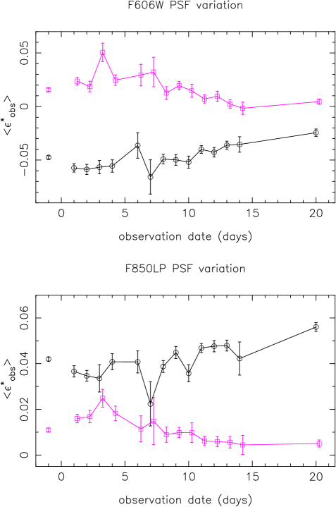
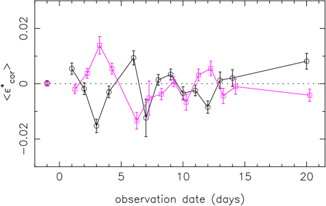
Figure 2 shows that our semi-time-dependent PSF correction reduces the average stellar ellipticity to zero and this generally holds when we measure the PSF corrected stellar ellipticity as a function of observation date, as shown in Figure 5 . There are however notable exceptions, for example ACS images taken on the third and sixth observation days, showing that the semi-time-dependent modelling is only a partial solution for time varying PSF modelling.

Figure 5: The F606W corrected stellar ellipticity parameters $\varepsilon_{1}^{{\rm cor}*}$ (circles) and $\varepsilon_{2}^{{\rm cor}*}$ (squares) averaged across the full ACS field of view as a function of observation date. The corrected stellar ellipticity averages to zero over the whole data set as shown by the isolated points on the far left of the plot. In general the PSF correction works well reducing the corrected ellipticity as a function of observation date close to zero, and significantly reducing the scatter (i.e removing the anisotropy) seen in Figure 4 (plotted on a different scale). There is however the occasional case where the stellar ellipticity is significantly different from zero showing that the semi-time-dependent modelling is only a partial solution for time varying PSF modelling. The errors plotted are the errors on the mean corrected stellar ellipticity.

To investigate the effect on the anisotropy of the PSF Figure 6 compares the difference between the stellar ellipticity predicted by the PSF models calculated for the two GEMS data sets (days 1-10 and days 11-20). To convert $\Delta p$ into a difference in stellar ellipticity we multiply by the average stellar smear polarisability $P^{\rm sm*}$ following equation (8). This comparison reveals variation in the anisotropy of the PSF at the level of, at maximum, $\Delta\varepsilon^{*}\sim 5$%. We hence conclude that the PSF time variation is not simply a change in average ellipticity but rather an instability in the PSF anisotropy across the field of view.

Creating PSF models for each ACS tile based on at maximum a few tens of stellar objects will yield systematic errors larger than the variation in the mean corrected stellar ellipticity that we see in Figure 5. Thus, the short-term PSF variation cannot be simply modelled with the method that we have used. The time dependent variation of the PSF whilst significant is at a low level and we therefore proceed with our semi-time dependent PSF model noting that short term variation in the PSF may well contribute to systematic errors (see Section 7.5).

Figure 6: The difference between stellar ellipticity calculated from PSF models for each of the two GEMS data sets with $r_{g}=5.9$ pixels. This shows that PSF variation is not a simple change in average ellipticity but also an instability in the PSF anisotropy across the field of view, varying at the maximum level of $\Delta\varepsilon^{*}=5$%.

4.2 Isotropic correction

The application of the anisotropic PSF correction to observed galaxy ellipticities, through equation (8), leaves an effectively isotropic distortion. This distortion makes objects rounder as a result of both the PSF and the Gaussian weight function used to measure the galaxy shapes, affecting smaller galaxies more strongly than the larger galaxies. To correct for this effect and convert weighted galaxy ellipticities $\varepsilon$ into unbiased shear estimators $\hat{\gamma}$, we use the pre-seeing shear polarisability tensor $P^{\gamma}$, equation (11). $P^{\gamma}$ is calculated for each galaxy from the measured galaxy smear and shear polarisability tensors, $P^{\rm sm}$ and $P^{\rm sh}$, and a term that is dependent on stellar smear and shear polarisability tensors; $\left(P^{\rm sm*}\right)_{\mu\delta}^{-1}P^{\rm sh*}_{\delta\beta}$. As the $P^{\gamma}$ correction is isotropic we can calculate this stellar term purely as a function of smoothing scale $r_{g}$, averaging over all the stellar objects that were used in the previous anisotropic PSF modelling. Note that we calculate a different value for each data set as the PSF variation we see may well be related to camera focus which will effect the $P^{\gamma}$ correction as well as the anisotropic PSF correction. $P^{\gamma}$ is a very noisy quantity, especially for small galaxies, but as we expect there to be no difference in the $P^{\gamma}$ correction for the $\gamma_{1}$ and $\gamma_{2}$ shear components, we can reduce this noise somewhat by treating $P^{\gamma}$ as a scalar equal to half its trace (note that the off diagonal terms of $P^{\gamma}$ are typically very small).

In an effort to reduce the noise on $P^{\gamma}$ still further, $P^{\gamma}$ is often fit as a function of $r_{g}$ (Hoekstra et al., 1998; Bacon et al., 2003; Brown et al., 2003; Massey et al., 2004). With space-based data this fitting method produces a bias as $P^{\gamma}$ is a strong function of galaxy ellipticity where the dependence can be demonstrated by considering that in the case of a galaxy observed in the absence of PSF smearing and shearing, $P^{\gamma}$ reduces to $P^{\gamma}=2(1-e^{2})$, where $e$ is the unweighted galaxy ellipticity. $\gamma=\varepsilon/P^{\gamma}$ is very sensitive to small errors in a functional fit of $P^{\gamma}(r_{g},\varepsilon)$ and we therefore do not use any form of fitting to $P^{\gamma}$. Although this decreases the signal-to-noise of the shear measurement, it avoids any form of shear calibration bias which would not be identified with an E/B mode decomposition as discussed in Sections 7.2.2 and 7.4.

4.3 Catalogue selection criteria

For our final PSF corrected shear catalogue we select galaxies with size $r_{g}>2.4$ pixels, galaxy shear $|\gamma|<1$, magnitude $21<{\rm m}_{606}<27$, and ${\rm SNR}>15$. We remove galaxies from the catalogue with neighbouring objects closer than $20$ pixels ($0.6$ arcsec) to reduce noise in the ellipticity measurement from overlapping isophotes. These selection criteria yield 47373 galaxies in the F606W images, a number density of $\sim 60$ galaxies per square arcminute, and 23860 galaxies in the F850LP images and a number density of $\sim 30$ galaxies per square arcminute. Note $\sim 15\%$ of our F606W sources have photometric redshift estimates from COMBO-17. We find no significant correlations of the galaxy shear with chip position, galaxy size, magnitude or SNR.

To analyse the full GEMS mosaic we rotate the shear measurements from each ACS tile into a common reference frame by

$$\left(\begin{array}[]{c}\gamma_{1}^{\rm rot}\\ \gamma_{2}^{\rm rot}\end{array}\right)=\left(\begin{array}[]{cc}\cos 2\phi&\sin 2\phi\\ -\sin 2\phi&\cos 2\phi\end{array}\right)\left(\begin{array}[]{c}\gamma_{1}\\ \gamma_{2}\end{array}\right),$$ (14)

where $\phi$ is defined to be the angle between the $x$ axis of each ACS tile and a line of constant declination.

5 Comparison of F606W and F850LP data

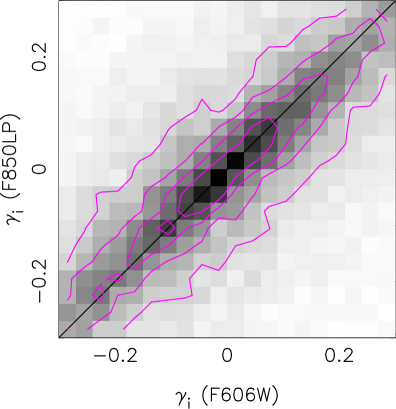
As the F850LP data is significantly shallower than the F606W data we omit it from our cosmic shear analysis, but it is interesting to use the galaxies detected in both F606W and F850LP as a consistency check to test if our method is sensitive to the differences in filter PSFs seen in Figure 1. Even though we expect galaxy morphology to appear differently in the F606W and F850LP images, we expect our shear estimates to remain consistent. Figure 7 shows the very good agreement between galaxy shear measured in the F606W and F850LP images where the grey-scale shows the number density of objects. This comparison shows that our method of measuring shear produces very consistent results for galaxies imaged with different PSFs and different noise properties, showing no significant calibration biases. In principle one should correct the galaxy ellipticity based on galaxy colour because of the chromatic anisotropy of the PSF, but this comparison also shows that the colour of the PSF does not significantly impact on the shear measurement.

Figure 7: Comparison of galaxy shear $\gamma_{i}$ measured in both F606W and F850LP GEMS imaging. The grey-scale shows the number density of objects which cluster at low shear values (black $=210$ galaxies, white $\rightarrow 0$ galaxies). Over-plotted are the grey-scale contours which follow the 1:1 relationship that we would wish to see between the two data sets.

6 GEMS redshift distribution

To interpret a weak lensing signal we need to know the redshift distribution of the lensed sources (see equation (2)). The deeper the survey is, the stronger the signal we expect to measure. We estimate the source redshift distribution of GEMS based on photometric redshifts from the CDFS COMBO-17 survey (Wolf et al., 2004) and spectroscopic redshifts from the CDFS VVDS survey (Le Fèvre et al., 2004), by assuming that a magnitude dependent redshift distribution can be parameterised as

$$n(z,{\rm mag})\propto z^{2}\exp\left[-\left(\frac{z}{z_{0}({\rm mag})}\right)^{1.5}\right]$$ (15)

where $z_{0}$ is calculated from the median redshift $z_{m}$ with $z_{0}=z_{m}/1.412$ (Baugh & Efstathiou, 1994). We calculate $z_{m}({\rm mag})$ for each survey in magnitude bins of width 0.5 magnitude, out to the limiting magnitude of each survey VVDS, ${\rm I}_{\rm AB}<24$; COMBO-17, ${\rm R}_{\rm Vega}<24$. These estimates are taken as lower limits for the true median redshift, as both surveys suffer from redshift incompleteness at faint magnitudes. To calculate upper limits for the true median redshift we follow Brown et al. (2003) assuming those galaxies without an assigned redshift are most likely to be at a higher redshift. We place the percentage of galaxies without redshift measurements at $z=\infty$ and re-calculate $z_{m}({\rm mag})$, taking our final median redshift estimate to be the midpoint between this upper limit and the measured lower limit. In the cases where the difference between our upper and lower limit constraints are larger than the error on the mean of the distribution $\sigma_{z}/\sqrt{N}$ the uncertainty on the median redshift is given by the upper and lower limits. For bright magnitudes where the redshift measurements are fairly complete and the number density of objects are relatively small, we place a statistical uncertainty on the median redshift given by $\sigma_{z}/\sqrt{N}$. For the COMBO-17 median redshift error we include the additional error on the photometric redshift estimate where $\delta z/(1+z)\sim 0.02$ for ${\rm R}_{\rm Vega}<22$ and $\delta z/(1+z)\sim 0.05$ for $22<{\rm R}_{\rm Vega}<24$.

Figure 8: The median galaxy redshift as a function of ${\rm m}_{606}$ magnitude based on photometric redshifts from COMBO-17 (squares) and the HDFN (triangles), and spectroscopic redshifts from VVDS (circles). Median redshift errors include uncertainty in redshift completeness which dominates the COMBO-17 and VVDS results at faint magnitudes, and statistical uncertainty which dominates in the smaller galaxy samples at bright magnitudes. For the photometric redshifts we also include the average redshift error, added in quadrature. Magnitude errors show the uncertainty in the mean ${\rm m}_{606}$ magnitude in each magnitude bin selected in ${\rm I}_{\rm AB}$ (VVDS), ${\rm R}_{\rm Vega}$ (COMBO-17) and ${\rm m}_{606}$ (HDFN). Over-plotted is the best linear fit to the COMBO-17 and VVDS data. The HDFN data is shown at faint magnitudes to justify our extrapolation to faint magnitudes of the COMBO-17/VVDS linear fit.

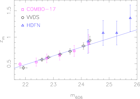
To convert the $z_{m}({\rm mag})$ from the different surveys to $z_{m}({\rm m}_{606})$ we match the COMBO-17 and VVDS sources to the CDFS 5 epoch GOODS ${\rm m}_{606}$ catalogue (Giavalisco et al., 2004). Note that matching the comparatively shallow redshift catalogues with deep 5 epoch GOODS data ensures that we are not subject to incompleteness in the ${\rm m}_{606}$ data. We then calculate the mean ${\rm m}_{606}$ in each ${\rm I}_{\rm AB}$ and ${\rm R}_{\rm Vega}$ magnitude bin, assigning an uncertainty in the ${\rm m}_{606}$ magnitude of each bin given by $\sigma_{606}/\sqrt{N}$. Figure 8 shows the combined results from both surveys which are in very good agreement, and the best linear fit;

$$z_{m}=-3.132+0.164\,{\rm m}_{606}\,\,\,\,\,\,\,(21.8<{\rm m}_{606}<24.4).$$ (16)

To estimate the median redshift of our galaxy sample fainter than ${\rm m}_{606}=24.4$ we extrapolate the above relationship. This is justified by the $z_{m}:{\rm m}_{606}$ relationship measured in the Hubble Deep Field North (HDFN) (Lanzetta et al., 1996; Fernández-Soto et al., 1999) shown (triangles) in Figure 8, where the median redshift error combines the photometric redshift error $\delta z/(1+z)\sim 0.1$ (Fernández-Soto et al., 1999) and the statistical uncertainty in each bin. Note that only the ${\rm m}_{606}>24$ points are shown for clarity, but there is also good agreement between COMBO-17, VVDS and HDFN at brighter magnitudes

We estimate the redshift distribution for GEMS $\phi(z)$ through

$$\phi(z)=\sum_{i=1}^{M}N(i)n(z,{\rm m}_{606}(i))/\sum_{i=1}^{M}N(i)$$ (17)

where we bin the GEMS sources into $i=1,M$ magnitude slices of mean magnitude ${\rm m}_{606}(i)$, where each bin contains $N(i)$ galaxies. $n(z,{\rm m}_{606}(i))$ is calculated through equation (15) with $z_{0}({\rm m}_{606})=z_{m}({\rm m}_{606})/1.412$ as estimated from equation (16). The calculated $\phi(z)$ is very similar to a magnitude independent $n(z)$ equation (15), with $z_{m}=1.0$ and as such, for simplicity when deriving the weak lensing theoretical models in the following analyses, we will use a magnitude independent $n(z)$ with $z_{m}=1.0\pm 0.1$, where the error given derives from the accuracy of the $z_{m}({\rm m}_{606})$ fit, shown in Figure 8.

7 Analysis: 2-point statistics

In this section we use GEMS F606W data to measure the shear correlation function, the shear variance statistic and the shear power spectrum performing several diagnostic tests for systematic errors. We also determine an additional sampling error in order to account for the fact that GEMS images only one field.

7.1 Jackknife Method

In the analysis that follows we will often make use of the jackknife statistical method (see for example Wall & Jenkins 2003) to obtain correlation functions with a robust estimate of the covariance matrix. The algorithm is quite simple, if a little time consuming. We are interested in the two-point correlation function which we first calculate from the whole survey and write as a data vector $C=C(\theta_{1},\theta_{2},......)$. We then divide our sample into $N$ separate sub-regions on the sky of approximately equal area and calculate the correlation function $C_{l}=C_{l}(\theta_{1},\theta_{2},......)$, $l=1..N$ times omitting one sub-region in each calculation. Note that for a traditional jackknife we would perform the measurement $N=N_{\rm galaxy}$ times removing a single galaxy each time, but this is computationally prohibited and provided $N$ is larger than the number of angular bins, this modified jackknife method is valid (Scranton et al., 2002). Defining

$$C_{l}^{*}=NC-(N-1)C_{l}\,,$$ (18)

the jackknifed estimate of the correlation function, $\hat{C}$, is then given by the average $\hat{C}=\langle C_{l}^{*}\rangle$. The jackknife estimated statistical covariance of the correlation function $C(\theta_{i})$ in angular bin $i$ and the correlation function $C(\theta_{j})$ in angular bin $j$ is given by

$$\langle\Delta C(\theta_{i})\Delta C(\theta_{j})\rangle=\frac{1}{N(N-1)}\times$$ (19)

$$\sum_{l=1}^{l=N}\left(C_{l}^{*}(\theta_{i})-\hat{C}(\theta_{i})\right)\left(C_{l}^{*}(\theta_{j})-\hat{C}(\theta_{j})\right).$$

7.2 Tests for PSF contamination

In this section we perform several diagnostic tests to determine whether residual PSF-related correlations remain after the PSF correction of Section 4. Measuring the magnitude of PSF contamination as a function of angular scale enables us to determine which angular scale shear correlations are free from sources of systematic errors and are therefore useful for cosmological parameter estimation.

7.2.1 Star-galaxy cross correlation

Bacon et al. (2003) show that residual PSF-related distortions add a component $C_{ij}^{\rm sys}$ to the measured correlation function $\langle\gamma_{i}\gamma_{j}\rangle$ where

$$C_{ij}^{\rm sys}=\frac{\langle\gamma_{i}\varepsilon_{j}^{*}\rangle\langle\gamma_{j}\varepsilon_{i}^{*}\rangle}{\langle\varepsilon_{i}^{*}\varepsilon_{j}^{*}\rangle}.$$ (20)

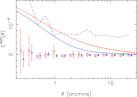
This method to test for residual PSF contamination in the data is similar to the cell averaged test described in Section 4 but in this case we look for correlations as a function of angular scale, not chip position, thereby revealing any PSF time variation effects that remain after our semi-time-dependent PSF correction has been applied. We estimate $C_{ij}^{\rm sys}$ and associated errors using the modified jackknife method detailed in Section 7.1, with $\varepsilon_{i}^{*}$ determined at $r_{g}=5.9$, the median galaxy size in the survey. We use $N=25$ sub-regions in the jackknife estimate of $M=14$ logarithmic angular bins from $\theta=0.2$ arcmin to $\theta=25$ arcmin. Figure 9 shows the resulting star-galaxy cross correlation functions $C_{tt}^{\rm sys}$ and $C_{rr}^{\rm sys}$, compared to theoretical galaxy-galaxy shear correlation functions with $\Omega_{m}=0.3$, and $\sigma_{8}=0.75$. We find that the star-galaxy cross correlation is consistent with zero indicating that the measurement of galaxy-galaxy shear correlations from the GEMS data will be free from major sources of systematics. For comparison we also measure the star-galaxy cross correlation when we have not included a correction for the distorting PSF. This reveals a correlation signal (shown dashed) that exceeds the weak cosmological signal that we wish to measure, stressing the importance for a good understanding of the PSF.

Figure 9: Star-galaxy cross correlation functions $C_{tt}^{\rm sys}$ (circles) and $C_{rr}^{\rm sys}$ (crosses) compared to theoretical galaxy-galaxy shear correlation functions $\langle\gamma_{r}\gamma_{r}\rangle_{\theta}$ (upper curve) and $\langle\gamma_{t}\gamma_{t}\rangle_{\theta}$ (lower curve) with $z_{m}=1.0$, $\Omega_{m}=0.3$, and $\sigma_{8}=0.7$. For comparison we also measure the star-galaxy cross correlation in the absence of PSF corrections, shown dashed, where for clarity we plot $\frac{1}{2}(C_{tt}^{\rm sys}+C_{rr}^{\rm sys})$.

7.2.2 E/B mode decomposition of shear correlations

An alternative diagnostic to determine the level of systematic errors is to decompose the shear correlation function into ‘E-modes’ and ‘B-modes’ (Crittenden et al., 2002). Weak gravitational lensing produces gradient curl-free distortions (E-mode), and contributes only to the curl distortions (B-mode) at small angular scales, $\theta<1$ arcmin, due to source redshift clustering (Schneider et al., 2002). A significant detection of a B-type signal in weak lensing surveys is therefore an indication that ellipticity correlations exist from residual systematics within the data and/or from intrinsic galaxy alignments (see Heymans et al. (2004) for a discussion of the latter).

Defining the sum and difference of the tangential and rotated correlation functions,

$$\xi_{\pm}(\theta)=\langle\gamma_{t}\gamma_{t}\rangle_{\theta}\pm\langle\gamma_{r}\gamma_{r}\rangle_{\theta},$$ (21)

Crittenden et al. (2002) show that the shear correlation functions can be decomposed into the following E- and B-type correlators,

$$\xi^{E}(\theta)=\frac{\xi_{+}(\theta)+\xi^{\prime}(\theta)}{2}\ \ \ \ \ \ \xi^{B}(\theta)=\frac{\xi_{+}(\theta)-\xi^{\prime}(\theta)}{2}$$ (22)

where

$$\xi^{\prime}(\theta)=\xi_{-}(\theta)+4\int_{\theta}^{\infty}\frac{d\vartheta}{\vartheta}\xi_{-}(\vartheta)-12\theta^{2}\int_{\theta}^{\infty}\frac{d\vartheta}{\vartheta^{3}}\xi_{-}(\vartheta).$$ (23)

Our data extends at maximum to $\theta=28$ arcmin necessitating the use of a fiducial cosmological model to complete the integral. This prevents cosmological parameter estimation directly from the E-modes, but as the variation in the sum of the model dependent part of the integral is small $\sim 10^{-5}$, this method is still a valid diagnostic test for residual systematics within the data. Note that the mass aperture statistic E/B decomposition (Schneider et al., 1998) does not suffer from this limitation as the integral over the shear correlation function spans from $0\rightarrow 2\theta$. This integral range does however introduce its own problems (see Massey et al. 2004 for a discussion) and limits the analysis to small scale power (Van Waerbeke et al., 2005). We therefore choose to use the E and B type correlators purely to test for B-type systematic errors within our data, although see Van Waerbeke et al. (2005) for a method that uses the mass aperture statistic to calibrate $\xi^{E}(\theta)$ for cosmological parameter estimation.

Figure 10: E/B mode decomposition of the shear correlation function measured from the GEMS observations. The upper panel shows $\xi^{\rm bin}_{E}$ and the fiducial $\Lambda{\rm CDM}$ theoretical $\xi^{E}(\theta)$ model where $\sigma_{8}=0.7$ and the median source redshift $z_{m}=1.0$. The lower panel shows $\xi^{\rm bin}_{B}$ that is consistent with zero on all angular scales and can be compared to the theoretical model $\xi^{E}(\theta)$ shown dotted. Using a different fiducial $\Lambda{\rm CDM}$ cosmological model to calculate $\xi^{\rm bin}$ has a small effect (at the level of $10^{-5}$) which can be seen from the dotted curves where we have assumed $\sigma_{8}=0.6$ (lower curve E-mode, upper curve B-mode) and $\sigma_{8}=1.0$ (upper curve E-mode, lower curve B-mode)

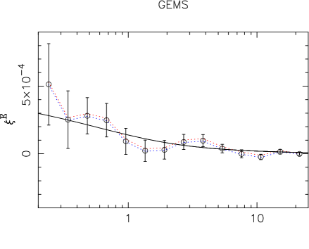
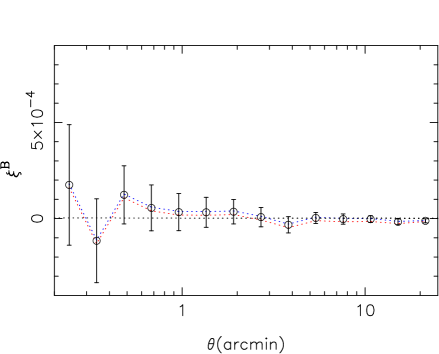
Following Pen et al. (2002) we define the $2n$ element vector $\xi_{i}=(\xi_{+}(\theta),\xi_{-}(\theta))$ which we compute from GEMS, binning the data finely into $n=2000$ intervals of $0.9$ arcsec (equivalent to a separation of $\sim 30$ ACS pixels). The E/B correlators are then given by a $2n$ element vector

$$\xi^{EB}_{i}=(\xi^{E}(\theta_{i}),\xi^{B}(\theta_{i}))=T_{ij}\xi_{j}$$ (24)

where $T$ is a $2n^{2}$ transformation matrix defined by equation (23). To reduce noise we re-bin $\xi^{EB}_{i}$ into $M=14$ logarithmic intervals from $\theta=0.2$ arcmin to $\theta=25.0$, represented by an $M\times 2n$ projection operator $\xi^{\rm bin}_{k}=P_{ki}\xi^{EB}_{i}$.

To calculate errors on $\xi^{\rm bin}_{k}$ we first calculate the covariance matrix of the raw correlators $L_{ij}=\langle\Delta\xi_{i}\Delta\xi_{j}\rangle$ using the jackknife method detailed in Section 7.1. We find, in contrast to Pen et al. (2002), that our slightly wider correlation bins ($\Delta\theta=0.9$ arcsec compared to $\Delta\theta=0.6$ arcsec) are correlated. Note that the modified jackknife method in principle requires $N>n$ sub-regions to calculate $L_{ij}$, but as we re-bin $L_{ij}$ into $M=14$ broader angular scales to estimate the final errors on $\xi^{\rm bin}$ our jackknife method, which is computationally time limited to $N=100$, is still valid. The binned covariance matrix of the E/B correlators is given by (Pen et al., 2002),

$$L^{\rm bin}_{lm}=P_{li}T_{ij}L_{jk}T_{ko}P_{om},$$ (25)

where the errors on $\xi^{\rm bin}_{k}$ are given by $\sqrt{L^{\rm bin}_{kk}}$.

We investigate E- and B-mode correlations in the GEMS and GOODS data separately with the measurement from the GEMS data shown in Figure 10. For this E/B mode decomposition we have used a fiducial $\Lambda{\rm CDM}$ cosmological model to complete the integral of equation (23) with $\sigma_{8}=0.7$ and with a median source redshift for our galaxies of $z_{m}=1.0$. Using a different fiducial $\Lambda{\rm CDM}$ cosmological model has a small effect (at the level of $10^{-5}$) which can be seen from the dotted curves in Figure 10 where we have assumed $\sigma_{8}=0.6$ and $\sigma_{8}=1.0$. We find that the E-modes are in good agreement with the fiducial cosmological model and that the B-modes for GEMS are consistent with zero on all scales $\theta>0.2$ arcmin. Whilst finding this result very encouraging we note that our B-modes measured at small angular scales are very strongly correlated and noisy such that in the worse-case scenario, represented by the upper end of the error bars shown, the B-modes exceed the signal that we wish to measure. This motivates our desicion to conservatively limit our shear correlation function analysis to angular scales $\theta>0.65$ arcmins within the GEMS data where we can be confident that the signal we measure is cosmological and not systematic.

The PSF model for the GOODS data is determined from approximately half the number of stars which were used to determine the two semi-time-dependent GEMS PSF models, as GOODS spans approximately one quarter of the area of the GEMS observations. We would therefore expect to find a poorer PSF correction with the GOODS data which is seen with the presence of non-zero B-modes at angular scales $\theta<1$ arcmin. We therefore only include GOODS data in our shear correlation function analysis for angular scales $\theta>1$ arcmin.

7.3 The shear correlation function

Having shown in the previous section that we are not contaminated by significant non-lensing correlations, we can now measure the weak lensing shear correlation function $\langle\gamma(\mbox{\boldmath{$\theta$}})\gamma(\mbox{\boldmath{$\theta$}}+\Delta\theta)\rangle$. To obtain results that are independent of the initial frame of reference we measure the tangential and rotated shear correlation functions, equation (3) and equation (4) respectively. These can be estimated from the data by

$$E[\gamma_{{}_{r}^{t}}\gamma_{{}_{r}^{t}}]_{\theta}=\frac{1}{\rm Npairs}\sum_{\rm pairs}\gamma_{{}_{r}^{t}}({\bf x})\,\gamma_{{}_{r}^{t}}({\bf x}+\mbox{\boldmath{$\theta$}}),$$ (26)

where the tangential shear $\gamma_{t}$ and rotated shear $\gamma_{r}$ are given by equation (14). $\gamma_{t}=\gamma_{1}^{\rm rot}$ and $\gamma_{r}=\gamma_{2}^{\rm rot}$ where the rotation angle $\phi$ is now defined to be the angle between the $x$ axis and the line joining each galaxy pair. Note this rotation follows the initial rotation that sets the full GEMS shear catalogue into the same reference frame. We also calculate the cross-correlation function $E[\gamma_{t}\gamma_{r}]_{\theta}$, which the parity invariance of weak lensing predicts to be zero.

Figure 11: Shear correlation functions $E[\gamma_{t}\gamma_{t}]_{\theta}$ (upper panel) and $E[\gamma_{r}\gamma_{r}]_{\theta}$ (lower panel) estimated from the GEMS data using a modified jackknife technique. The GOODS section of the GEMS survey is only included in measurements of $E[\gamma\gamma]_{\theta}$ for $\theta>1.0$ arcmin so as not to include the non-lensing B-mode systematics seen in the GOODS data at smaller angular scales. Over-plotted are theoretical $\Lambda CDM$ models $\langle\gamma_{t}\gamma_{t}\rangle_{\theta}$ (upper panel) and $\langle\gamma_{r}\gamma_{r}\rangle_{\theta}$ (lower panel) with $\sigma_{8}=0.6$ (dashed lower), $\sigma_{8}=0.7$ (solid) and $\sigma_{8}=1.0$ (dashed upper).

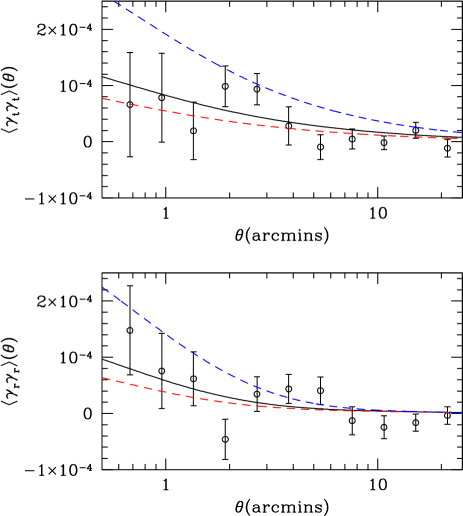
We calculate the shear correlations using the modified jackknife method detailed in Section 7.1. We use $N=25$ sub-regions in the jackknife estimate of $M=11$ logarithmic angular bins from $\theta=0.65$ arcmin to $\theta=25$ arcmin and we include data from the GOODS area only for angular scales $\theta>1$ arcmin. This ensures that the shear correlation measurement at small angular scales $\theta<1$ arcmin is not contaminated by the small-scale non-lensing distortions found in the GOODS data. We show the resulting jackknife estimates for the tangential and rotated shear correlation functions in Figure 11. The theoretical $\Lambda CDM$ models over-plotted are calculated from equation (3) and equation (4) with a median galaxy redshift $z_{m}=1.0$ and $\sigma_{8}=(0.6,0.7,1.0)$. Note that we find the cross-correlation $E[\gamma_{t}\gamma_{r}]_{\theta}$ to be consistent with zero on all scales, as expected, supporting our findings that we are not contaminated by significant non-lensing distortions.

7.3.1 Sampling variance

The GEMS mosaic samples only one area of sky and as such our results are subject to additional sampling variance errors. To address this issue we have created 100, $28\times 28$ arcmin, Gaussian realisations of a shear power spectrum calculated for a $\sigma_{8}=0.75$, $\Lambda$CDM cosmology for sources with $z_{m}=1$. We measure the shear correlation function from each realisation, populating the shear field with 60 circular galaxies per square arcmin. The variance we measure between the results from each realisation then provides us with an estimate of the sampling variance. We calculate the sampling covariance matrix from the 100 independent realisations and add this to the jackknifed covariance matrix measured from the GEMS data, slightly overestimating the sampling variance error on small scales. The reader should note that this method is somewhat cosmology dependent but it is sufficient to estimate the amplitude of sampling variance for our cosmological parameter constraints in section 8. Future work will investigate the impact of non-Gaussianity on our sampling variance estimation using the cosmological ray-tracing N-body simulations of White (2005).

7.4 The shear variance statistic

Space-based lensing surveys to date and early ground-based lensing results focused on the shear variance statistic, equation (5), to analyse the data. This statistic produces the highest signal-to-noise measurement of weak lensing shear and can be estimated from the data by splitting the sample into N circular cells of radius $\theta$ and calculating the shear variance in excess of noise (see Brown et al. 2003 for a minimum variance estimator). As discussed in Section 7.2.2 measuring the B-mode of the shear correlation function allows one to select angular scales above which one can be confident that the presence of non-lensing distortions are insignificant. Very small scale systematic distortions are poorly understood and are sucessfully ignored by the shear correlation statistic. For the shear variance statistic however, small scale non-lensing distortions are included in the measurement at all angular scales biasing the shear variance statistic.

To assess the impact of our residual small scale non-lensing distortions on the shear variance statistic we can, in a similar fashion to Section 7.2.2, decompose the signal into its E-mode and B-mode components. Schneider et al. (2002) show that the shear variance of the E- and B-mode can be obtained in terms of the shear correlation functions $(\xi_{+},\xi_{-})$, equation (21), through

$$\langle\gamma^{2}\rangle_{\theta}^{E}=\int_{0}^{\infty}\frac{d\vartheta\,\vartheta}{2\theta^{2}}\left[\xi_{+}(\vartheta)S_{+}\left(\frac{\vartheta}{\theta}\right)+\xi_{-}(\vartheta)S_{-}\left(\frac{\vartheta}{\theta}\right)\right],$$ (27)

$$\langle\gamma^{2}\rangle_{\theta}^{B}=\int_{0}^{\infty}\frac{d\vartheta\,\vartheta}{2\theta^{2}}\left[\xi_{+}(\vartheta)S_{+}\left(\frac{\vartheta}{\theta}\right)-\xi_{-}(\vartheta)S_{-}\left(\frac{\vartheta}{\theta}\right)\right],$$ (28)

where $S_{+}$ and $S_{-}$ are given in equation (39) and equation (42) of Schneider et al. (2002). Note that $S_{-}$ does not cut off at finite separation and as such one needs to include a fiducial cosmological model to complete the integral, as in Section 7.2.2. We calculate $\langle\gamma^{2}\rangle_{\theta}^{E}$ and $\langle\gamma^{2}\rangle_{\theta}^{B}$ following the method of Pen et al. (2002), detailed in Section 7.2.2, where the transformation matrix $T$ of equation (24) is now defined by equation (27) and equation (28).

Figure 12: E/B mode decomposition of the shear variance. The upper panel shows $\langle\gamma^{2}\rangle_{\theta}^{E}$ and the fiducial $\Lambda{\rm CDM}$ theoretical $\langle\gamma^{2}\rangle$ model (solid) where $\sigma_{8}=0.7$ and the median source redshift $z_{m}=1.0$. The lower panel shows $\langle\gamma^{2}\rangle_{\theta}^{B}$ that is consistent with zero on angular scales $\theta>1.5$ arcmin. Using a different fiducial $\Lambda{\rm CDM}$ cosmological model to calculate $\langle\gamma^{2}\rangle_{\theta}^{EB}$ has a small effect (at the level of $3\times 10^{-5}$) which can be seen from the dotted curves where we have assumed $\sigma_{8}=0.6$ (lower curve E-mode, upper curve B-mode) and $\sigma_{8}=1.0$ (upper curve E-mode, lower curve B-mode). The significant non-lensing B-modes at $\theta<1.5$ arcmin indicate residual small scale systematics that, with the shear variance statistic, are included at all angular scales. These non-lensing distortions also contribute to the measured E-mode making the signal appear to favour a high value for $\sigma_{8}$ (upper panel: $\Lambda{\rm CDM}$ $\sigma_{8}=1.0$ theoretical model over-plotted dot-dashed).

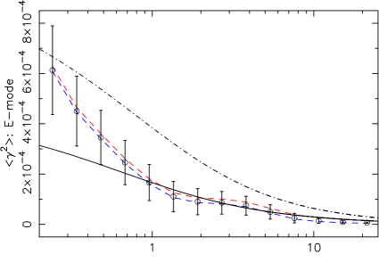
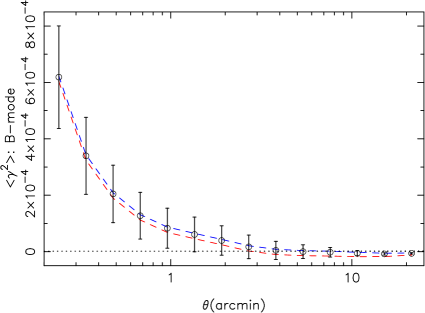
Figure 12 shows the result of our E/B mode decomposition of the shear variance statistic revealing significant B-modes on scales $\theta<1.5$ arcmin. Replacing the small scale $\xi_{+}$ and $\xi_{-}$ measurements ($\theta<0.2$ arcmin) with a theoretical model, we find B-modes consistent with zero on all scales. The B-modes shown in Figure 12 therefore result from very small scale strong non-lensing distortions that bias the shear variance statistic even at larger angular scales. Non-lensing distortions are likely to contribute equally to the measured E-mode making the signal appear to favour a higher value for $\sigma_{8}$, when compared to the large scale B-mode free shear variance measurements. These large angular scales have previously been unmeasureable from space-based data. This demonstrates that in order to obtain reliable cosmological parameter constraints it is vital to perform an E/B mode decomposition of the statistic that will be used to constrain cosmology. We will not use the shear variance statistic to constrain cosmological parameters, even on B-mode free scales, preferring the shear correlation function statistic in Section 7.3 and the shear power spectrum that we determine in the following section.

7.5 Shear power spectrum

In addition to the shear correlation function and shear variance statistic of the previous sections, we also quantify the two-point statistics of the shear field by directly measuring its power spectrum, $P_{\kappa}$, equation (1). Power spectrum estimation from cosmological data sets is a well-studied problem in the context of measuring the statistical properties of the CMB (see Efstathiou 2004 for an overview) and the methods developed in this field are completely applicable to measuring power spectra from weak lensing data sets. Here, we use a maximum likelihood estimator (see for example Bond et al. 1998) to reconstruct the power spectrum of the shear field observed in the GEMS data. Our approach is based on the prescription of Hu & White (2001) who proposed reconstructing the three power spectra, $P^{\kappa\kappa}$, $P^{\beta\beta}$ and $P^{\kappa\beta}$ as a series of step-wise ‘band-powers’ where the quantity $\ell(\ell+1)P^{ij}/2\pi$ is approximated as a constant within each band. $P^{\beta\beta}$ is the power spectrum of the B-modes while $P^{\kappa\beta}$ is the cross power-spectrum between the E- and B-modes. The maximum likelihood method automatically accounts for irregular survey geometries, pixelization effects and produces error estimates, via the Fisher Information matrix (see for example Tegmark et al. 1997), which include sampling variance and shot noise. Hu & White (2001) have tested the maximum likelihood estimator on both Gaussian and N-body simulations, while Brown et al. (2003) have tested it on Gaussian simulations on scales similar to the GEMS data and have applied the estimator to the COMBO-17 weak lensing data set.

The maximum-likelihood decomposition only necessitates the use of a fiducial cosmological model to estimate the significance of the result. This is in comparison to the E/B correlators of Section 7.2.2 and the E/B shear variance measurements of Section 7.4 where a fiducial cosmological model is needed to complete integrals over the infinite correlation function thereby invalidating their sole use for cosmological parameter estimation.

To apply the estimator to the GEMS data, we bin the galaxy shear distribution into $30\times 30$ equal-size pixels of $\sim 1$ square arcmin. Writing this pixelised shear distribution as a vector, ${\bf d}$, we then maximise the likelihood function,

$$-2\ln L({\bf C}|{\bf d})={\bf d}^{t}{\bf C}^{-1}{\bf d}+{\rm Tr}\,[\ln{\bf C}],$$ (29)

using a Newton-Raphson scheme, as a function of the band-powers of the three power spectra, $P^{\kappa\kappa}$, $P^{\beta\beta}$ and $P^{\kappa\beta}$. Here, ${\bf C}$ is the data covariance matrix which is the sum of the cosmological signal (equation (21) of Brown et al. (2003)) and a noise term,

$${\bf N}=\frac{\gamma_{\rm rms}}{N_{\rm pix}}\,\,{\bf I},$$ (30)

where $\gamma_{\rm rms}$ and $N_{\rm pix}$ are the root mean square shear and occupation number within each pixel respectively. The errors and covariance of our final band-powers are approximated as the inverse Fisher matrix, which is an excellent approximation provided that the likelihood function is sufficiently Gaussian in the band-powers.

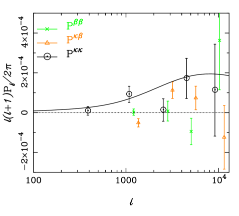
Figure 13 shows the results of applying the maximum likelihood estimator to the GEMS data along with a theoretical shear power spectrum for a $\Lambda$CDM model with $\Omega_{m}=0.3$ and $\sigma_{8}=0.8$ with which we find reasonable agreement. The measurements of the B-mode spectrum are mostly consistent with zero although there is a significant detection of E-B cross-correlations on medium scales. We suspect that these come from the time-variation of the PSF that we have only partially accounted for with our semi-time dependent PSF modelling. Our PSF models are designed to decrease the average stellar ellipticity to zero and therefore when averaging over the whole survey, as in the measurement of the shear correlation function, the residual PSF contamination is zero, as can be seen in Figure 9. For the shear power spectrum measurement however, where the field is decomposed into its Fourier components, the time-dependent PSF contamination can be identified. Note that from the covariance of the $P^{\kappa\kappa}$ measurements we find that our band-power measurements are almost independent of one another, apart from the slight anti-correlation of neighbouring bands which is a natural consequence of the maximum likelihood estimator.

Figure 13: The cosmic shear power spectra from GEMS. Plotted on a linear-log scale are $P^{\kappa\kappa}$ (circles), $P^{\beta\beta}$ (crosses) and $P^{\kappa\beta}$ (triangles) in five band-averaged band-powers as a function of multipole, $\ell$. The errors bars are estimated from the Fisher matrix and the $P^{\beta\beta}$ and $P^{\kappa\beta}$ have been slightly horizontally displaced for clarity. The solid curve is the shear power spectrum estimated for a $\sigma_{8}=0.8$ normalised $\Lambda{\rm CDM}$ model.

8 Cosmological parameter estimation

Having measured the 2-point statistics of the shear field within GEMS, we can now compare these measurements with theoretical predictions in order to place joint constraints on the matter density of the Universe $\Omega_{m}$ and the normalisation of the matter power spectrum $\sigma_{8}$. We do this using both our correlation function measurements from Section 7.3 and the power spectrum estimates from Section 7.5. We use equation (1) to calculate our theoretical shear power spectra and equation (3) and equation (4) to calculate our theoretical correlation functions for a variety of cosmological models. For these calculations we have used the transfer function of Eisenstein & Hu (1999) for the dark matter power spectrum with an initial power spectrum slope of $n=1$. To produce the non-linear power spectrum from this, we use the fitting formulae of Smith et al. (2003) and we fix $\Omega_{m}+\Omega_{\Lambda}=1$. We also use the form of equation (15) for the input redshift distribution of source galaxies. We consider models in the following regions of parameter space: $0.3\leq\sigma_{8}\leq 1.5$ ; $0.1\leq\Omega_{m}\leq 1.0$ ; $64\leq H_{0}\leq 80\,{\rm kms^{-1}Mpc^{-1}}$ and $0.9\leq z_{m}\leq 1.1$.

Figure 14: The likelihood surface of $\sigma_{8}$ and $\Omega_{m}$ from GEMS as calculated using the shear correlation function (dark contour) and using the shear power spectrum (light contours). We plot the $1\sigma$ and $2\sigma$ confidence regions for the shear power spectrum, and, for clarity, the $1\sigma$ confidence regions for the shear correlation function

Writing our correlation function measurements as a data vector,

$${\bf d}=\{C_{1}(\theta_{1}),...,C_{1}(\theta_{n}),C_{2}(\theta_{1}),...,C_{2}(\theta_{n})\},$$ (31)

for each theoretical model, we calculate

$$\chi^{2}=\left[{\bf d}-{\bf x}\right]^{T}{\bf V}^{-1}\left[{\bf d}-{\bf x}\right],$$ (32)

where ${\bf x}={\bf x}(\sigma_{8},\Omega_{m},H_{0},z_{m})$ are the theoretical correlation functions ordered in a similar manner to our data vector. ${\bf V}=\langle{\bf dd}^{T}\rangle$ is the sum of the covariance matrix of our correlation function measurements as estimated from the data using equation (19) and a sampling covariance matrix as detailed in section 7.3.1. The fitting of the power spectrum measurements is done in a similar fashion where ${\bf V}$, the covariance matrix of the band-power measurements, comes from a Fisher error analysis that automatically includes sampling variance. After calculating $\chi^{2}$ values for each of our theoretical models, we marginalise over the Hubble constant, $H_{0}$ with a prior set by the $1^{\rm st}$ year WMAP results ($H_{0}=72\pm 5$ km s^-1 Mpc^-1; Spergel et al. (2003)). We also marginalise over the median redshift of the source galaxies, $z_{m}$ using $z_{m}=1.0\pm 0.1$ as estimated in Section 6.

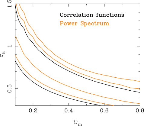
The resulting constraints in the $\sigma_{8}-\Omega_{m}$ plane for both the shear correlation function and shear power spectrum estimators are shown in Figure 14. We find good agreement between the constraints obtained using the two different measures: for the correlation function measurements, we find

$$\sigma_{8}(\Omega_{m}/0.3)^{0.65}=0.68\pm 0.13$$ (33)

while using the power spectrum analysis, we find a slightly higher value of

$$\sigma_{8}(\Omega_{m}/0.3)^{0.65}=0.72\pm 0.11.$$ (34)

9 Conclusion

In this paper we have presented the detection of weak gravitational lensing by large-scale structure in the GEMS survey, demonstrating that our shear correlation signal is uncontaminated by significant non-lensing shear distortions. GEMS, imaged by the ACS on HST, spanning $795$ square arcmin, is the largest contiguous space-based mosaic that has undergone a cosmic shear analysis to date. This has enabled us to measure cosmic shear over a large dynamic range of angular scales; from the small scales ($\theta=0.65$ arcmin) that are difficult to probe with ground-based surveys, up to the large scales ($\theta=21.0$ arcmin) that were previously inaccessible to space-based surveys. Our careful analysis, where we have considered forms of selection bias, centroid bias and calibration bias, geometric shear distortions and PSF contamination, has yielded an unbiased measurement of the shear correlation function uncontaminated by non-lensing ‘B-mode’ distortions. This has allowed us to set joint constraints uncontaminated by major sources of systematic errors on the matter density of the Universe $\Omega_{m}$ and the normalisation of the matter power spectrum $\sigma_{8}$ finding $\sigma_{8}=0.73\pm 0.13$ for WMAP constrained $\Omega_{m}=0.27$ (Spergel et al., 2003). It is interesting to note that the GEMS cosmological parameter constraints are very similar to those from the COMBO-17 survey (Brown et al., 2003; Heymans et al., 2004), a deep multi-colour survey which spans $\sim 4$ times the area of GEMS. This results from the higher number density of resolved galaxies in space-based data and the higher signal-to-noise measurements of galaxy shear which are achievable with higher resolution data (Brown et al. in prep).

We have presented a thorough discussion on the anisotropic ACS PSF that, for the first time with a space-based weak lensing analysis, we have been able to characterise directly from our data without having to assume long-term PSF stability. Long-term PSF stability has been tested with the GEMS data and shown to be true for the ACS only above the $\sim 5\%$ level. With previous space-based analyses it has often been assumed that temporal changes in the mean PSF pattern can be accommodated by a low order correction. Percent level accuracy in the ACS PSF correction would however be difficult to achieve with this assumption as this work has shown that the both the PSF strength and pattern exhibits temporal variation. We have identified PSF temporal variation on the level of a few percent finding consistent behaviour between the F850LP imaging and F606W imaging, even though the F850LP PSF is quite different from the F606W PSF. We have tested the success of our PSF correction by measuring the star-galaxy cross-correlation and the B-type shear correlator which were both found to be consistent with zero on angular scales $\theta>0.2$ arcmin. Our semi-time-dependent method for PSF modelling therefore adequately corrects for the varying PSF distortion when we consider weak lensing shear correlations as a function of relative galaxy position averaged over the whole GEMS mosaic. When we measure the shear power spectrum however, a statistic which is dependent on galaxy shear as a function of absolute galaxy position, we find a significant detection of E-B cross-correlations most likely revealing the impact of not producing a fully time-dependent PSF correction model. It is currently unclear where the variation in the GEMS ACS PSF arises but its presence, also seen by Jee et al. (2005) and Rhodes et. al. (in prep), suggests that future HST cosmic shear surveys should be preferentially observed in sequence to minimise the impact of PSF instabilities.

We have measured the commonly used top-hat shear variance statistic, performing an E/B mode decomposition. We find significant non-lensing B-mode distortions at angular scales $\theta<1.5$ arcmin in contrast to the E/B decomposition of the shear correlation function where the B-modes were found to be consistent with zero at angular scales $\theta>0.2$ arcmin. This shows that the top-hat shear variance statistic becomes contaminated by very small scale non-lensing distortions out to fairly high angular scales, strongly biasing the final result. Note that this effect is also seen in Van Waerbeke et al. (2005). The shear correlation function does not suffer from this contamination as the very small scale non-lensing correlations are removed from the analysis and it is therefore this statistic along with the shear power spectrum that we favour for cosmological parameter estimation. We urge future cosmic shear studies to perform E/B mode decompositions to test for non-lensing distortions and employ statistical analyses other than the easily biased top-hat shear variance statistic.

9.1 Comparison with other cosmic shear surveys

Figure 15: Comparison of the total shear correlation function $E[\gamma\gamma]_{\theta}$ as measured from GEMS along with the most up-to-date shear correlation measurements from the other groups indicated. Over-plotted are theoretical $\Lambda CDM$ models for a $z_{m}=1$ survey with $\sigma_{8}=0.7$ (lower) and $\sigma_{8}=1.0$ (upper). Note all data points and errors have been scaled to a $z_{m}=1$ survey using a $z_{m}^{2}$ redshift scaling.

Figure 16: Comparison of the top-hat shear variance $E[\gamma^{2}]_{\theta}$ as measured from GEMS along with the most up-to-date top-hat shear variance measurements from the other groups indicated. We show only the B-mode free GEMS top-hat shear variance results with $\theta\geq 1.5$ arcmin. Over-plotted are theoretical $\Lambda CDM$ models for a $z_{m}=1$ survey with $\sigma_{8}=0.7$ (lower) and $\sigma_{8}=1.0$ (upper). Note all data points and errors have been scaled to a $z_{m}=1$ survey using a $z_{m}^{1.85}$ redshift scaling.

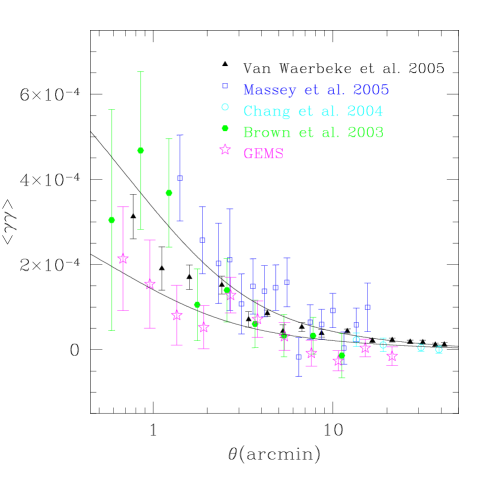
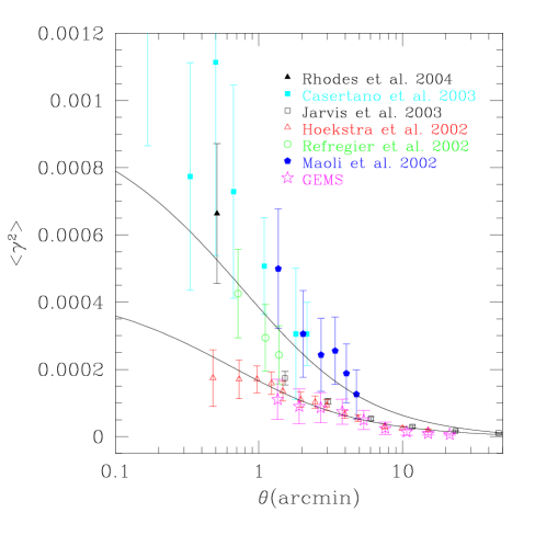
Figures 15 and 16 compare the GEMS results with the most up-to-date results from other cosmic shear surveys that have placed constraints on $\sigma_{8}$ and $\Omega_{m}$. The cosmic shear signal scales with the depth of the survey and so we have introduced a median redshift scaling of the data points and errors to bring the different results in line with a survey of median redshift $z_{m}=1.0$. For the shear correlation function (Figure 15) we scale by $z_{m}^{2}$, as suggested by the numerical simulations of Barber (2002) and for the top-hat shear variance (Figure 16) we scale by $z_{m}^{1.85}$ (Rhodes et al., 2004). We preferentially show the shear correlation function for surveys that have measured the top-hat shear variance in addition, due to our concern with the use of the top-hat shear variance statistic. We only show the B-mode free GEMS top-hat shear variance results with $\theta\geq 1.5$ arcmin. These comparisons show broad agreement between the shear correlation measurements and a poorer agreement between the top-hat shear variance measurements. As discussed in Section 7.4, the top-hat shear variance appears to be easily contaminated at large scales by small scale systematic errors and we propose that this contamination, not always quantified, is at least a partial cause of the differing results. Other possibilities are potential calibration biases arising from differences between the various shear measurement methods (compare for example Erben et al. 2001 and Bacon et al. 2001), differences in the median redshift determination and sampling variance.

The results shown in Figure 15 and Figure 16 yield measurements of $\sigma_{8}$ ranging from $\sigma_{8}\simeq 0.7$ to $\sigma_{8}\simeq 1.1$ for a value of $\Omega_{m}=0.3$. This can be compared with results from the WMAP CMB experiment (Spergel et al., 2003) that finds $\sigma_{8}=0.9\pm 0.1$ from the WMAP data alone and $\sigma_{8}=0.84\pm 0.04$ when the WMAP data is combined with other data sets. Results from cluster abundance measurements range from $\sigma_{8}=0.7$ to $\sigma_{8}=1.0$ (see Pierpaoli et al. 2003, who find $\sigma_{8}=0.77\pm 0.05$, and references therein). Our measurement is at the lower end of all these results which we may expect in light of the fact that the CDFS is a factor of two under-dense in massive galaxies (Wolf et al., 2003). If we assume that massive galaxies trace the underlying dark matter distribution, then we would expect a low measurement of $\sigma_{8}$ from this field when compared to the global $\sigma_{8}$ value. Combining GEMS data with other wide-field space-based mosaics, such as the COSMOS survey and the ACS pure parallel survey, will reduce the effects of sampling variance in order to obtain a good estimate of the Universal value of $\sigma_{8}$ from HST.

10 Acknowledgements

This work is based on observations taken with the NASA/ESA Hubble Space Telescope, which is operated by the Association of Universities for Research in Astronomy, Inc. (AURA) under NASA contract NAS5-26555. Support for the GEMS project was provided by NASA through grant number GO-9500 from the Space Telescope Science Institute, which is operated by AURA for NASA, under contract NAS5-26555. CH and HWR acknowledge financial support from GIF. MLB and CW were supported by PPARC fellowships. EFB and SFS acknowledge financial support provided through the European Community’s Human Potential Program under contract HPRN-CT-2002-00316, SISCO (EFB) and HPRN-CT-2002-00305, Euro3D RTN (SFS). SJ and DHM acknowledge support from NASA under LTSA Grant NAG5-13063(SJ) and under LTSA Grant NAG5-13102(DHM), issued through the Office of Space Science. We thank Justin Albert, Colin Cox, Richard Ellis, Yannick Mellier, John Peacock, Jason Rhodes, Tim Schrabback, Ludovic Van Waerbeke and Martin White for many useful discussions, and also the referee for his/her helpful comments.

References

- Bacon et al. (2003) Bacon D., Massey R., Refregier A., Ellis R., 2003, MNRAS, 344, 673
- Bacon et al. (2000) Bacon D., Refregier A., Ellis R., 2000, MNRAS, 318, 625
- Bacon et al. (2001) Bacon D. J., Refregier A., Clowe D., Ellis R. S., 2001, MNRAS, 325, 1065
- Barber (2002) Barber A. J., 2002, MNRAS, 335, 909
- Barden et al. (2004) Barden M., Rix H.-W., Somerville R. S., Bell E. F., Häußler B., Beckwith S. V. W., Borch A., Caldwell J. A. R., Heymans C., Jahnke K., Jogee S., McIntosh D. H., Meisenheimer K., Peng C. Y., Sanchez S. F., Wisotzki L., Wolf C., 2004, ApJ submitted, astroph/0502416
- Bartelmann & Schneider (2001) Bartelmann M., Schneider P., 2001, Physics Reports, 340, 291
- Baugh & Efstathiou (1994) Baugh C. M., Efstathiou G., 1994, MNRAS, 267, 323
- Bernstein & Jarvis (2002) Bernstein G. M., Jarvis M., 2002, AJ, 123, 583
- Bertin & Arnouts (1996) Bertin E., Arnouts S., 1996, A&AS, 117, 393
- Bond et al. (1998) Bond J. R., Jaffe A. H., Knox L., 1998, Phys. Rev. D, 57, 2117
- Brown et al. (2003) Brown M., Taylor A., Bacon D., Gray M., Dye S., Meisenheimer K., Wolf C., 2003, MNRAS, 341, 100
- Casertano et al. (2003) Casertano S., Ratnatunga K. U., Griffiths R. E., 2003, ApJL, 598, L71
- Chang et al. (2004) Chang T., Refregier A., Helfand D. J., 2004, ApJ, 617, 794
- Contaldi et al. (2003) Contaldi C., Hoekstra H., Lewis A., 2003, Phys. Rev. Lett., 90, 303
- Cox & Gilliland (2002) Cox C., Gilliland R. L., 2002, in The 2002 HST Calibration Workshop The Effect of Velocity Aberration on ACS Image Processing. pp 58–+
- Crittenden et al. (2002) Crittenden R., Natarajan R., Pen U., Theuns T., 2002, ApJ, 568, 20
- Efstathiou (2004) Efstathiou G., 2004, MNRAS, 349, 603
- Eisenstein & Hu (1999) Eisenstein D. J., Hu W., 1999, ApJ, 511, 5
- Erben et al. (2001) Erben T., Van Waerbeke L., Bertin E., Mellier Y., Schneider P., 2001, A&A, 366, 717
- Fernández-Soto et al. (1999) Fernández-Soto A., Lanzetta K. M., Yahil A., 1999, ApJ, 513, 34
- Ford et al. (2003) Ford et al. H. C., 2003, in Proceedings of the SPIE, Volume 4854, pp. 81-94 (2003). Overview of the Advanced Camera for Surveys on-orbit performance. pp 81–94
- Giavalisco et al. (2004) Giavalisco et al. M., 2004, ApJL, 600, L93
- Hämmerle et al. (2002) Hämmerle H., Miralles J.-M., Schneider P., Erben T., Fosbury R. A. E., Freudling W., Pirzkal N., Jain B., White S. D. M., 2002, A&A, 385, 743
- Hamana et al. (2003) Hamana T., Miyazaki S., Shimasaku K., Furusawa H., Doi M., Hamabe M., Imi K., Kimura M., Komiyama Y., Nakata F., Okada N., Okamura S., Ouchi M., Sekiguchi M., Yagi M., Yasuda N., 2003, ApJ, 597, 98
- Heymans et al. (2004) Heymans C., Brown M., Heavens A., Meisenheimer K., Taylor A., Wolf C., 2004, MNRAS, 347, 895
- Heymans & Heavens (2003) Heymans C., Heavens A., 2003, MNRAS, 339, 711
- Hirata & Seljak (2003) Hirata C., Seljak U., 2003, MNRAS, 343, 459
- Hoekstra et al. (1998) Hoekstra H., Franx M., Kuijken K., Squires G., 1998, ApJ, 504, 636
- Hoekstra et al. (2002) Hoekstra H., Yee H., Gladders M., 2002, ApJ, 577, 595
- Hu & White (2001) Hu W., White M., 2001, ApJ, 554, 67
- Jain & Taylor (2003) Jain B., Taylor A., 2003, Physical Review Letters, 91, 141302
- Jarvis et al. (2005) Jarvis M., Bernstein B. J. G., Dolney D., 2005, ApJ in press, astroph/0502243
- Jarvis et al. (2003) Jarvis M., Bernstein G., Jain B., Fischer P., Smith D., Tyson J., Wittman D., 2003, ApJ, 125, 1014
- Jee et al. (2005) Jee M. J., White R. L., Benítez N., Ford H. C., Blakeslee J. P., Rosati P., Demarco R., Illingworth G. D., 2005, ApJ, 618, 46
- Kaiser (2000) Kaiser N., 2000, ApJ, 537, 555
- Kaiser et al. (1995) Kaiser N., Squires G., Broadhurst T., 1995, ApJ, 449, 460
- King & Schneider (2002) King L., Schneider P., 2002, A&A, 396, 411
- Koekemoer et al. (2003) Koekemoer A. M., Fruchter A. S., Hack W. J., Hook R. N., 2003, in HST Calibration Workshop (STScI: Baltimore) Multi-drizzle. p. 337
- Krist (2000) Krist J., 2000, TinyTim User’s Guide v4. (STScI)
- Lanzetta et al. (1996) Lanzetta K. M., Yahil A., Fernández-Soto A., 1996, Nature, 381, 759
- Le Fèvre et al. (2004) Le Fèvre et al. O., 2004, A&A, 428, 1043
- Luppino & Kaiser (1997) Luppino G. A., Kaiser N., 1997, ApJ, 475, 20
- MacDonald et al. (2004) MacDonald E. C., Allen P., Dalton G., Moustakas L. A., Heymans C., Edmondson E., Blake C., Clewley L., Hammell M. C., Olding E., Miller L., Rawlings S., Wall J., Wegner G., Wolf C., 2004, MNRAS, 352, 1255
- Maoli et al. (2001) Maoli R., Van Waerbeke L., Mellier Y., Schneider P., Jain B., Bernardeau F., Erben T., 2001, A&A, 368, 766
- Massey et al. (2004) Massey R., Bacon D., Refregier A., Ellis R., 2004, MNRAS submitted, astroph/0404195
- Massey & Refregier (2004) Massey R., Refregier A., 2004, MNRAS submitted, astroph/0408445
- Massey et al. (2004) Massey R., Rhodes J., Refregier A., Albert J., Bacon D., Bernstein G., Ellis R., Jain B., McKay T., Perlmutter S., Taylor A., 2004, AJ, 127, 3089
- Meurer et al. (2003) Meurer G. R., Lindler D. J., Blakeslee J., Cox C. R., Martel A., Tran H. D., Bouwens R., Ford H. C., Clampin M., Hartig G. F., Sirianni M., De Marchi G., 2003, in Proceedings of the SPIE, Volume 4854, pp. 507-514 (2003). Calibration of geometric distortion in the ACS detectors. pp 507–514
- Miralles et al. (2005) Miralles J.-M., Erben T., Hämmerle H., Schneider P., Freudling W., Pirzkal N., Fosbury R. A. E., 2005, A&A, 432, 797
- Park et al. (2004) Park Y., Casertano S., Ferguson H. C., 2004, ApJL, 600, L159
- Pen et al. (2002) Pen U.-L., Van Waerbeke L., Mellier Y., 2002, ApJ, 567, 31
- Peng et al. (2002) Peng C. Y., Ho L. C., Impey C. D., Rix H.-W., 2002, AJ, 124, 266
- Pierpaoli et al. (2003) Pierpaoli E., Borgani S., Scott D., White M., 2003, MNRAS, 342, 163
- Refregier & Bacon (2003) Refregier A., Bacon D., 2003, MNRAS, 338, 48
- Refregier et al. (2004) Refregier A., Massey R., Rhodes J., Ellis R., Albert J., Bacon D., Bernstein G., McKay T., Perlmutter S., 2004, AJ, 127, 3102
- Refregier et al. (2002) Refregier A., Rhodes J., Groth E. J., 2002, ApJL, 572, L131
- Rhodes et al. (2004) Rhodes J., Refregier A., Collins N. R., Gardner J. P., Groth E. J., Hill R. S., 2004, ApJ, 605, 29
- Rhodes et al. (2000) Rhodes J., Refregier A., Groth E. J., 2000, ApJ, 536, 79
- Rhodes et al. (2001) Rhodes J., Refregier A., Groth E. J., 2001, ApJL, 552, L85
- Rhodes et al. (2004) Rhodes J., Refregier A., Massey R., Albert J., Bacon D., Bernstein G., Ellis R., Jain B., Kim A., Lampton M., McKay T., SNAP Collaboration 2004, Astroparticle Physics, 20, 377
- Riess (2002) Riess A., 2002, in The 2002 HST Calibration Workshop Growth of Hot Pixels and Degradation of CTE for ACS. pp 47–+
- Riess et al. (2004) Riess et al. A. G., 2004, ApJL, 600, L163
- Rix et al. (2004) Rix H.-W., Barden M., Beckwith S. V. W., Bell E. F., Borch A., Caldwell J. A. R., Häußler B., Jahnke K., Jogee S., McIntosh D. H., Meisenheimer K., Peng C. Y., Sánchez S. F., Somerville R. S., Wisotzki L., Wolf C., 2004, ApJS, 152, 163
- Schneider et al. (1998) Schneider P., Van Waerbeke L., Jain B., Kruse G., 1998, MNRAS, 296, 873
- Schneider et al. (2002) Schneider P., Van Waerbeke L., Mellier Y., 2002, A&A, 389, 741
- Scranton et al. (2002) Scranton et al. R., 2002, ApJ, 579, 48
- Smith et al. (2003) Smith R., Peacock J., Jenkins A., White S., Frenk C., Pearce F., Thomas P., Efstathiou G., Couchman. H., 2003, MNRAS, 341, 1311
- Spergel et al. (2003) Spergel D., Verde L., Peiris H., WMAP Collaboration 2003, ApJS, 148, 175
- Tegmark et al. (1997) Tegmark M., Taylor A. N., Heavens A. F., 1997, ApJ, 480, 22
- Tereno et al. (2005) Tereno I., Doré O., van Waerbeke L., Mellier Y., 2005, A&A, 429, 383
- Van Waerbeke et al. (2005) Van Waerbeke L., Mellier Y., Hoekstra H., 2005, A&A, 429, 75
- Van Waerbeke et al. (2001) Van Waerbeke L., Mellier Y., Radovich M., Bertin E., Dantel-Fort M., McCracken H., Fèvre O. L., Foucaud S., Cuillandre J., Erben T., Jain B., Schneider P., Bernardeau F., Fort B., 2001, A&A, 374, 757
- Wall & Jenkins (2003) Wall J. V., Jenkins C. R., 2003, Practical statistics for astronomers. Princeton Series in Astrophysics
- White (2005) White M., 2005, Aph in press astroph/0502003
- Wolf et al. (2004) Wolf C., Meisenheimer K., Kleinheinrich M., Borch A., Dye S., Gray M., Wisotzki L., Bell E., Rix H.-W., Hasinger A. C. G., Szokoly G., 2004, A&A, 421, 913
- Wolf et al. (2003) Wolf C., Meisenheimer K., Rix H.-W., Borch A., Dye S., Kleinheinrich M., 2003, A&A, 401, 73