A Robust Algorithm for the Pointing Refinement and Registration of Astronomical Images

Abstract

We present a generic algorithm for performing astronomical image registration and pointing refinement. The method is based on matching the positions and fluxes of available point sources in image overlap regions. This information is used to compute a set of image offset corrections by globally minimizing a weighted sum of all matched point-source positional differences in a pre-specified reference image frame. A fast linear sparse matrix solver is used for the minimization. From these corrections, the pointings and orientations of images can be refined in either a relative sense where pointings become fixed (registered) relative to a single input image, or, in an absolute sense (in the ICRS) if absolute point source information is known. The latter provides absolute pointing refinement to an accuracy depending on the robustness of point source extractions, match statistics, and accuracy of the astrometric catalog used. The software is currently used in the Spitzer image processing pipelines, although it is adaptable to any astronomical imaging system which uses the FITS image format and WCS pointing standard.

We test the algorithm using Monte Carlo simulations and compare them to image data acquired with the Infrared Array Camera (IRAC) on board the Spitzer Space Telescope. We find that dispersions in matched source separations after refinement are entirely consistent with centroiding errors in source extractions, implying that systematic uncertainties due to inaccurately calibrated distortions are negligible. For these data, we predict refinements to better than $\sim 70$ and $\sim 280$ mas ($2\sigma$ radial) for the IRAC $3.6$ and $8\micron$ bands respectively. These bands bracket two extremes in available source matches and, for the data under study, correspond to an average of about 55 and 8 matches per image in these two bands respectively.

1 Introduction

The need to register or co-align images in astronomy to an accuracy better than the Nyquist sampling density of a detector’s point response function is pivotal if one wants to maximize the resolution and signal-to-noise attainable in a mosaic of co-added images. The absolute accuracy is inhibited by instabilities in telescope pointing control, tracking sensors, and how these behave in the science instrument frame in the presence of thermo-mechanical disturbances. For instance, imaging detectors on both the Hubble and Spitzer Space Telescopes provide an absolute pointing accuracy of $\approx$ 0.5-1 arcsec (1-$\sigma$ radial). For comparison, the highest attainable resolutions are $\approx$ 0.02 and 1 arcsec for these telescopes resepectively. Without further refinement, the current pointing accuracies are insufficient to exploit the near-diffraction limited resolution capabilities the detectors can provide. Factors of 10-20 improvement in pointing are required for optimal image registration.

Good image registration enables extraction and position determination of sources to fainter flux levels for a given signal-to-noise ratio. Comparison or registration with astrometric sources whose positions are known to better than a few percent of the observed image pointing uncertainty also allows refinement of image frame pointings in the International Coordinate Reference System (ICRS). Absolute pointing refinement can be achieved to an accuracy approaching that of the astrometric catalog used or better given good match statistics. This alleviates possible ambiguities when performing cross-identification/correlation of extracted sources across wavelength dependent catalogs. Furthermore, the accurate placement of slits for follow-up spectroscopic studies requires source positions known to better than a few tenths of an arcsecond in the ICRS, or until the desired positional accuracy is limited by centroiding error in the array frame.

Broadly speaking, image registration methods can be loosely divided into three classes: algorithms which use information in pixel space directly, e.g., by correlating common objects (Barnea and Silverman, 1972); algorithms which attempt to match features or identified parts of objects known as “graph-theoretic” methods (Brown, 1992); and algorithms which use the frequency domain e.g., methods based on computing cross-correlation power spectra via the Fast Fourier Transform (Kuglin and Hines, 1975). The two conventional methods for registering images in astronomy involve either interactively identifying common point sources in overlapping image fields (i.e., object correlation), or, using actual detector acquired pointings (with inherent uncertainties) directly and estimating relative image offsets therefrom. These methods are available in most data reduction packages (e.g. IRAF - Davis (1996); STARLINK - Bly et al. (2002)) and are mostly limited by accuracies in point source centroids, sufficient match statistics, telescope pointing control, or, subject to random-walk (cumulative) uncertainties.

A number of robust methods for astrometric calibration of single images have also been implemented in the commonly used data reduction packages (Veran and Rigaut, 1998; Valdes, 1998; Bustos and Calderón, 2000), although an automated, self-consistent means for simultaneous registration and refinement of multiple astronomical images comprising a mosaicked region is generally lacking. The single image methods assume one has sufficient numbers of astrometric matches to mitigate against uncertainties in the centroids of extracted sources. We have gone a step further by using the available point-source content to obtain a global refined solution for all frames such that all matched point-source positional discrepancies in all frame-to-frame and frame-to-absolute overlaps are minimized. Combining the relative and absolute source information reduces the demand on having sufficient astrometric matches. This becomes important for mid to far-infrared imagery where cross-wavelength astrometric calibration is often unreliable due to differing sensitivities, source populations and detector point spread function sizes.

We have developed an algorithm to register and refine simultaneously the pointing of an ensemble of astronomical images to accuracies better than that inherent in point source centroid uncertainties (and dictated by point source match statistics). This paper describes the global minimization algorithm and presents a case study using data from Spitzer’s Infrared Array Camera (IRAC). The outline is as follows. Section 2 describes the algorithm and pointing refinement accuracies expected therefrom. Section 3 validates the algorithm using a Monte Carlo simulation of IRAC data. Section 4 compares these results to real observations acquired with IRAC. Discussion and conclusions are given in Section 5.

2 Algorithm

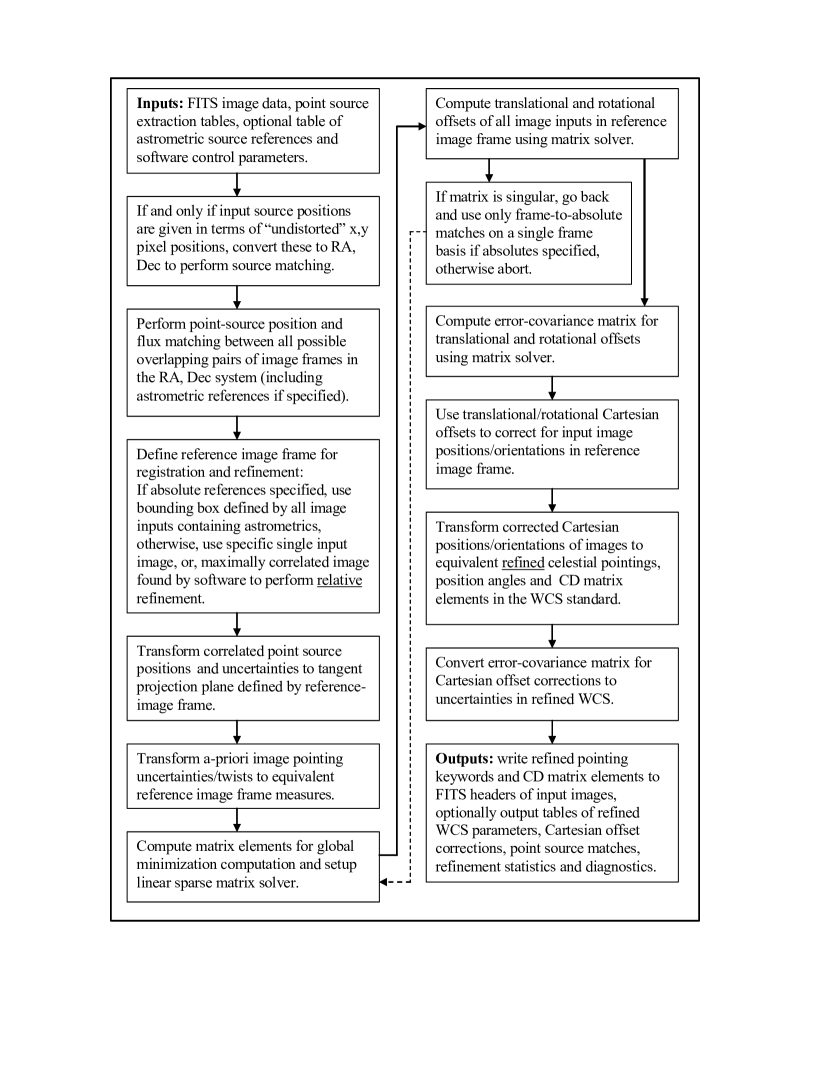
The algorithm has been implemented into a stand-alone software package called pointingrefine. The main inputs to pointingrefine are a FITS image list, with each FITS image containing the standard World Coordinate System (WCS) keywords (Greisen and Calabretta, 2002; Calabretta and Greisen, 2002), an accompanying list of flux-calibrated point-source extraction tables, optional astrometric source list, and configuration parameters. The software expects point source extraction tables adhering to the format generated by the Spitzer Science Center (SSC) source extractor. The complete pointingrefine package is available at http://ssc.spitzer.caltech.edu/postbcd/. This includes programs to perform point source extraction as well, although these will not be described here. A general overview of the processing steps involved in the global minimization algorithm (the heart of pointingrefine) is shown in Figure 1. In the following sections, we expand on some of the more important computational steps of this algorithm.

2.1 Set-up and Point Source Matching

Prior to source matching, we first compute the total number of image-pairs expected to be overlapping (which could potentially contain correlated/common sources) in the input ensemble of images. This is used for efficient a-priori memory allocation. Given a number of images, $N_{imgs}$, the maximum number of distict frame pairs that can mutually overlap is

$$N_{maxpairs}=\frac{1}{2}N_{imgs}\left(N_{imgs}-1\right).$$ (1)

This maximum occurs when all images are stacked more-or-less on top of each other. For a sparse mosaic, this number is smaller and thus puts less of a burden on the required memory. The total number of potential overlapping frame pairs is found by computing the distances between the centers of every image pair and finding whether the distance is less than the typical radius of a circle enscribing an image.

Source positions from all extraction tables (including absolute astrometric references if specified) are sorted in declination. This preconditioning speeds up the source matching procedure, converting it from an $O(N^{2})$ to an approximate $O(N)$ linear process. Every possible overlapping image pair is scanned for common point sources in the RA, Dec coordinate system. Both position and flux matching is performed. The position match step attempts to find sources falling within a nominal search radius (typically several times the root sum squares of prior image pointing uncertainty and extraction centroid error). If more than one match is found within the search radius, no match is declared, due to possible ambiguity. In other words, only singly matched sources within the search radius are used. Sources are also simultaneously matched in flux. A flux match is satisfied if two fluxes fall within a maximum tolerable relative flux difference threshold. The software includes options to re-scale the input fluxes of astrometric references to be commensurate with those of actual extractions. A minimum of two matches per image is enforced to declare a correlated image pair, since this is the minimum required to estimate a rotational offset between the pair unambiguously.

In preparation for the global minimization step (see below), all point source match positions and uncertainties are mapped into the pixel coordinates of a Cartesian reference image frame. The definition of this reference depends on whether absolute or relative refinement is desired. The pointingrefine software distinguishes between these options from its given inputs. Two inputs are required for absolute refinement. First, the software expects a Fiducial Image Frame (FIF). This is a file listing various WCS parameters that define the tangent point and boundary of a “fiducial image” encompassing all images. Second, a list of astrometric (absolute) sources that fall within the FIF boundary is required. The FIF acts as an effective input image whose sources are the astrometric references. Refinement with respect to such a FIF ensures both absolute and relative refinement amongst images. In relative refinement mode, all input images can be registered and refined with respect to a single input image. In this mode, either the software selects an image from the input list which is maximally correlated (has most overlaps) with other images, or the user can specify their own.

2.2 Global Minimization

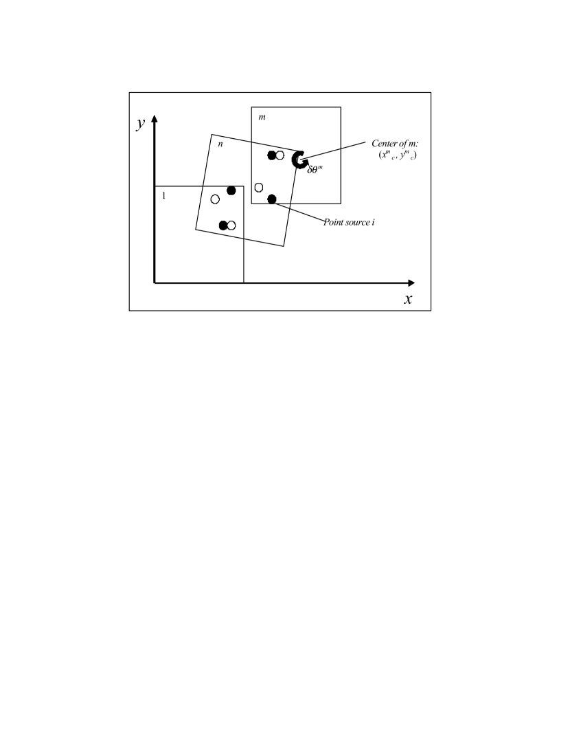
Consider the simple three-image mosaic in Figure 2. Image “1” defines the “fiducial” reference frame. The circles represent point sources detected from each overlapping image pair transformed into the reference frame of image 1. The filled circles are sources extracted from image n and the open circles are sources extracted from either image 1 or m. The matched source pairs are shown offset from each other to mimic the presence of random pointing uncertainty in each input image. These are the offsets we wish to compute and use to correct each frame pointing. A one-dimensional representation of the projection geometry in the reference image frame is depicted in Figure 3. All input images have sizes in the reference frame that depend on their distance from the reference image tangent point. The projected linear size scales with angular distance $\theta_{t}$ as $\>\>\approx 1\>+\>\tan^{2}\theta_{t}$. The pointingrefine algorithm appropriately accounts for the inflation of centroid uncertainties and separations of correlated sources when projected into the reference frame. A potential problem for the algorithm is if image sizes and mosaic extents are large enough to cause a non-uniform dependence in scale over the region in which an input image is projected. The dependence of this effect with $\theta_{t}$, however, is weak. For instance, the projected scale varies by $\lesssim 1\%$ across an image $30\arcmin$ in size at angular distances $\theta_{t}\lesssim 30\arcdeg$.

The main assumption of the algorithm is that the random uncertainty in measured twist angle of an individual image frame ($\delta\theta^{m}$ in Figure 2) is small enough to ensure $\sin\delta\theta^{m}\approx\delta\theta^{m}$ (see below). $\delta\theta\lesssim 1\arcmin$ is a good working measure for the purposes of this algorithm. This is justified for the Spitzer science instruments where the absolute twist angle uncertainty is typically $\lesssim 30\arcsec$ (1-$\sigma$).

In a rectilinear coordinate system (say that defined by the frame of image 1 in Figure 2), the positions of a point source i detected from images m and n are related via the transformation:

$$\left(\begin{array}[]{c}x^{m}_{i}\\ y^{m}_{i}\end{array}\right)\rightarrow\left(\begin{array}[]{c}\tilde{x}^{n}_{i}\\ \tilde{y}^{n}_{i}\end{array}\right)=\left(\begin{array}[]{c}x^{m}_{c}\\ y^{m}_{c}\end{array}\right)+\left(\begin{array}[]{lr}\cos\delta\theta^{m}&-\sin\delta\theta^{m}\\ \sin\delta\theta^{m}&\cos\delta\theta^{m}\end{array}\right)\left(\begin{array}[]{c}x^{m}_{i}-x^{m}_{c}\\ y^{m}_{i}-y^{m}_{c}\end{array}\right)+\left(\begin{array}[]{c}\delta X^{m}\\ \delta Y^{m}\end{array}\right)$$ (2)

where $\delta\theta^{m}$ is a rotational offset, $\delta X^{m}$, $\delta Y^{m}$ orthogonal translations, and ($x^{m}_{c}$ , $y^{m}_{c}$) the center coordinates of image m in the reference image frame. The rotation $\delta\theta^{m}$ is measured in a counterclockwise sense so that a rotation followed by orthogonal translations in x and y of image m will align the sources (open circles) detected therein with those detected in image n.

The assumption of small twist angle uncertainty (see above) implies $\sin\delta\theta^{m}\approx\delta\theta^{m}$ and $\cos\delta\theta^{m}\approx 1$ and thus, the pair of equations defined by (2) can be linearized in $\delta\theta^{m}$ as follows.

$$x^{m}_{i}\rightarrow\tilde{x}^{n}_{i} = x^{m}_{i}-(y^{m}_{i}-y^{m}_{c})\delta\theta^{m}+\delta X^{m}$$

$$y^{m}_{i}\rightarrow\tilde{y}^{n}_{i} = y^{m}_{i}+(x^{m}_{i}-x^{m}_{c})\delta\theta^{m}+\delta Y^{m},$$

where ($\tilde{x}^{n}_{i}$, $\tilde{y}^{n}_{i}$) represents a position, corrected for unknown image rotation and orthogonal translations.

We define a cost function $L$, representing an inverse-variance weighted sum of squares of all matched point-source positional differences from all overlapping image pairs ($m$, $n$):

$$L=\sum_{m,n(n>m)}\sum_{i}\left\{\frac{1}{\Delta x_{i}^{m,n}}[\tilde{x}^{n}_{i}-\tilde{x}^{m}_{i}]^{2}+\frac{1}{\Delta y_{i}^{m,n}}[\tilde{y}^{n}_{i}-\tilde{y}^{m}_{i}]^{2}\right\}\>\>+\>\>L_{apriori}\>\>,$$ (4)

where

$$\Delta x_{i}^{m,n} = \sigma^{2}(x^{m}_{i})+\sigma^{2}(x^{n}_{i})$$ (5)

$$\Delta y_{i}^{m,n} = \sigma^{2}(y^{m}_{i})+\sigma^{2}(y^{n}_{i})$$

and the $\sigma^{2}$ represent variances in extracted point source centroids. The summations in Equation 4 are over all matched point-sources from all image overlaps, including sources matched to any astrometric references present in the FIF if available. The FIF or absolute reference frame (as defined in Section 2.1) is treated as an effective input image when source matching is performed.

The additive term $L_{apriori}$ in Equation 4 represents an “a-priori” weighting function which makes use of actual measured pointing uncertainties of the images. This function is defined as:

$$L_{apriori}\>\>=\>\>\sum_{m,n(n>m)}\left\{\frac{(\delta X^{m})^{2}}{\sigma^{2}_{Xm}}+\frac{(\delta Y^{m})^{2}}{\sigma^{2}_{Ym}}+\frac{(\delta\theta^{m})^{2}}{\sigma^{2}_{\theta m}}+\frac{(\delta X^{n})^{2}}{\sigma^{2}_{Xn}}+\frac{(\delta Y^{n})^{2}}{\sigma^{2}_{Yn}}+\frac{(\delta\theta^{n})^{2}}{\sigma^{2}_{\theta n}}\right\}\>,$$ (6)

where the $\sigma^{2}_{jm}$, $\sigma^{2}_{jn}$ ($j\>=\>X,\>Y,\>\theta$) represent measured pointing variances (in the ICRS) transformed into the reference image frame. The purpose of including $L_{apriori}$ is to avoid over-refining or biasing those images whose inherent measured pointing uncertainties are already small (within nominal requirements). In other words, those images whose uncertainties are known to be small a-priori, will have have a larger contribution to $L_{apriori}$ relative to the correlated source term (double sum in Equation 4). Consequently, the solution will be biased towards minimizing $L_{apriori}$ and not the correlated source term which could potentially degrade expected image offsets (and final refined pointings). In the limit $L\>\rightarrow\>L_{apriori}$, the global minimum will be closer to $\delta\theta\approx\delta X\approx\delta Y\approx 0$. Vice-versa, large pointing uncertainties will bias the solution towards the correlated source term where refinement via point-source matches is obviously needed.

Equation 4 can be rewritten in terms of physical image offsets $\delta\theta^{m}$, $\delta X^{m}$ and $\delta Y^{m}$ for an arbitrary image m via use of Equations 2.2 and 6:

$$L = \sum_{m,n(n>m)}\Biggl{[}\>\sum_{i}\Biggl{\{}\frac{1}{\Delta x_{i}^{m,n}}\left[x^{m}_{i}-(y^{m}_{i}-y^{m}_{c})\delta\theta^{m}+\delta X^{m}-x^{n}_{i}+(y^{n}_{i}-y^{n}_{c})\delta\theta^{n}-\delta X^{n}\right]^{2}\>\>+$$ (7)

$$\frac{1}{\Delta y_{i}^{m,n}}\left[y^{m}_{i}+(x^{m}_{i}-x^{m}_{c})\delta\theta^{m}+\delta Y^{m}-y^{n}_{i}-(x^{n}_{i}-x^{n}_{c})\delta\theta^{n}+\delta Y^{n}\right]^{2}\Biggr{\}}\>\>+$$

$$\frac{(\delta X^{m})^{2}}{\sigma^{2}_{Xm}}+\frac{(\delta Y^{m})^{2}}{\sigma^{2}_{Ym}}+\frac{(\delta\theta^{m})^{2}}{\sigma^{2}_{\theta m}}+\frac{(\delta X^{n})^{2}}{\sigma^{2}_{Xn}}+\frac{(\delta Y^{n})^{2}}{\sigma^{2}_{Yn}}+\frac{(\delta\theta^{n})^{2}}{\sigma^{2}_{\theta n}}\>\Biggr{]}.$$

The cost function defined by Equation 7 can be treated as a standard $\chi^{2}$ statistic to the extent that point source centroid uncertainties are independently random and Gaussian, a good approximation in this case. The probability density function for $L$ about its global minimum is therefore the $\chi^{2}$ distribution for $\nu$ degrees of freedom where

$$\nu\>=\>2N_{matches}-3(N_{imgs}-1).$$ (8)

$N_{matches}$ is the total number of point-source matches in all image overlap regions and $N_{imgs}$ the total number of images containing the detected matches (including the reference image). The total number of parameters to solve is actually $3(N_{imgs}-1)$ since we have three offsets ($\delta\theta^{m}$, $\delta X^{m}$ and $\delta Y^{m}$) for every image m and we exclude the reference image which by definition is constrained to have $\delta\theta=0$, $\delta X=0$ and $\delta Y=0$.

Our aim is to minimize $L$ with respect to all image offsets $\delta\theta^{m}$, $\delta X^{m}$ and $\delta Y^{m}$ for every correlated image m. At the global minimum of $L$, partial derivatives with respect to these three offsets for each image m are required to vanish:

$$\frac{\partial L}{\partial\>\delta\theta^{m}}=0;\>\>\>\>\frac{\partial L}{\partial\>\delta X^{m}}=0;\>\>\>\>\frac{\partial L}{\partial\>\delta Y^{m}}=0.$$ (9)

Evaluating these partial derivatives leads to a set of three simultaneous equations for each image in the ensemble. For $N_{imgs}$, we therefore have $3(N_{imgs}-1)$ simultaneous equations in $3(N_{imgs}-1)$ unknowns. Each image m of an ensemble $m\>=\>1..M$ could be potentially correlated (contain sources in common) with any other image n where $n\>=\>1..N;\>m\>\neq\>n$ and $M\>=N\>=\>N_{imgs}-1$. From the conditions defined in Equation 9, the simultaneous system of equations used to solve for the offsets of all images m, can be represented as the matrix equation:

$$\left(\begin{array}[]{ccccccccc}A^{m=1}_{\theta}&A^{m=1}_{X}&A^{m=1}_{Y}&.&.&.&A^{n=N}_{\theta}&A^{n=N}_{X}&A^{n=N}_{Y}\\ B^{m=1}_{\theta}&B^{m=1}_{X}&0&.&.&.&B^{n=N}_{\theta}&B^{n=N}_{X}&0\\ C^{m=1}_{\theta}&0&C^{m=1}_{Y}&.&.&.&C^{n=N}_{\theta}&0&C^{n=N}_{Y}\\ .&.&.&.&.&.&.&.&.\\ .&.&.&.&.&.&.&.&.\\ .&.&.&.&.&.&.&.&.\\ A^{n=1}_{\theta}&A^{n=1}_{X}&A^{n=1}_{Y}&.&.&.&A^{m=M}_{\theta}&A^{m=M}_{X}&A^{m=M}_{Y}\\ B^{n=1}_{\theta}&B^{n=1}_{X}&0&.&.&.&B^{m=M}_{\theta}&B^{m=M}_{X}&0\\ C^{n=1}_{\theta}&0&C^{n=1}_{Y}&.&.&.&C^{m=M}_{\theta}&0&C^{m=M}_{Y}\\ \end{array}\right)\left(\begin{array}[]{c}\delta\theta^{m=1}\\ \delta X^{m=1}\\ \delta Y^{m=1}\\ .\\ .\\ .\\ \delta\theta^{m=M}\\ \delta X^{m=M}\\ \delta Y^{m=M}\\ \end{array}\right)\>\>=\>\>\left(\begin{array}[]{c}\Psi^{m=1}_{A}\\ \Psi^{m=1}_{B}\\ \Psi^{m=1}_{C}\\ .\\ .\\ .\\ \Psi^{m=M}_{A}\\ \Psi^{m=M}_{B}\\ \Psi^{m=M}_{C}\\ \end{array}\right)$$ (10)

Equation 10 is of the form ${\bf M.X=\Psi}$. Elements of the coefficient matrix ${\bf M}$ and the right-hand-side column vector ${\bf\Psi}$ are given in Appendix A. The solution for the column vector ${\bf X}$ with $3(N_{imgs}-1)$ unknowns can be obtained using linear sparse matrix methods since, depending on the mosaic geometry, a large number of the matrix elements can be zero. In general, the fraction of zeros will be $\geqslant\frac{2}{9}$ ($\gtrsim 22\%$). The $\approx 22\%$ minimum will occur when every image of the ensemble is correlated with every other, such as in a coadded stack. The level of sparsity in ${\bf M}$ will increase with non-zero elements along a block diagonal if one desires to tie and refine images with respect to astrometric absolute references alone. In this specialized case, n = the reference image and all elements with superscript n in ${\bf M}$ will be zero. In general, the minimum and maximum possible number of zeros in the matrix ${\bf M}$ are

$$N_{min} = 2(N_{imgs}-1)^{2}\>\>{\rm and}$$ (11)

$$N_{max} = 9(N_{imgs}-1)^{2}-7(N_{imgs}-1)$$

respectively.

We use the UMFPACK library to solve the matrix equation 10. This is adapted for solving large nonsymmetric matrix systems. The library includes an iterative scheme to correct solutions for the inevitable accumulation in round-off error during the LU-factorization stage.

We also compute the full error-covariance matrix for all image offsets ($\delta\theta^{m}$, $\delta X^{m}$, $\delta Y^{m}$), which is given by the inverse of the coefficient matrix: ${\bf C=M^{-1}}$ (e.g., Press et al. (1999)). Variances in each offset are along the diagonal of ${\bf C}$ and covariances are given by off-diagonal elements. The covariance matrix ${\bf C}$ is computed using the same matrix solver as above by repeatedly solving for each unknown column ${\bf X_{c}}$ in ${\bf M^{-1}}$ such that ${\bf M.X_{c}=I_{c}}$ where ${\bf I_{c}}$ is the corresponding column in the identity matrix. An analysis of the covariance matrix using real data is presented in Appendix B.

Images which are not correlated (lack point source matches) with any others in the input ensemble cannot contribute to the globally minimized cost function $L$. For these images, the pointingrefine software explicitly sets their reference frame offsets to zero and no refinement of their pointing is possible. As a further detail, the inclusion of the a-priori weighting function $L_{apriori}$ (Equation 6) guarantees that the matrix in Equation 10 will be non-singular. The priors provide at least one measurement per image. If these are omitted from the cost function (Equation 4), then there are cases where the matrix could be singular. This can occur if the input image ensemble contains clusters of correlated images disjoint from each other with a non-contiguous/broken path existing between the clusters. This situation leads to an under-represention of images across the full simultaneous system of equations and the determinant will be zero. As indicated in the processing flow of Figure 1, if this occurs in absolute refinement mode, a second pass computation is attempted and only those frames which contain absolute astrometric matches are used. No relative frame-to-frame information is used and images are refined based on their absolute source content alone. The matrix effectively becomes block diagonal and a non-zero determinant is guaranteed. In relative refinement mode, no attempt is made to perform registration within each disjoint sub-ensemble. Instead, the software will abort with a message indicating that disjoint clusters exist.

Once image offset corrections ($\delta\theta^{m}$, $\delta X^{m}$, $\delta Y^{m}$) and associated uncertainties have been determined in the reference image frame, the final step involves refining the celestial pointing and orientation of each image m. This is performed by correcting the pointing centers ($x^{m}_{c}$, $y^{m}_{c}$) of each image in the reference image frame via Equation 2.2, i.e.,

$$x^{m}_{c}(new) = x^{m}_{c}(old)+\delta X^{m}$$ (12)

$$y^{m}_{c}(new) = y^{m}_{c}(old)+\delta Y^{m}$$

and then transforming back to the sky to yield refined pointings in the ICRS. Image orientations are refined in a similar manner. For these, we correct and transform two fiducial points per image to determine uniquely the refined position angle. The main outputs of the pointingrefine software are additional WCS keywords written to FITS image headers representing refined pointings and orientations on the sky (see processing flow in Figure 1).

2.3 Optimization and Expectations

The accuracy in pointing refinement or registration can be severely limited by possible systematics. For example, inaccurately calibrated image scale and/or distortions known a-priori to be position dependent will bias extraction centroids and have adverse affects on the separations of bonafide source matches and hence final globally minimized solutions. A method to test for possible contamination from systematics involves examining distributions of matched source separations after refinement and comparing these with that contributed by (random) centroid uncertainties. This will be performed using real data in Section 4.

The presence of absolute-astrometric point sources are an important ingredient for refinement and registration in general. These reduce the potential for a biased random walk in refined pointing with distance of an image from a fiducial reference. Such effects are also alleviated by using appropriate prior pointing uncertainty information in the global minimization cost function (see Equation 4). Absolute astrometric references provide a set of “anchor points” to which all extractions will be attracted. If one desires to perform absolute refinement with little or no astrometric references, then sufficient numbers of images are needed to increase the number of potential matches in frame overlap regions for a single point source. This is needed in order to approach a normal distribution about the expected absolute source position. In other words, large numbers of correlated source positions will ensure that the mean position of a correlated source cluster is close to the “truth”, or that which will result after refinement (assuming no systematics as discussed above). Due to the rarity of cases with numerous image overlaps providing good normally-distributed sampling, it is advised to use astrometric references wherever possible.

The accuracy to which we can refine the pointings of an ensemble of mutually correlated images predominately depends on the number of point source matches available (both relative and absolute). With randomly distributed uncertainties in point source centroids, it is expected that the mean separation between matched source positions is approximately Gaussian after refinement, by virtue of the central limit theorem. In this limit, the (radial) uncertainty in refinement of a single image will scale as

$$\sigma_{r}\simeq\sqrt{\frac{\sigma_{ext}^{2}+\sigma_{abs}^{2}}{\frac{N_{ext}}{2}\left[1+\left(\frac{\sigma_{abs}^{2}}{\sigma_{ext}^{2}}\right)\right]+N_{abs}}},$$ (13)

where $N_{ext}$ and $N_{abs}$ represent respectively the number of frame-to-frame and frame-to-absolute source match pairs in all overlap regions associated with the image, $\sigma_{ext}$ is a typical source extraction centroid uncertainty, and $\sigma_{abs}$ is an astrometric source position uncertainty. This approximation assumes that $\sigma_{ext}>0$ or $\sigma_{abs}>0$ when either $N_{ext}>0$ or $N_{abs}>0$ respectively. For no astrometric matches, we set $N_{abs}=0$ and $\sigma_{abs}=0$, and Equation 13 reduces to $\sigma_{ext}\sqrt{2/N_{ext}}$. We expect to measure source extraction centroids to better than $\approx 0.1$ pixel, ($\approx 0.121\arcsec$ for Spitzer’s IRAC focal plane arrays). If we assume for example astrometric positional errors of $\approx 0.2\arcsec$ (conservatively speaking), then to refine image pointings to an accuracy better than $\approx 0.1\arcsec$ will require at least five astrometric point-source matches per frame if $N_{ext}=0$, or less, if $N_{ext}>0$. One can see that with more point-source matches, the better the refinement. This assumes the observational setup allows for sufficient frame-to-frame overlap to ensure good numbers of relative matches $N_{ext}$. If this is not the case, one will have to resort to using pure astrometric (absolute source) matches alone.

To summarize, corrections for optimal refinement will effectively be given by the magnitude of frame pointing uncertainties with errors approximated by Equation 13. The latter assumes that in the limit of increasing number of matches, the mean source separation per image overlap region is approximately normally distributed with an uncertainty determined exclusively by point source centroid uncertainties. Any position-dependent systematic offset between source matches such as nonuniform pixel scale or inaccurately calibrated distortion will limit the refinement accuracy to the size of systematic error involved.

3 Validation Against a Monte-Carlo Simulation

We quantitatively assess the performance of the above algorithm using a simulation of 1000 mosaicked images, with each image’s coordinates modeled with an uncertainty drawn from a Gaussian distribution. The simulation is generic in that it represents a good overall representation of the type of data that could be acquired with modern optical/near-infrared detectors to moderately faint magnitudes ($m_{opt}\simeq 23$ or $m_{nearIR}\simeq 19$). To facilitate a comparison with real observations in Section 4, we have chosen to model the source count distribution and detector properties with that expected (and more or less observed) in the $3.6\micron$ band of Spitzer’s IRAC instrument. A more detailed description will be given in Section 4.

The “truth” source flux-density distribution was simulated using the models of Xu et al. (2003). These assume a high galactic latitude stellar model, several galaxy luminosity functions depending on galaxy morphological type, and exploit a large library of spectral energy distributions. This simulation was used extensively for predicting Spitzer source populations (Lonsdale et al., 2003) and for validating processing pipelines.

The simulation steps are as follows.

1. A “truth” list of random source flux densities was generated using the models of Xu et al. (2003) covering an area of  0.45 square degrees down to a flux density of $10\mu$ Jy at $3.6\micron$ (equivalent to $\simeq 18.6$ magnitudes in the Vega system).

2. Truth sources were assigned both random and correlated positions within the area to be mosaicked. Galaxies were assumed to have a weak correlated component with amplitude (excess above random) based on an empirical $K$-band 2-point angular correlation function: $w(\theta)\simeq 0.001(\theta/{\rm deg})^{-0.8}$. A pixel scale of $\approx 1.21\arcsec$ (characteristic of the IRAC arrays) was used when mapping sources to the pixel frame of the mosaic.

3. Truth sources were convolved with a point spread function (PSF) scaled by the appropriate source flux. PSF-convolved truth sources were mapped into the mosaic frame with no pixel resampling.

4. 1000 ($256\times 256$ pixel) “truth image” frames were generated from the full mosaic area using a dither and mapping strategy which assumed $\approx 60\%$ adjacent image overlap. The optimal map geometry for this 1000-image set was generated by D. Shupe (2002, SSC, private communication). RA, Dec, and Twist angle information is also attached to each image at this stage.

5. A new set of 1000 images was generated (our simulated control sample) with uncertainties added to image pointings and position angles. Pointing offsets (prior uncertainties) were modeled as Gaussian random deviates along each independent orthogonal image axis. These were drawn from a zero-mean Gaussian distribution with $\sigma=0.85\arcsec$ per axis. This choice for $\sigma$ is based on a pre-launch pointing knowledge of $\sim 1.2\arcsec$ (1-$\sigma$ radial) for Spitzer in the science instrument frame. Even though Spitzer can now actually do better than this by a factor of $\sim 1.5$ (Section 4), the ultimately refined pointings are independent of the magnitude of reasonable simulated prior uncertainty assumed (see below). Twist angle uncertainties were modeled as Gaussian with $\sigma=20\arcsec$. A smoothly varying background adjusted with the expected Poisson and (IRAC band-1) read-noise per pixel was added to each image.

6. An absolute source list (representing astrometric references) was generated by taking the brightest truth sources which gave a mean density of $\simeq 50$ sources per $5.2\arcmin\times 5.2\arcmin$ image region. This resulted in 3030 truth sources. To imitate an astrometric catalog, the sources were assigned with positions modeled as $truth\pm u.\sigma$ along each axis with $u$ drawn from a Gaussian distribution with $\sigma=0.06\arcsec$. This is typical for sources in the 2MASS point source catalog to $K_{s}\simeq 15$ (see Section 4 for details regarding the 2MASS catalog).

7. The SSC point source extractor was used on each simulated (control) image to extract sources above a threshold of $5\sigma$. This resulted in $\approx 40$ extractions per frame.

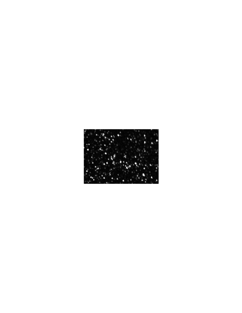
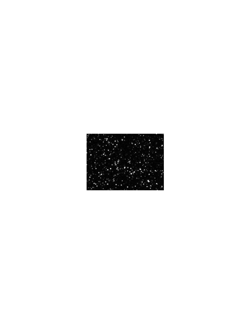
The pointingrefine software was executed on the 1000 image control sample. A source match radius of $3.5\arcsec$ was used to comfortably accomodate prior image pointing errors and extraction centroid errors (typically $0.15\arcsec$ 1-$\sigma$ per axis). Simultaneous flux matching was also applied between frame-to-frame and frame-to-absolute (astrometric) matches with maximum flux difference thresholds of 5 and 10% respectively. A zoomed-in ($2.8\arcmin\times 3.8\arcmin$) section of our 1000-image simulation (with image pointing errors) is shown in the left panel of Figure 4. On the right is the same section after pointing refinement. The increase in resolution is dramatic. There is a factor of $\sim 6$ decrease in mean source match separation leading to more localized point source flux distributions and detectability to fainter levels. In this test, the surface brightness is increased by factors of $\sim 2-3.5$ for detected sources after refinement. This is as expected given that the 1-$\sigma$ radial image pointing uncertainty is of the order the input pixel size, and the instrinsic PSF has FWHM $\simeq 1.66\arcsec$.

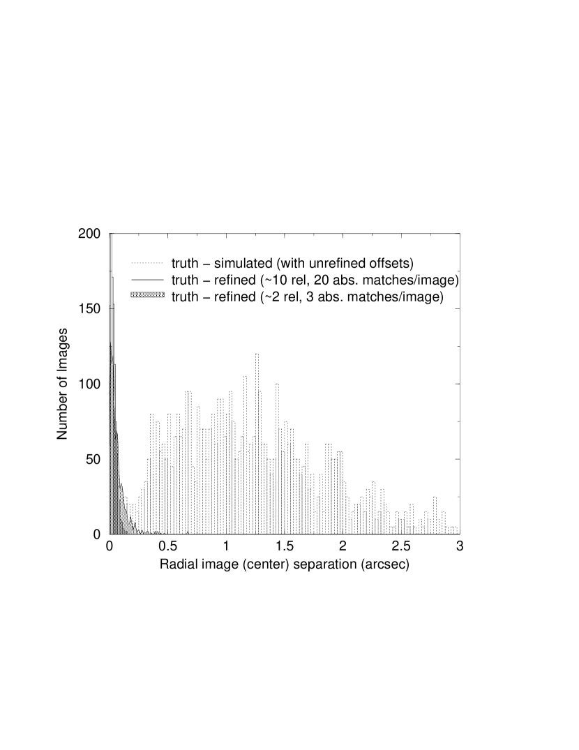
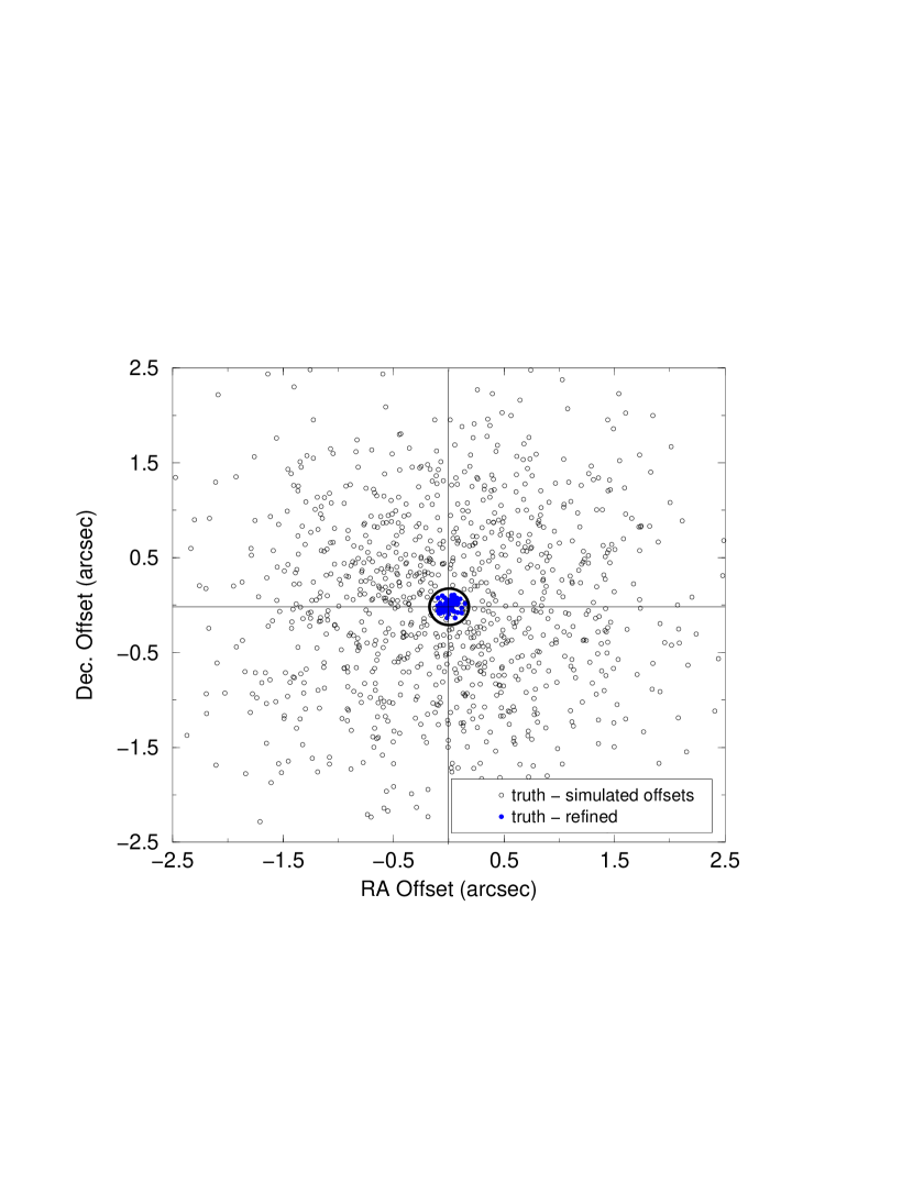
To get a more quantitative assessment of the performance of pointingrefine, we compare the distribution of separations between image center pointings of “truth” and simulated (control sample) images before and after refinement. This is shown in the top panel of Figure 5. Two different runs of pointingrefine were performed based on the number of (brightest) extractions used per image. One gave an average of $\sim 10$ relative (frame-to-frame) and $\sim 20$ absolute-astromeric source matches per image (the “10/20-match” case), and the second resulted in an average of $\sim 2$ relative and $\sim 3$ absolute matches per image (the “2/3-match” case). It should be noted that two matches per image is the absolute minimum to determine unambiguously two orthogonal shifts and an orientation per frame (i.e. the number of degrees of freedom (#dof) $=2N_{matches}-3=1$). The dispersion in image separation relative to truth after refinement for the “10/20-match” case is $\simeq 65$ mas (1-$\sigma$ radial). For the “2/3-match” case, this is $\simeq 110$ mas. For the given match statistics, these numbers are more or less consistent with the simple scaling relation given by Equation 13. Offset distributions along each axis are shown in the lower panel of Figure 5 where the open circle represents the 2-$\sigma$ contour for the “2/3-match” case.

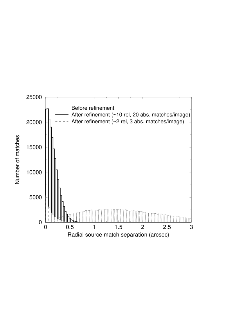
By comparing differences in image radial separations before and after refinement, we find that over 890 images have their pointing refined to better than 95% relative to “truth” (for the “10/20-match” case). The top panel in Figure 6 shows the distribution in fractional refinement. This quantity is defined as the ratio of separations: $1-{\rm D}(refined-truth)/{\rm D}(unrefined-refined)$. For the “2/3-match” case, slightly less than half have the same amount of refinement, although most images are refined to better than 80%, corresponding to a discrepancy of $\simeq 180$ mas within truth image positions. Thus the refinement is very good, even with minimal matches.

The bottom panel in Figure 6 shows distributions in matched source radial separations before and after refinement. Uncertainties in both image pointing and source extraction centroids (or radial separation) contribute to the dispersion in the unrefined distribution. Image pointing uncertainties dominate, with a $1.2\arcsec$ contribution compared to $\simeq 0.2\arcsec$ for extraction centroids (both 1-$\sigma$ radial). After pointing refinement, the dispersion in radial source separation is expected to be dominated exclusively by extraction centroid errors and indeed, the distributions confirm this for both the “2/3” and “10/20-match” case (Figure 6 bottom left). The distribution for the “2/3-match” case is narrower since such matches were performed using the brightest extractions per image, and these inherently have better determined centroids.

The separation between two source extraction centroids ($x_{i},\>y_{i}$) and ($x_{j},\>y_{j}$) is given by

$$r\>=\>\left[(x_{i}-x_{j})^{2}+(y_{i}-y_{j})^{2}\right]^{1/2}.$$ (14)

Since a majority of extractions are unresolved point sources with very circular error-ellipses, we can ignore any correlations between uncertainties along each axis. To a good approximation, the uncertainty in radial separation between any two centroids can therefore be written:

$$\sigma_{r}\>\simeq\>\sqrt{\sigma_{x_{i}}^{2}+\sigma_{x_{j}}^{2}}\>\simeq\>\sqrt{\sigma_{y_{i}}^{2}+\sigma_{y_{j}}^{2}},$$ (15)

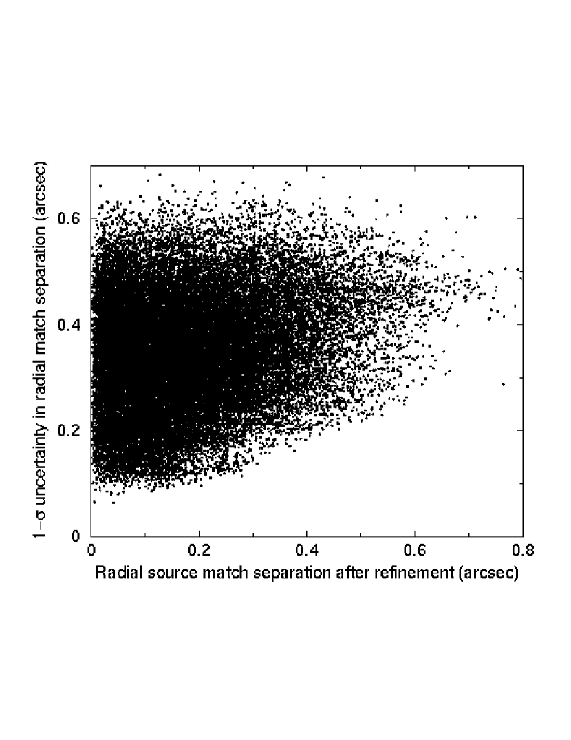
where ($\sigma_{x_{i}}^{2},\>\sigma_{y_{i}}^{2}$) and ($\sigma_{x_{j}}^{2},\>\sigma_{y_{j}}^{2}$) are centroid variances in each axis for sources $i$ and $j$ respectively. A comparison between uncertainties in matched source radial separation (Equation 15) and actual separations (Equation 14) after refinement is shown in the top panel of Figure 7 (for “10/20-match” case). They are both mutually consistent, although the spread is greater at separations $\lesssim 0.3\arcsec$. After refinement and in the absence of systematics, any residual separation in a matched source pair must be due to intrinsic centroiding error alone. Since separations between matched sources along each axis are to a good approximation independently random and normally distributed with zero mean ($\langle x_{i}-x_{j}\rangle\simeq\langle y_{i}-y_{j}\rangle\simeq 0$), the quantity $r$ (Equation 14) can be shown to follow a $\chi$ distribution with two degrees of freedom (e.g., Evans et al. (2000)). This special case is also known as the Rayleigh distribution:

$$P(r)\>=\>\frac{r}{\beta^{2}}\exp{\left[-\frac{1}{2}\left(\frac{r}{\beta}\right)^{2}\right]},$$ (16)

where $\beta$ is a parameter characterizing the width. This can be written in terms of the second moment (variance) of $P(r)$ as follows

$$\beta\>=\>\sqrt{\left(\frac{2}{4-\pi}\right)\sigma_{r}^{2}}\>\simeq\>1.52\>\sigma_{r}\>.$$ (17)

For a given uncertainty $\sigma_{r}$ as computed from Equation 15, the variation in the density of points with $r$ along any horizontal cut in Figure 7 is qualitatively consistent with that predicted by Equations 16 and 17.

The bottom panel of Figure 7 shows the dependence of the reduced $\chi^{2}$ (effectively the cost function in Equation 7 divided by number of degrees of freedom defined by Equation 8.) as a function of increasing number of images $N_{i}$ in our 1000-image simulation. It’s important to note that image offsets are not re-computed using repeated global minimizations for each new set of images $N_{i}$. Instead, the original full 1000-image solution of image offsets is used throughout to re-compute $\chi^{2}$ from Equation 7 as $N_{i}$ is increased for all image pairs ($m,\>n$) such that $n<m\leq N_{i}$. As one approaches the full image set of $N_{i}=1000$, one expects the reduced $\chi^{2}$ to converge to unity if, on average, residuals in source separations after refinement are purely consistent with extraction centroid uncertainties. The lower reduced $\chi^{2}$ values for smaller image numbers (and particularly for all image numbers in the “2/3-match” case) is due to the nonlinear behavior in $\chi^{2}$ when the number of degrees of freedom is small. Better fits (smaller $\chi^{2}$) can be obtained for very low numbers of degrees of freedom. In Figure 7 (bottom panel), only the “10/20-match” case (with absolute refinement as studied above) shows approximate covergence to one, and the other curves are not far from it. Also shown is a case where only relative frame-to-frame matches and no astrometric references are used. This case tends to show a slightly higher reduced $\chi^{2}$ ($\simeq 1.04$), which is significant since it is almost 20 standard deviations from the expected value in reduced $\chi^{2}$ ($\sigma_{\chi^{2}}=\sqrt{2/{\rm\#dof}}$, where #dof$=308935$). This was traced as being due to slightly under-estimated undertainties in extraction centroids. This is not seen in the absolute refinement case (solid curve) since absolute astrometric uncertainties are themselves over-estimated and their (almost equal) contribution tends to lower the effective $\chi^{2}$ when combined with relative frame-to-frame matches.

To summarize, we have presented a simulation to ascertain the performance of the pointingrefine algorithm. The model-dependent parameters entering our simulation can be isolated to properties of $3.6\micron$ source populations, specifics of the IRAC band-1 array, such as PSF and pixelization, and a-priori telescope pointing knowledge. These can be appropriately rescaled to model other wavelengths and detectors. However, in the absence of systematics in the locations of potential matches between frames (both absolute and relative), and regardless of instrumental setup or detecter properties, the accuracy in refined pointing is purely dictated by the accuracy of point source centroids and match statistics. Our simulation (Figures 5 and 6) indeed shows that the refined pointing will typically never be worse off than the (combined) centroid uncertainties of matched pairs of sources. A well sampled and characterized PSF is expected to give centroiding accuracies to better than one-tenth of a resolution element. If errors are independently random, good match statistics can then only work in our favor to give the desired $\sim 1/\sqrt{N_{matches}}$ improvement in pointing accuracy.

4 Testing on Spitzer-IRAC Data

The Infrared Array Camera (IRAC) is one of three focal plane instruments on the Spitzer Space Telescope (Fazio, 2004). IRAC provides simultaneous $\sim 5.2\arcmin\times 5.2\arcmin$ images at 3.6, 4.5, 5.8 and $8\micron$ (bands 1-4). All four detector arrays in the camera are $256\times 256$ pixels in size, with a pixel size $\simeq 1.2\arcsec$. We present here the results of a case study of observations acquired with IRAC during the in-orbit checkout period (Oct. 2003). In this section, we validate the pointing performance of IRAC and estimate the accuracy of refinement that can be achieved using a standard astrometric catalog and comparisons with our simulation of the $3.6\micron$ band from Section 3.

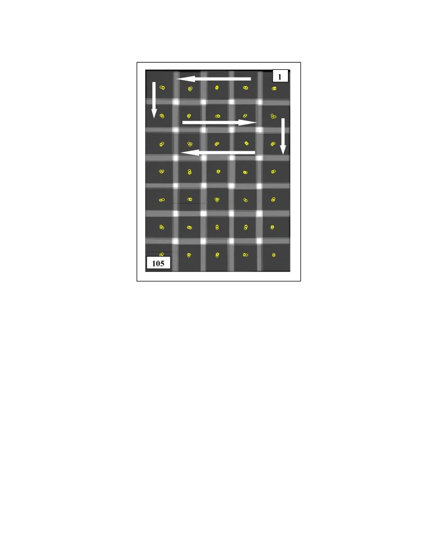
The observational request used for our case study consists of 105 regularly spaced images arranged in a rectangular raster pattern. The coverage map and geometry is shown in Figure 8. Adjacent images have $\sim 20\%$ overlap in each axis, with a coverage of 6 and 12 pixels at the edges and (inner) corners respectively. The mapping was performed in repetitive horizontal scans as shown by arrows in Figure 8. The first image is at top right and the last at bottom left. All images across all bands were preprocessed for removal of instrumental signatures using the SSC’s IRAC pipeline and raw pointing information was attached to FITS headers. Source extraction was then performed using the SSC source extractor with PSFs characterized from in-flight data. Sources were extracted to a uniform signal-to-noise ratio of $5\sigma$ in each band, resulting in an average of $\sim 39$, 24, 13 and 6 extractions per image for bands 1, 2, 3 and 4 respectively. Errors in flux-weighted centroids were on average $\sim 0.18$, 0.22, 0.26 and $0.27\arcsec$ (1-$\sigma$ radial) for each band respectively.

We used data from the Two-Micron All Sky Survey (2MASS) to define a standard astrometric catalog for all IRAC bands. Zacharias et al. (2003) used the USNO CCD Astrograph Catalog (UCAC) (which is accurate to $\sim 20$ mas) to perform an assessment of the accuracy of 2MASS astrometry. They found random errors of 2MASS positions of $\sim 85$ to 140 mas radial to a limiting $K_{s}$ magnitude of 15. We use astrometric sources detected in the 2MASS $K_{s}$ band ($2.12\micron$) which is well suited to IRAC, and as a good working measure, we impose a magnitude limit of $K_{s}=15$. To this limit and at the highest galactic latitudes ($|b|>60\arcdeg$), one expects to find at least two astrometric sources per $\sim 5.2\arcmin\times 5.2\arcmin$ IRAC field $\sim 60\%$ of the time. In the galactic plane anti-center, this increases to at least 30 sources 80% of the time (J. Surace 2000, SSC, private communication).

Using source extractions and astrometric references, the pointingrefine software was executed on each of the four, band-dependent 105-image ensembles. Guided by a post-facto analysis of typical source separations and flux differences, point-source matching was performed using a nominal search radius of $2\arcsec$ and simultaneous flux matching performed with relative (frame-to-frame) and astrometric (frame-to-absolute) flux difference thresholds of 4% and 50% respectively across all bands. Flux matching thresholds were set conservatively high to account for relative and absolute photometric calibration errors and instrinsic scatter between source populations detected in the 2MASS and IRAC bands. Relative and astrometric match statistics are summarized in Table 1.

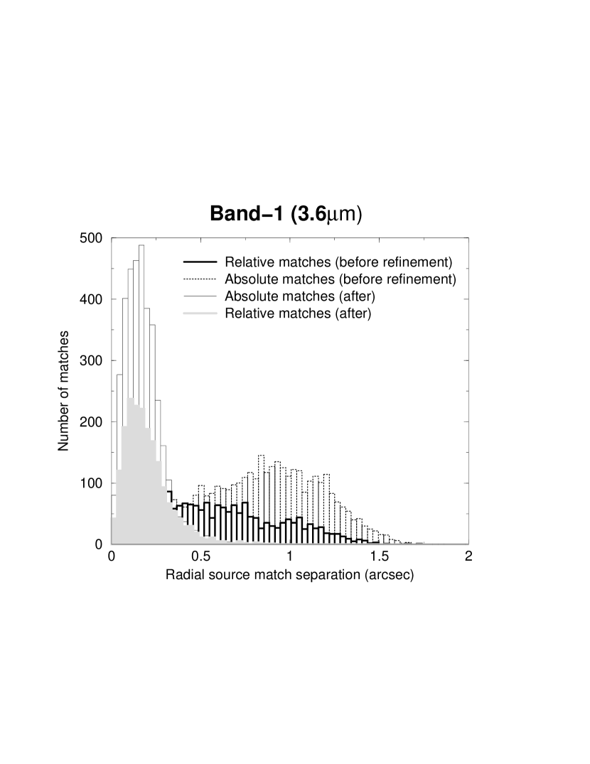
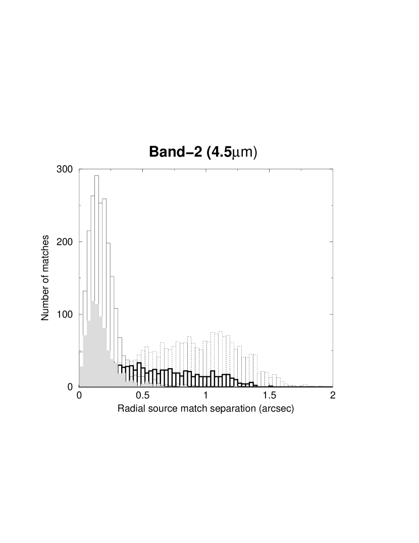
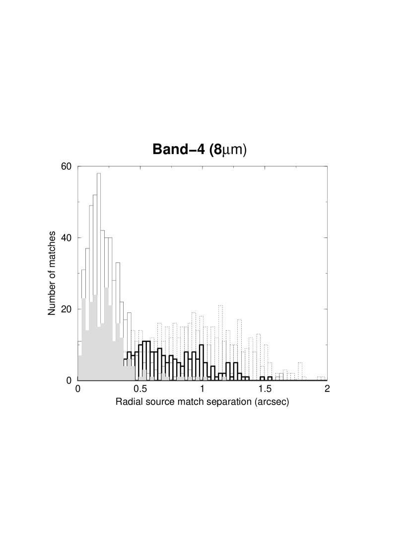
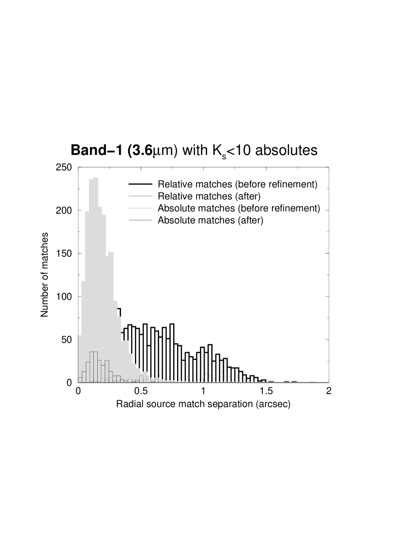
Figure 9 shows distributions in matched source radial separations before and after refinement for all bands. Relative and astrometric matches have been separated. These distributions provide a powerful diagnostic with which to assess the in-flight pointing performance in the IRAC science instrument frame. The end-to-end pointing accuracy is a function of the inherent star-tracker accuracy, the spacecraft control system, how well the star-tracker bore-sight is known in the telescope pointing frame and focal plane array (science instrument) frame, and variations in these due to thermo-mechanical deflections. Spitzer’s star-tracker assembly alone provides pointing and control to better than $0.3\arcsec$ absolute accuracy. The In-Orbit-Checkout (IOC) dataset analyzed here may have additional error sources because the images were obtained while the Spitzer pointing and data-acquisition systems were still being tuned and because the image integration times were very short (1.2 seconds). For example, if the estimate of the time needed for the spacecraft pointing system to “settle” were slightly too short (i.e., underestimated), then the images would have been taken while the spacecraft pointing was changing slightly, providing an additional error term in the pointing transfer. More standard images with relatively long integration times would be much less affected by this source (as long as the settle time is small relative to the integration time). Therefore, the pointing accuracy we derive for this dataset may not be typical for Spitzer, but it still provides a valid test of the POINTINGREFINE algorithm.

We can get an estimate of both the relative and absolute raw pointing for this IRAC dataset from the “before refinement” (dotted and thick lined) histograms in Figure 9. The main difference between bands is in the number of point source matches. Other than that, ranges in radial distributions are more or less consistent. Across all bands, the 1-$\sigma$ radial separation between frame-to-absolute matches is $\sim 0.85$ to $0.93\arcsec$ , while for relative (frame-to-frame) matches, this is $\sim 0.61$ to $0.65\arcsec$ (See Table 1). In addition to actual pointing dispersion, these estimates include a dispersion component from point source centroid errors. The contribution from centroiding error to the “before refinement” distributions however is negligible. Taking for instance the band-1 average centroiding error of $\sim 0.18\arcsec$ and $\sim 0.085\arcsec$ for 2MASS (1-$\sigma$ radial), this translates to effective match separation uncertainties of $\sim 0.14$ and $\sim 0.18\arcsec$ for frame-to-absolute and frame-to-frame (relative) matches respectively, assuming errors in each axis are uncorrelated (see Equation 15). This implies that the actual absolute and relative pointing for the frames in this observation is typically $\sqrt{0.85^{2}-0.14^{2}}\approx 0.83\arcsec$ and $\sqrt{0.61^{2}-0.18^{2}}\approx 0.58\arcsec$ (1-$\sigma$ radial) respectively. Similar results are found using other bands. We should emphasize that these estimates are strictly valid for this dataset alone. They are not representative of the actual pointing performance of IRAC where the absolute pointing is typically $\sim 0\arcsec.45$-$0\arcsec.66$ (1-$\sigma$ radial). For an in-depth study, see Barmby and Lacy (2004).

The source separation distributions after refinement in Figure 9 allow us to validate how well (or whether) images were refined to within accuracies determined by source extraction centroids. As found in our simulation (Figure 5), images were refined to better than $\simeq 65$ mas (1-$\sigma$ radial) within truth pointings, with a corresponding $\simeq 200$ mas dispersion in source separations after refinement (Figure 6). The top panel in Figure 10 shows the distribution of uncertainties in radial match separation (from Equation 15) as a function of separation $r$ for band-1 after refinement. These are broadly consistent above the minimum cut-off uncertainty of $\sim 100$ mas imposed by the finite size of the PSF. The distribution in $r$ at any given uncertainty cut $\sigma_{r}$ can also be described by a Rayleigh distribution (see Equations 16 and 17). Furthermore, Figure 10 shows that typical systematic uncertainties due to inaccurately calibrated distortion are minimal, and if present, are expected to be much less than the centroiding errors. Guided by the simulation in Section 3 and Figure 9, we conservatively conclude that the majority of image pointings must be refined to better $\simeq 200$ mas. In fact, we can predict the absolute dispersion in image pointings about truth using Equation 13. Given the typical match statistics listed in Table 1 and centroiding errors of $0.18\arcsec$ and $0.27\arcsec$ for bands 1 and 4 respectively, we expect dispersions of $\sim 35$ and $\sim 140$ mas (1-$\sigma$ radial) about truth for these bands respectively. We expect these dispersions to be smaller once centroiding errors are brought down using better characterized PSFs.

In this case study, the number of astrometric (frame-to-absolute) matches are factors 1.5 to 2 times greater than relative (frame-to-frame) matches (see Table 1). This is due to the specific flux difference thresholds used in source matching (4% and 50% for relative and absolute matches respectively; see above). The results of Figure 9 assumed 2MASS point sources with $K_{s}\leq 15$. To ascertain the degree to which the number of absolute matches control the level of refinement, we repeated the source matching and refinement for band-1 using a 2MASS magnitude cut of $K_{s}=10$. The bottom panel of Figure 10 shows source separations before and after refinement. The number of absolutes per frame was randomly distributed between 0 and 4 (compared to $\sim 20$ relative matches/frame). When frame-to-absolute separations after refinement are considered alone (open histogram at bottom left), the mean separation is smaller by a factor of $\sim 2$ compared to the $K_{s}\leq 15$ case (top left panel of Figure 9). This is due to inherently lower positional uncertainties for the brighter ($K_{s}\leq 10$) sources. When combined with relative matches however, the mean source separation and hence level of refinement is essentially unchanged compared to our results above.

5 Discussion and Conclusions

We have presented a generic algorithm to perform astronomical image registration and pointing refinement. It is generic in the sense that it can be used on any set of astronomical images which recognize the FITS and WCS pointing standards (Greisen and Calabretta, 2002; Calabretta and Greisen, 2002). Either relative (self-consistent frame-to-frame registration), single image absolute-astrometric, or simultaneous (relative and absolute) refinement is supported. The crux of the method involves matching point source positions between overlapping image frames and using this information to compute image offset corrections by globally minimizing a weighted sum of matched point-source positional differences.

To ensure robust registration and refinement, the algorithm is best optimized with the following criteria.

1. The random uncertainty in measured twist angle of an individual image frame ($\delta\theta$) is assumed to be small such as to ensure $\sin{\delta\theta}\approx\delta\theta$. $\delta\theta\lesssim 60\arcmin$ is a good working measure for the intended applications of this algorithm (where $1-\frac{\sin{\delta\theta}}{\delta\theta}\lesssim 10^{-4}$).

2. Input images have been accurately calibrated for distortion and possible nonuniform pixel scale. Any position-dependent systematic offset between source matches will limit the refinement accuracy to the size of the systematic error involved.

3. Sufficient area overlap between adjacent image frames is needed to ensure good match statistics.

4. Availablity of point sources with well defined flux distribution profiles approaching that of the instrument/detector’s PSF. Extended sources will lead to larger centroiding errors.

5. Well characterized PSF(s) for the image(s) at hand. These are crucial for accurate determination of source extraction centroids. If the inherent telescope pointing uncertainty is of order a third or larger than the detector pixel size, centroiding accuracies to better than one-tenth of a pixel or resolution element are recommended. For pointing uncertainties much less than the pixel size, there is little to be gained in resolution by improving the registration.

6. With the suggested centroiding accuracy from step 5, at least five relative (frame-to-frame) and five absolute source matches per frame will give pointings refined to better than three-hundreths of a pixel (rms). The greater the number of matches, the better the refinement. A minimum of two source matches per image frame, either relative, absolute, or both is required to determine all offset parameters per image unambiguously.

7. Astrometric (absolute) reference sources should be used wherever possible. These provide a baseline to counteract any systematic deviations from “truth”, or expected pointing in the ICRS, especially if absolute refinement is desired.

8. It is assumed that uncertainties in image pointing and point source extraction centroids are random and independent. Prior image pointing uncertainties should be used if available. These will prevent from erroneously over-correcting the pointing for cases in which it is well known a-priori.

Our simulations show that potentially good refinement can be obtained with minimal requirements. For a large fraction of images in an ensemble, refinements of better than $\simeq 65$ mas (1-$\sigma$ radial from truth) can be obtained with an average of $\sim 10$ relative and $\sim 20$ absolute matches per frame with extraction centroids $\lesssim 0.2\arcsec$. This amounts to an improvement of 95% relative to truth for a majority of images. This could be better with higher match statistics and/or more accurate centroids, since typically the 1-$\sigma$ dispersion about truth scales as $\sim\sigma_{ext}\sqrt{2/N_{ext}}$ for a given centroiding uncertainty $\sigma_{ext}$ and number of matches $N_{ext}$.

Analysis of observations from Spitzer’s IRAC instrument shows that the dispersion in source separations after refinement is entirely consistent with the inherent dispersion in extraction centroid uncertainties. This implies that systematic uncertainties such as inaccurately calibrated distortions are negligible, since otherwise dispersions in matched source separations after refinement would be larger relative to centroiding errors. Comparing dispersions of refined pointings about truth with matched source separations as found in our simulation, and rescaling to the appropriate numbers of matches using $1/\sqrt{N_{match}}$ scaling, we predict (at the $2\sigma$ level) refinements to better than $\sim 70$ mas and $\sim 280$ mas for IRAC bands 1 and 4 respectively. These bands bracket two extremes in available source matches, and these refinement estimates correspond to $\sim 55$ and $\sim 8$ (astrometric and relative) matches per band-dependent frame respectively.

The goal of astronomical image registration is to exploit the resolution capabilities of existing and upcoming detectors whose pointing control and stability may not evolve at the same rate. The aim is to optimize the achievable signal-to-noise and science return therein. The algorithm presented herein is just the tip of the iceberg at exploring one of many optimization techniques used in the diverse fields of image and signal processing and computer vision science.

Appendix A Elements of the Coefficient Matrix

In this section, we provide general analytic expressions for elements of the coefficient matrix ${\bf M}$ (Equation 10). These elements are obtained by applying the minimization conditions (Equation 9) to the cost function defined by Equation 7. The “base” coefficent labels $A$, $B$ and $C$ correspond to the three equations obtained by evaluating the partial derivatives in Equation 9 (labelled equations $A$, $B$ and $C$ from left to right respectively). Position and uncertainty variables appearing in the expressions below were defined in Section 2.2.

$$A^{m}_{\theta} = \sum_{n}\sum_{i}\frac{(y^{m}_{i}-y^{m}_{c})^{2}}{\Delta x_{i}^{m,n}}+\frac{(x^{m}_{i}-x^{m}_{c})^{2}}{\Delta y_{i}^{m,n}}+\sum_{n}\frac{1}{\sigma^{2}_{\theta m}}$$ (A1)

$$A^{m}_{X} = -\sum_{n}\sum_{i}\frac{(y^{m}_{i}-y^{m}_{c})}{\Delta x_{i}^{m,n}}$$ (A2)

$$A^{m}_{Y} = \sum_{n}\sum_{i}\frac{(x^{m}_{i}-x^{m}_{c})}{\Delta y_{i}^{m,n}}$$ (A3)

$$A^{n}_{\theta} = -\sum_{n}\sum_{i}\frac{(y^{m}_{i}-y^{m}_{c})(y^{n}_{i}-y^{n}_{c})}{\Delta x_{i}^{m,n}}+\frac{(x^{m}_{i}-x^{m}_{c})(x^{n}_{i}-x^{n}_{c})}{\Delta y_{i}^{m,n}}$$ (A4)

$$A^{n}_{X} = \sum_{i}\frac{(y^{m}_{i}-y^{m}_{c})}{\Delta x_{i}^{m,n}}$$ (A5)

$$A^{n}_{Y} = -\sum_{i}\frac{(x^{m}_{i}-x^{m}_{c})}{\Delta y_{i}^{m,n}}$$ (A6)

$$B^{m}_{\theta} = A^{m}_{X}$$ (A7)

$$B^{m}_{X} = \sum_{n}\sum_{i}\frac{1}{\Delta x_{i}^{m,n}}+\sum_{n}\frac{1}{\sigma^{2}_{Xm}}$$ (A8)

$$B^{n}_{\theta} = \sum_{i}\frac{(y^{m}_{i}-y^{m}_{c})}{\Delta x_{i}^{m,n}}$$ (A9)

$$B^{n}_{X} = -\sum_{i}\frac{1}{\Delta x_{i}^{m,n}}$$ (A10)

$$C^{m}_{\theta} = A^{m}_{Y}$$ (A11)

$$C^{m}_{Y} = \sum_{n}\sum_{i}\frac{1}{\Delta y_{i}^{m,n}}+\sum_{n}\frac{1}{\sigma^{2}_{Ym}}$$ (A12)

$$C^{n}_{\theta} = -\sum_{i}\frac{(x^{n}_{i}-x^{n}_{c})}{\Delta y_{i}^{m,n}}$$ (A13)

$$C^{n}_{Y} = -\sum_{i}\frac{1}{\Delta y_{i}^{m,n}}$$ (A14)

$$\Psi^{m}_{A} = -\sum_{n}\sum_{i}\frac{(y^{m}_{i}-y^{m}_{c})(x^{n}_{i}-x^{m}_{i})}{\Delta x_{i}^{m,n}}+\frac{(x^{m}_{i}-x^{m}_{c})(y^{m}_{i}-y^{n}_{i})}{\Delta y_{i}^{m,n}}$$ (A15)

$$\Psi^{m}_{B} = -\sum_{n}\sum_{i}\frac{(x^{m}_{i}-x^{n}_{i})}{\Delta x_{i}^{m,n}}$$ (A16)

$$\Psi^{m}_{C} = -\sum_{n}\sum_{i}\frac{(y^{m}_{i}-y^{n}_{i})}{\Delta y_{i}^{m,n}}$$ (A17)

Appendix B The Error-Covariance Matrix

The full error-covariance matrix is one of the by-products of the pointingrefine software. This reports all variances and covariances for and between all (inter and intra) image offsets necessary for refinement from the global minimization. It can be used to explore the strength of long-distance correlations between images in a mosaic and the presence of any undue systematic walks after refinement. The latter could arise if one lacks the desired number of absolute astrometric sources, or correct magnitude of prior image pointing uncertainties as was discussed in Section 2.3.

For a given pair of images ($i,\>j$) and three computed offsets per image ($\delta\theta,\>\delta X,\>\delta Y$), we have a total of six possible (correlated) offset pairs or covariance matrices. The possible covariances (or variances if $i=j$ for the same offsets) for any two images are therefore

$$cov(\theta_{i},\theta_{j}),\>\>cov(\theta_{i},X_{j}),\>\>cov(\theta_{i},Y_{j}),\>\>cov(X_{i},X_{j}),\>\>cov(X_{i},Y_{j}),\>\>cov(Y_{i},Y_{j})$$ (B1)

If we define any of these covariances generically as $cov(\alpha_{i},\>\beta_{j})$ then the format for the error-covariance matrix for all possible image pair combinations ($i,\>j$) where ($i=1,2...m;\>j=1,2...m$) is as follows:

$$cov(\alpha_{i},\beta_{j})\>=\>\left(\begin{array}[]{cccccc}cov(\alpha_{1},\beta_{1})&cov(\alpha_{1},\beta_{2})&\>\>\>.&\>\>\>.&\>\>\>.&cov(\alpha_{1},\beta_{m})\\ cov(\alpha_{2},\beta_{1})&cov(\alpha_{2},\beta_{2})&\>\>\>.&\>\>\>.&\>\>\>.&cov(\alpha_{2},\beta_{m})\\ .&.&\>\>\>.&&&.\\ .&.&&\>\>\>.&&.\\ .&.&&&\>\>\>.&.\\ cov(\alpha_{m},\beta_{1})&cov(\alpha_{m},\beta_{2})&\>\>\>.&\>\>\>.&\>\>\>.&cov(\alpha_{m},\beta_{m})\\ \end{array}\right)$$ (B2)

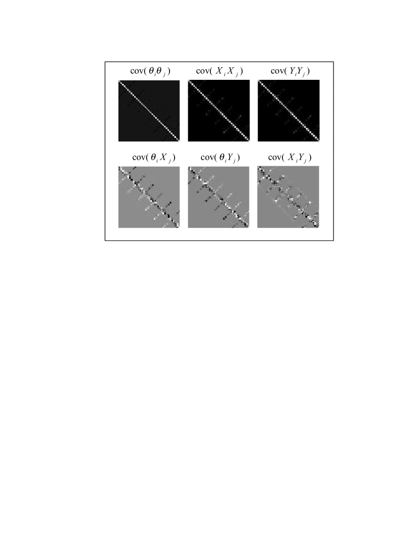
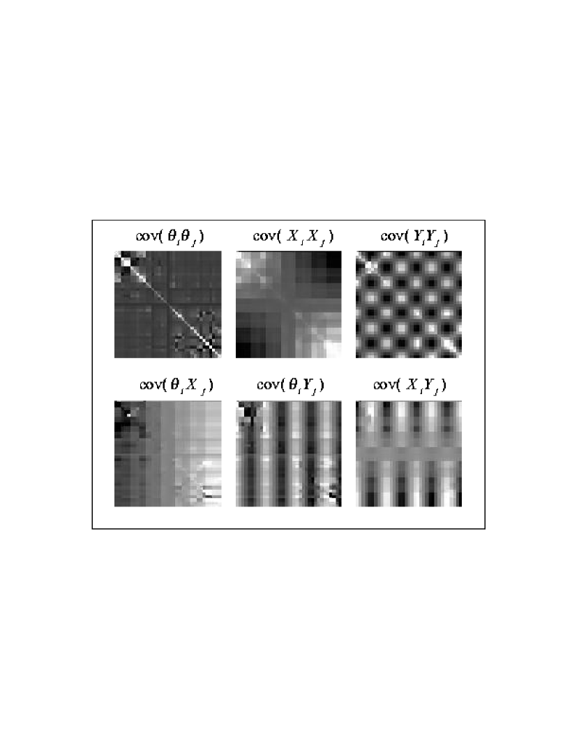
Figure 11 shows greyscale representations of covariance matrices for all combinations of offset parameters (Equation B1) for the 105-image IRAC test case assuming both relative and absolute astrometric source matches in the refinement. With 105 images, each covariance matrix has $105\times 105$ elements (or pixels in this representation). It is important to note that the cross-correlation between different offset types is not symmetric. For instance, the correlation between $\theta_{i}$ and $X_{j}$ is not the same as $\theta_{j}$ and $X_{i}$. Figure 12 shows the same set but with only relative (frame-to-frame) matches used for the refinement. Comparing Figures 11 and 12, we draw the following conclusions: first, for the case including astrometric matches, “long-distance” correlations in image offsets are greatly reduced. This is due to astrometric sources anchoring each image to the fiducial reference frame, making them more independent of each other. The covariance matrices become essentially block-diagonal. Second, uncertainties (variances along the diagonal for the same offset pair combination) are greatly attenuated when astrometric matches are used compared to the relative-only match case. There are greater numbers of degrees of freedom per image when astrometrics are included, and this reduces the relative uncertainty.

The relative-only case exhibits greater long-distance correlations (larger off-diagonal values) since image positions are dictated solely by frame-to-frame matches in image overlap regions. This makes each successive image position dependent on it’s nearest neighbor positions, which depend on their own neighbours and so on throughout the system of linked images. Apart from astrometric matches reducing long distance correlations, this can also happen if prior image pointing uncertainties are intrinsically smaller. Small priors will pull refinement offsets from the global minimization towards zero, which minimizes the $L_{apriori}$ term in Equation 4. The priors force a constraint on each individual image to prevent “over-refinement”, regardless of the number of source matches present. Each image therefore becomes more independent of its neighbors, and long-distance correlations are reduced.

We also note the rich and diverse patterns in the covariance matrices for this observation, especially the relative-only case (Figure 12). These are characteristic of the image layout and mosaic map geometry (see Figure 8). For instance, take the $cov(Y_{i},Y_{j})$ matrix in Figure 12. The checker-board pattern arises from the relative image numbering in the map and how this translates to the numbering of elements in the covariance matrix (Equation B2). In the mosaic, the images repeat from right to left to create a leg, then left to right and down again, for a total of seven legs. Adjacent image pairs ($i,\>j$) along vertical sections in the map are strongly correlated in their ($Y_{i},\>Y_{j}$) offsets, while widely separated images are less correlated. For instance, image number one at top right has its $Y$ offset strongly correlated with the $Y$ offsets of images directly below it (i.e., image numbers 30, 31, 60, 61, 90 and 91). The high correlations are therefore with every $\sim$30th image giving bright regions in the greyscale covariance image. Also, the $Y$ offset of image number one is least correlated with that of images in the far left vertical strip (image numbers 15, 16, 45, 46, 75, 76 and 105), resulting in dark regions in the covariance image.

In the end, one purpose of the covariance matrix is to visualize the degree of correlation between image positions in the ensemble as a whole. This allows one to ascertain whether refinement solutions are driven by any particular invalid input assumptions (e.g., priors), or insufficient astrometric reference source information if robust absolute refinement is desired.

Figure 1: Processing and algorithmic flow in pointingrefine software.

Figure 2: A simple three-image mosaic. Filled circles are sources detected in image n and open circles are sources in m or 1.

Figure 3: One-dimensional representation of projection geometry showing images on sky and in tangent plane of reference image. Images 1 and 2 have the same physical size but different projected sizes.

Figure 4: Unrefined mosaic section of 1000-image IRAC simulation at $3.6\micron$ on left and same section after pointing refinement on right. Field dimensions are $\simeq 2.8\arcmin\times 3.8\arcmin$.

Figure 5: Top: distributions of image center separations relative to “truth” before and after refinement. Bottom: Offsets in RA and Dec between image centers relative to truth. Circle represents 2-$\sigma$ region of truth - refined distribution for case with $\sim 2$ relative/3 absolute matches per image (dot-filled histogram in top figure).

Figure 6: Top: distributions of the magnitude of refinement, represented as a percentage of initial truth - unrefined image separation. Bottom: distributions of matched source radial separations before and after refinement.

Figure 7: Top: uncertainty in matched source radial separation (from centroid uncertainties) as a function of actual source separation after refinement. Bottom: reduced $\chi^{2}$ (i.e., $\chi^{2}$/number of degrees of freedom) as a function of mosaic subset composed of successively increasing numbers of images i (see Section 3).

Figure 8: Coverage mosaic and mapping geometry of the 105-image IRAC observation used in this analysis. Adjacent images have $\sim 20\%$ overlap with a coverage of 6 and 12 pixels at edges and (inner) corners respectively. Mapping direction is shown by arrows starting at top right and ending at bottom left. Open circles are image centers.

Figure 9: Distributions of matched source radial separations before and after refinement for all bands of Spitzer’s IRAC instrument. Relative and absolute astrometric (with 2MASS magnitudes $K_{s}\leq 15$) matches have been separated.

Figure 10: Top: uncertainty in matched source radial separation (from centroid uncertainties of matches) as a function of actual source separation after refinement for IRAC band-1. Bottom: same as Figure 9 for IRAC band-1 but with astrometric matches having a 2MASS magnitude limit of $K_{s}=10$.

Figure 11: Greyscale representation of covariance matrices for all orthogonal and rotational offsets in IRAC test case when absolute astrometric matches are used. See Equation B2 for matrix definition.

Figure 12: Greyscale representation of covariance matrices for all orthogonal and rotational offsets in IRAC test case when absolute astrometric matches are not used (i.e. only relative frame-to-frame matches used). See Equation B2 for matrix definition.

Processing and algorithmic flow in pointingrefine software.

A simple three-image mosaic. Filled circles are sources detected from image n and open circles are sources from m or 1.

One-dimensional representation of projection geometry showing images on sky and in tangent plane of reference image. Images 1 and 2 have the same physical size but different projectedsizes.

Unrefined mosaic section of 1000-image IRAC simulation at $3.6\micron$ on left and same section after pointing refinement on right. Field dimensions are $\simeq 2.8\arcmin\times 3.8\arcmin$.

Top: distributions of image center separations relative to “truth” before and after refinement. Bottom: Offsets in RA and Dec between image centers relative to truth. Circle represents 2-$\sigma$ region of truth - refined distribution for case with $\sim 2$ relative/3 absolute matches per image (dot-filled histogram in top figure).

Top: distributions of the magnitude of refinement, represented as a percentage of initial truth - unrefined image separation. Bottom: distributions of matched source radial separations before and after refinement.

Top: uncertainty in matched source radial separation (from centroid uncertainties) as a function of actual source separation after refinement. Bottom: reduced $\chi^{2}$ (i.e., $\chi^{2}$/number of degrees of freedom) as a function of mosaic subset composed of successively increasing numbers of images i (see Section 3).

Coverage mosaic and mapping geometry of the 105-image IRAC observation used in this analysis. Adjacent images have $\sim 20\%$ overlap with a coverage of 6 and 12 pixels at edges and (inner) corners respectively. Mapping direction is shown by arrows starting at top right and ending at bottom left. Open circles are image centers.

Distributions of matched source radial separations before and after refinement for all bands of Spitzer’s IRAC instrument. Relative and absolute astrometric (with 2MASS magnitudes $K_{s}\leq 15$) matches have been separated.

Top: uncertainty in matched source radial separation (from centroid uncertainties of matches) as a function of actual source separation after refinement for IRAC band-1. Bottom: same as Figure 9 for IRAC band-1 but with astrometric matches having a 2MASS magnitude limit of $K_{s}=10$.

Greyscale representation of covariance matrices for all orthogonal and rotational offsets in IRAC test case when absolute astrometric matches are used. See Equation B2 for matrix definition.

Greyscale representation of covariance matrices for all orthogonal and rotational offsets in IRAC test case when absolute astrometric matches are not used (i.e. only relative frame-to-frame matches used). See Equation B2 for matrix definition.

Table 1: Statistics for IRAC-observation case study.

$\lambda$-Band	$\langle\#Abs.\rangle$	$\langle\#Rel.\rangle$	$\langle D_{bef}\rangle_{A}$	$\langle D_{bef}\rangle_{R}$	$\langle D_{aft}\rangle_{T}$	$\chi^{2}$	dof	$\chi^{2}/$dof
µm			arcsec	arcsec	arcsec
$3.6$	34.7	20.5	0.847	0.605	0.151	8580.84	10821	0.792
$4.5$	20.7	13.7	0.883	0.622	0.152	3843.93	5645	0.681
$5.8$	9.4	7.6	0.933	0.603	0.142	1250.31	2443	0.511
$8.0$	5.3	2.1	0.913	0.651	0.203	1240.50	1249	0.993

References

- Barmby and Lacy (2004) Barmby, P., and Lacy, M. 2004, in preparation
- Barnea and Silverman (1972) Barnea, D. I., and Silverman, H. F. 1972, IEEE Trans. Comput., C-21, 179
- Bly et al. (2002) Bly, M. J., Chipperfield, A. J., Giaretta, D. L., Graffagnino, V. G. et al. 2002, in ASP Conf. Ser. 281, Astronomical Data Analysis Software and Systems XI, ed. D. A. Bohlender, D. Durand, & T. H. Handley (San Francisco: ASP) 513
- Brown (1992) Brown, L. G. 1992, ACM Computing Surveys, 24, 4, 325
- Bustos and Calderón (2000) Bustos, I. H., and Calderón J. H. 2000, Revista Mexicana de Astronomía y Astrofísica, 39, 303
- Calabretta and Greisen (2002) Calabretta, M. R., and Greisen, E. W. 2002, A&A, 395, 1077
- Davis (1996) Davis, L. E. 1996, in ASP Conf. Ser. 101, Astronomical Data Analysis Software and Systems V, ed. G. H. Jacoby & J. Barnes (San Francisco: ASP) 147.
- Evans et al. (2000) Evans, M., Hastings, N., and Peacock, B. 2000, in Statistical Distributions, 3rd ed. New York: Wiley, 57.
- Fazio (2004) Fazio, G. G. 2004, ApJ, (astro-ph/0405616), in press
- Greisen and Calabretta (2002) Greisen, E. W., and Calabretta, M. R. 2002, A&A, 395, 1061
- Kuglin and Hines (1975) Kuglin, C. D., and Hines, D. C. 1975, Proc. IEEE Int. Conf. Cybernet Society, New York, 163
- Lonsdale et al. (2003) Lonsdale, C. J., Smith, H. E., Rowan-Robinson, M., Surace, J. et al. 2003, PASP, 115, 897
- Press et al. (1999) Press, W. H., Teukolsky, S. A., Vetterling, W. T., Flannery, B. P. 1999, Numerical Recipes in C: the art of scientific computing, 2nd ed. (Cambridge UK: Cambridge University Press)
- Valdes (1998) Valdes, F. G. 1998, in ASP Conf. Ser. 145, Astronomical Data Analysis Software and Systems VII, ed. R. Albrecht, R. N. Hook & H. A. Bushouse (San Francisco: ASP) 53
- Veran and Rigaut (1998) Veran, J.-P., and Rigaut, F. J. 1998, Proc. SPIE 3353, Bonaccini; Robert K. Tyson; eds., 426
- Xu et al. (2003) Xu, C. K., Lonsdale, C. J., Shupe, D. L., Franceschini, A., Martin, C. and Schiminovich, D. 2003, ApJ, 587, 90
- Zacharias et al. (2003) Zacharias, N., McCallon, H. L., Kopan, E., Cutri, R. M. 2003, The International Celestial Reference System: Maintenance and Future Realization , 25th meeting of the IAU, Joint Discussion 16, 22 July 2003, Sydney, Australia