A Short Characteristic Solution for the 2.5D Transfer Equation in the Envelopes of O and B Stars

Abstract

We discuss work toward developing a 2.5D non-LTE radiative transfer code. Our code uses the short characteristic method with modifications to handle realistic 3D wind velocities. We also designed this code for parallel computing facilities by representing the characteristics with an impact parameter vector p. This makes the interpolation in the radiation angles unnecessary and allows for an independent calculation for characterisitcs represented by different p vectors. The effects of the velocity field are allowed for by increasing, as needed, the number of grid points along a short characteristic. This allows us to accurately map the variation of the opacities and emissivities as a function of frequency and spatial coordinates. In the future we plan to use this transfer code with a 2D non-LTE stellar atmosphere program (Georgiev et al. 2004) to self-consistently solve for level populations, the radiation field and temperature structure for stars with winds and without spherical symmetry.

Dept. of Physics and Astronomy, University of Pittsburgh, 3941 O’Hara Str., Pittsburgh, PA 15260, USA

Instituto de Astronomia, Universidad Nacional Autonoma de Mexico (UNAM), Apartado Postal 70-264, Mexico 04510, D. F. MX

1. Introduction

Modeling the circumstellar envelopes of O and B stars is a complex nonlinear problem. The non-LTE level populations, the (magneto-) hydrodynamics, and the radiation field are strongly coupled. Thus, an iterative procedure is needed to achieve a consistent solution. An essential constituent of this procedure is the availability of an accurate and fast radiative transfer code.

Progress in computer technology and the availability of fast numerical methods now allow the development of such codes for detailed study of 2D and 3D envelopes. There are several possible avenues to follow. The most straightforward is to solve the general radiative transfer equation

$$\underline{\bf n}{\bf\nabla}I=-\chi\left[I-S\right]$$ (1)

and calculate the radiative transition rates using the solution. In the above $\underline{\bf n}$ is the direction of the radiation, $I$ is the specific intensity, $\chi$ is the opacity, and $S$ is the source function (functional dependence is not indicated for clarity). Alternatively, one could also use the moment equations, derived from Eq. 1, and solve directly for the moments (Hillier & Miller 1998) which set the transition rates; or use Monte-Carlo simulation to solve the radiative transfer equation and calculate estimators of the transition rates (Lucy 1999). We decided to use the first approach because of its simplicity and since it provides a reasonable compromise between numerical efficiency and flexibility.

A simple iteration between the radiative transfer and the rate equations is not a wise choice for the iterative procedure. This is the so-called “$\Lambda$-iteration” which is notorious for convergence difficulties when the optical depth is large. Convergence is ensured, however, by using the Approximate Lambda Iteration (ALI, see e.g., Rybicki & Hummer 1991; Hubeny 1992) which takes some coupling of the radiation and populations into account by using an invertible Approximate Lambda Operator (ALO). In our 2D code we use the local contribution at every spatial point to construct the ALO because it is easy to calculate and has acceptable convergence characteristics. The actual implementation of the ALI procedure into our full non-LTE model atmosphere will be discussed in Georgiev et al. (2004).

2. Description of the Transfer Code

The optical depth and the formal solution of Eq. 1 at any position, $s$, along a ray are

$$\tau_{\nu}=\int_{0}^{s}\chi ds^{\prime} ~{}~{}{\rm and}~{}~{} I(\tau_{\nu})=I_{BC}\,e^{-\tau_{\nu}}\;+\;\int_{0}^{\tau_{\nu}}S(\tau^{\prime})\,e^{\tau^{\prime}-\tau_{\nu}}\,d\tau^{\prime}\;,$$ (2)

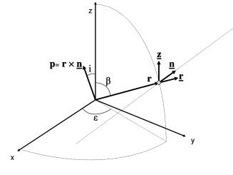
respectively. The intensity can be calculated by specifying I_BC at the up-stream end of the ray (or characterisitic) and by evaluating two integrals. For this purpose, we use the “Short Characteristic” (SC) method, first explored by Mihalas et al. (1978) and Kunasz & Auer (1988). This method requires the evaluation of the integrals only between the point of interest and the closest cell boundary and uses the calculated intensities at other grid points to interpolate $I_{BC}$. In the spherical coordinate system the directional variation of the intensity is normally described by the radiation coordinates $\theta$ and $\phi$, which are defined by

$$cos(\theta)=\underline{\bf n}\cdot\underline{\bf r} ~{}~{}~{}{\rm and}~{}~{}~{} sin(\beta)\cdot sin(\theta)\cdot cos(\phi)=\left[\underline{\bf n}\times\underline{\bf r}\right]\cdot\left[\underline{\bf r}\times\underline{\bf z}\right]\;,$$ (3)

respectively (see Fig. 1 for definitions). Unfortunately, $\theta$ and $\phi$ vary along a characteristic so using the same $\theta$ and $\phi$ grid for all spatial points would require interpolations in these angles. To avoid this additional interpolation we describe a characteristic with

$${\bf p}={\bf r}\times\underline{\bf n}\;,$$ (4)

which we call the “impact parameter vector” (see Fig. 1). This vector describes all essential features of a characteristic and can be considered as an analog of the orbital momentum vector in two body problems. Its absolute value p= $|$p$|$ is the traditional impact parameter while its orientation defines the “orbital plane” of the radiation (the plane that contains the characteristic and the origin). Following the analogy one can define an “inclination” angle for this plane by

$$p\cdot cos(i)={\bf p}\cdot\underline{\bf z}\;.$$ (5)

In our code we set up a universal grid in impact parameters and in inclination angles and calculate the radiation coordinates by

$$sin(\theta)=\frac{p}{r} ~{}~{}~{}{\rm and}~{}~{}~{} sin(\phi)=\frac{cos(i)}{sin(\beta)}$$ (6)

for each grid point (see Fig 1 for definitions).

We evaluate Eq. 2 in the comoving frame of the point of interest which is the proper frame for solving the rate equations. To ensure that the spatial and frequency variations of the opacity and source function are mapped properly in the integrations, we add extra integration points to the characteristics. The number of the extra points (at least one) depends on the ratio of the line of sight velocity difference between the endpoints and a “maximum allowed velocity difference” which is a free parameter in the code. The opacities and source terms at every comoving frequency are then interpoleted onto the integration points by bi-linear approximations using the four closest spatial grid points. It is relatively easy to construct a diagonal ALO in this evaluation scheme.

With the exception of the intensity we interpolate all quantities in first order. However, the accuracy of this approximation is insufficient in many cases; therefore, we introduced a rudimentary multi-grid approach. Before evaluating Eq. 2, we calculate opacity and source function on a dense grid by using a sophisticated 3^rd order approximation. Then, the transfer equation is solved on the original grid using the dense grid for opacity and source term interpolations.

3. Test Results

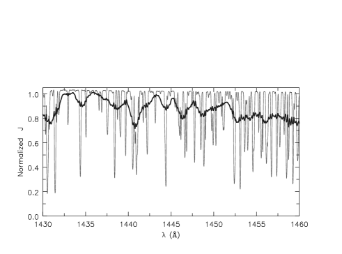
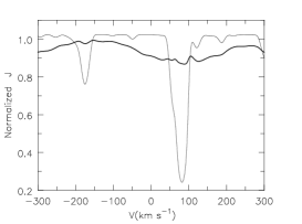
We tested our code by reproducing spherical symmetric CMFGEN models (Hillier & Miller 1998), as well as the results of an accurate 2D long characteristic program (see Busche & Hillier 2000). The 2D models were static with Schuster-type inner boundary conditions and included electron scattering iterations. We were able to reproduce all test cases within $\sim$5% accuracy. In Figs. 2 and 3 we demonstrate the capabilities of our code by showing the results for a rotating stellar envelope. The model was produced by using the opacities and emissivities from the results of a realistic CMFGEN simulation and by introducing a rotational velocity field. As expected the spectral lines show the rotational broadening.

Figure 1.: The definition of our fundamental coordinate system (r, $\beta$, $\epsilon$) and the vectors that are necessary for our notations. Unit vectors $\underline{\bf n}$, $\underline{\bf z}$, and $\underline{\bf r}$ are describing the characteristic (long thin line), the positive z axis, and the radial direction, respectively. The impact parameter vector p and $\underline{\bf n}$ are two alternative ways to define a characteristic.

Figure 2.: The J moment of the radiation field for $\beta$= 0^∘ (thin line) and 45^∘ (thick line) as a function of wavelenght (Å) at the outer boundary of the envelope.

Figure 3.: The spectral region around 1444 Å  from Fig. 2 as a function of velocity (centered on 1444 Å). The rotational velocity in the envelope is $V(r,\beta)=250\cdot r_{*}/r\cdot sin(\beta)$ where $r_{*}$ is the stellar radius.

References

- Busche & Hillier (2000) Busche, J. R. & Hillier, D. J. 2000, ApJ, 531, 1071
- Georgiev et al. (2004) Georgiev L. N., Hillier, D. J., & Zsargó, J. 2004, in preparation
- Hillier & Miller (1998) Hillier, D. J. & Miller, D. L. 1998, ApJ, 496, 407
- Hubeny (1992) Hubeny, I. 1992, in The Atmospheres of Early-Type Stars, ed. U. Heber & C. J. Jeffery (Berlin:Springer), 377
- Kunasz & Auer (1988) Kunasz, P. B., & Auer, L. H. 1988, J. Quant. Spectrosc. Radiat. Transfer, 39, 67
- Lucy (1999) Lucy, L. B. 1999, A&A, 344, 282
- Mihalas et al. (1978) Mihalas, D., Auer, L. H., & Mihalas, B. W. 1978, ApJ, 220, 1001
- Rybicki & Hummer (1991) Rybicki, G. B. & Hummer, D. G. 1991, A&A, 245,171