Molecular hydrogen in damped Ly$\alpha$ systems: clues to interstellar physics at high-redshift

Abstract

In order to interpret H₂ quasar absorption line observations of damped Ly$\alpha$ systems (DLAs) and sub-DLAs, we model their H₂ abundance as a function of dust-to-gas ratio, including H₂ self-shielding and dust extinction against dissociating photons. Then, we constrain the physical state of gas by using H₂ data. Using H₂ excitation data for DLA with H₂ detections, we derive a gas density $1.5\la\log n~{}[{\rm cm}^{-3}]\la 2.5$, temperature $1.5\la\log T~{}[{\rm K}]\la 3$, and internal UV radiation field (in units of the Galactic value) $0.5\la\log\chi\la 1.5$. We then find that the observed relation between molecular fraction and dust-to-gas ratio of the sample is naturally explained by the above conditions. However, it is still possible that H₂ deficient DLAs and sub-DLAs with H₂ fractions less than $\sim 10^{-6}$ are in a more diffuse and warmer state. The efficient photodissociation by the internal UV radiation field explains the extremely small H₂ fraction ($\la 10^{-6}$) observed for $\kappa\la 1/30$ ($\kappa$ is the dust-to-gas ratio in units of the Galactic value); H₂ self-shielding causes a rapid increase and the large variations of H₂ abundance for $\kappa\ga 1/30$. We finally propose an independent method to estimate the star formation rates of DLAs from H₂ abundances; such rates are then critically compared with those derived from other proposed methods. The implications for the contribution of DLAs to the cosmic star formation history are briefly discussed.

1 Introduction

Damped Ly$\alpha$ clouds (DLAs) are quasar (QSO) absorption line systems whose neutral hydrogen column density is larger than $\sim 1-2\times 10^{20}$ cm^-2 (e.g. Prochaska & Wolfe 2002). DLAs absorb Ly$\alpha$ photons at the restframe of the DLAs. Because QSOs are generally luminous, DLAs provide us with unique opportunities to trace high-redshift (high-$z$) galaxy evolution. In particular, by identifying absorption lines of various species, the physical condition of the interstellar medium (ISM) of DLAs has been deduced.

From the analyses of various absorption lines, evidence has been found for the existence of heavy elements in DLAs (e.g. Lu et al. 1996). The evolution of metal abundance in DLAs can trace the chemical enrichment history of present galaxies. Based on this, and on other clues, DLAs have been suggested to be the progenitors of nearby galaxies; the similar values of the baryonic mass density in DLAs around redshift $z\sim 2$ and the stellar mass density at $z\sim 0$ has further supported this idea (Lanzetta, Wolfe, & Turnshek 1995; Storrie-Lombardi & Wolfe 2000). By adopting a recently favoured $\Lambda$CDM cosmology, however, Péroux et al. (2003) argue that the comoving density of H i gas at $z\sim 2$ is smaller than the comoving stellar mass density at $z\sim 0$. Yet they strengthen the importance of DLAs, showing that a large fraction of H i gas is contained in DLAs at $z\sim 2$–3.

In general, a certain fraction of metals condenses onto dust grains. Indeed, Fall, Pei, & McMahon (1989) have suggested that the reddening of background quasars indicates typical dust-to-gas ratios of $\sim 1/20$–1/4 of the Milky Way (see also Zuo et al. 1997, but see Murphy & Liske 2004). The depletion of heavy elements also supports the dust content in DLAs (Pettini et al. 1994; Vladilo 2002). The existence of dust implies the possibility that the formation of hydrogen molecules (H₂) is enhanced because of the H₂ grain surface reaction (Lanzetta, Wolfe, & Turnshek 1989). Hirashita & Ferrara (2002) argue that the enhancement of molecular abundance results in an enhancement of the star formation activity in the early evolutionary stages of galaxy evolution, because stars form in molecular clouds. The important role of dust on the enhancement of the H₂ abundance is also suggested by observations of DLAs (Ge, Bechtold, & Kulkarni 2001; Ledoux, Petitjean, & Srianand 2003) and in the local Universe, e.g. in Galactic (Milky Way) halo clouds (e.g. Richter et al. 2003) and in the Magellanic Clouds (Richter 2000; Tumlinson et al. 2002).

Although the H₂ fraction (the fraction of hydrogen nuclei in the form of H₂; see equation 11) is largely enhanced for some DLAs, stringent upper limits are laid on a significant fraction of DLAs in the range $\la 10^{-7}$–$10^{-5}$ (Black, Chaffee, & Foltz 1987; Petitjean, Srianand, & Ledoux 2000). This can be interpreted as due to a low formation rate of H₂ in dust-poor environments relative to the Milky Way (Levshakov et al. 2002; Liszt 2002) and high H₂ dissociation rate by strong ultraviolet (UV) radiation (e.g. Petitjean et al. 2000). However, we should keep in mind that such upper limits do not exclude the existence of molecule-rich clouds in these systems, because molecular clouds may have a very low volume filling factor. Indeed, based on the hydrodynamical simulation of Wada & Norman (2001), Hirashita et al. (2003) show that under a strong UV field typical of high-$z$ and a poor dust content ($\sim 1/10$ of the Galactic dust-to-gas ratio), H₂-rich regions are located in very clumpy small regions. In such a situation, it is natural that molecular clouds are hardly detected in DLAs.

The probability of detecting H₂ is higher for DLAs with larger dust-to-gas ratio or larger metallicity. Indeed, H₂ tends to be detected for metal-rich DLAs (Ledoux et al. 2003). The correlation between dust-to-gas ratio and H₂ abundance for DLAs indicates that H₂ predominantly forms on dust grains as in the Galaxy (e.g. Jura 1974). Since the H₂ formation and destruction rates are affected mainly by gas density, dust-to-gas ratio, and UV radiation intensity, we can derive or constrain those quantities for DLAs based on H₂ abundance. Those quantities also enable us to draw conclusions about other important quantities such as cooling and heating rates, star formation rate (SFR), etc. (Wolfe, Prochaska, & Gawiser 2003a).

Our main aim in this paper is to investigate what we can learn from the recent H₂ observations of DLAs and sub-DLAs. (Although we mainly focus on DLAs, we also include low column density systems, which are called sub-DLAs.) In particular, we focus on key quantities for H₂ formation and destruction (i.e. dust-to-gas ratio and UV intensity, respectively). The physical state of H₂ reflects the physical state of gas, especially, gas density and temperature. In this work, we concentrate on H₂ data to derive those physical quantities. Recent FUSE (Far Ultraviolet Spectroscopic Explorer) observations of the Galactic ISM (e.g. Gry et al. 2002; Marggraf, Bluhm, & de Boer 2004), the Galactic halo clouds (e.g. Richter et al. 2003), and the Magellanic Clouds (e.g. Tumlinson et al. 2002; Richter, Sembach, & Howk 2003; André et al. 2004) are successful in deriving the physical state of gas from H₂ absorption line data. We focus on DLAs and sub-DLAs to investigate the high-$z$ universe. Since recent observations suggest that the local UV radiation originating from star formation within DLAs is stronger than the UV background intensity (Ledoux, Srianand, & Petitjean 2002; Wolfe et al. 2003a), we include the local UV field in this work. We call the local UV field “interstellar radiation field (ISRF)”.

Since it is still unclear whether DLAs are large protogalactic discs (Wolfe et al. 1986; Prochaska & Wolfe 1998; Salucci & Persic 1999), small sub-$L^{*}$ galaxies (Gardner et al. 2001; Møller et al. 2002; Okoshi et al. 2004), protogalactic clumps (Haehnelt, Steinmetz, & Rauch 1998; Ledoux et al. 1998), or a mixture of various populations (Burbidge et al. 1996; Cen et al. 2003; Rao et al. 2003), we adopt a simple model which nevertheless includes all relevant physical processes and derive robust general conclusions.

We first describe the model we use to derive the molecular content in DLAs (Section 2). After describing the observational sample adopted in this paper (Section 3), we compare our results with the data and constrain the physical conditions of DLAs (Section 4). Based on these results, we extend our discussion to the SFR (Section 5), and we finally give a summary of this paper (Section 6).

2 Model

Our aim is to investigate the physical conditions in the ISM of DLAs by treating H₂ formation and destruction for a statistical sample. For the homogeneity of our analysis, we concentrate our interest on H₂. Our aim is not to analyse the data of each object in detail by using various absorption lines of various species, since different lines may originate from different places and detected lines are different from object to object. Our model is analytical for the simple application to a large statistical sample. There are a lot of works that treat details of various gas state by fitting the observational results of absorption lines of various atoms and molecules. Therefore, our model may be too simple to derive a precise physical quantities for each object. However, our analysis has the following advantages for the statistical purpose: (i) A large sample is treated homogeneously, since we concentrate only on H₂ in an analytic way. (ii) The results directly conclude the statistical properties of DLAs and are not affected by details and peculiar situations of each object.

The relevant physical quantities are those concerning the H₂ formation and destruction, that is, molecular fraction, dust-to-gas ratio, UV radiation field, and gas density and temperature. Observationally, the molecular fraction, the dust-to-gas ratio and the H i column density are relatively well known, but the UV radiation field, and the gas density and temperature are poorly constrained. Thus, we first constrain the reliable ranges in those quantities by reviewing H₂ detected objects. Then, the likelihood of those parameters are discussed by using a statistical sample.

2.1 H₂ formation and destruction

For the metallicity range typical of DLAs, we can assume equilibrium between H₂ formation and destruction, because the timescale of H₂ formation and destruction is well below the dynamical timescale (Hirashita et al. 2003). We adopt the formation rate of H₂ per unit volume and time, $R_{\rm dust}$, by Hollenbach & McKee (1979) (see also Hirashita et al. 2002):

$$R_{\rm dust} = 4.1\times 10^{-17}S_{\rm d}(T)\left(\frac{a}{0.1~{}\mu{\rm m}}\right)^{-1}\left(\frac{{\cal D}}{10^{-2}}\right)$$ (1)

$$\times \left(\frac{T}{100~{}{\rm K}}\right)^{1/2}\left(\frac{\delta}{2~{}{\rm g}~{}{\rm cm}^{-3}}\right)~{}{\rm cm^{3}~{}s^{-1}}\,,$$

where $a$ is the radius of a grain (assumed to be spherical with a radius of 0.1 $\mu$m unless otherwise stated), ${\cal D}$ is the dust-to-gas mass ratio (varied in this paper; the typical value in the solar vicinity of the Milky Way is $10^{-2}$), $\delta$ is the grain material density (assumed to be 2 g cm^-3 in this paper), and $S_{\rm d}(T)$ is the sticking coefficient of hydrogen atoms onto dust. The sticking coefficient is given by (Hollenbach & McKee 1979; Omukai 2000)

$$S_{\rm d}(T) = [1+0.04(T+T_{\rm d})^{0.5}+2\times 10^{-3}T+8\times 10^{-6}T^{2}]^{-1}$$ (2)

$$\times [1+\exp(7.5\times 10^{2}(1/75-1/T_{\rm d}))]^{-1}\,,$$

where $T_{\rm d}$ is the dust temperature, which is calculated by assuming the radiative equilibrium in equation (12). However, since the reaction rate is insensitive to the dust temperature as long as $T_{\rm d}\la 70$ K, the following results are not affected by the dust temperature. In fact, $T_{\rm d}$ never exceeds 70 K under the radiation field intensity derived in this paper. The H₂ formation rate per unit volume is estimated by $R_{\rm dust}nn_{\rm H}$, where $n$ is the gas number density, and $n_{\rm H}$ is the number density of H i.

The H₂ formation rate on dust grains is still to be debated. It depends on grain size (eq. 1). If the grain size is much smaller than 0.1 $\mu$m, the H₂ formation rate is largely enhanced. There are uncertainties also in $S_{\rm d}(T)$, which could depend on the materials of dust. Cazaux & Tielens (2002) also suggest that $S_{\rm d}(T)$ in equation (1) should be substituted by $\epsilon_{\rm H_{2}}S_{\rm d}(T)$, where $\epsilon_{\rm H_{2}}$ is the recombination efficiency (the fraction of the accreted hydrogen that desorbs as H₂). The recombination efficiency is $\epsilon_{\rm H_{2}}\sim 1$ if $5\la T\la 30$ K, and $\epsilon_{\rm H_{2}}$ becomes $\sim 0.2$ at $T\sim 100$ K. If the temperature is higher than $\sim 300$ K, $\epsilon_{\rm H_{2}}\sim 0$. However, if $\epsilon_{\rm H_{2}}\sim 0.2$ is multiplied to the H₂ formation rate at $T=100$ K, the grain formation rate becomes significantly small, and the Galactic H₂ formation rate derived for $T\sim 100$ K by Jura (1974) cannot be achieved; we have to keep in mind that the theoretical determination of $R_{\rm dust}$ is affected by some uncertainty. Thus, in this paper, we adopt equation (1) to assure that it provides the Galactic H₂ formation rate if we adopt $a\sim 0.1~{}\mu$m, ${\cal D}\sim 0.01$, $T\sim 100$ K, and $\delta\sim 2$ g cm^-3. Since it is important to recongnise that the temperature dependence of $R_{\rm dust}$ is uncertain, we do not deeply enter discussions on the temperature dependence in this paper.

The photodissociation rate $R_{\rm diss}$ is estimated as (Abel et al. 1997)

$$R_{\rm diss}=(4\pi)\,1.1\times 10^{8}J_{\rm LW}\,S_{\rm shield}~{}{\rm s}^{-1}\,,$$ (3)

where $J_{\rm LW}$ (erg s^-1 cm^-2 Hz^-1 sr^-1) is the UV intensity at $h\nu=12.87$ eV averaged over the solid angle, $S_{\rm shield}$ is the correction factor of the reaction rate for H₂ self-shielding and dust extinction. The photodissociation rate per unit volume is estimated as $R_{\rm diss}n_{\rm H_{2}}$, where $n_{\rm H_{2}}$ is the number density of H₂. We adopt the correction for the H₂ self-shielding by Draine & Bertoldi (1996) (see also Hirashita & Ferrara 2002). Then, we estimate $S_{\rm shield}$ as

$$S_{\rm shield}={\rm min}\left[1,\,\left(\frac{N_{\rm H_{2}}}{10^{14}~{}{\rm cm}^{-2}}\right)^{-0.75}\right]e^{-\sigma_{\rm d}N_{\rm d}}\,,$$ (4)

where $N_{\rm H_{2}}$ and $N_{\rm d}$ are the column densities of H₂ and dust, respectively, and $\sigma_{\rm d}$ is the cross section of a grain against H₂ dissociating photons. In the UV band, $\sigma_{\rm d}$ is approximately estimated with the geometrical cross section: $\sigma_{\rm d}\simeq\pi a^{2}$ (Draine & Lee 1984). The column density of grains is related to $N_{\rm H}$: $(4/3)\pi a^{3}\delta N_{\rm d}=1.4m_{\rm H}N_{\rm H}{\cal D}$ (the factor 1.4 is the correction for the helium content). Therefore, the optical depth of dust in UV, $\tau_{\rm UV}\equiv\sigma_{\rm d}N_{\rm d}$, is expressed as

$$\tau_{\rm UV} = \frac{4.2N_{\rm H}m_{\rm H}{\cal D}}{4a\delta}$$ (5)

$$= 0.879\left(\frac{a}{0.1~{}\mu{\rm m}}\right)^{-1}\left(\frac{\delta}{2~{}{\rm g~{}cm}^{-3}}\right)^{-1}\left(\frac{{\cal D}}{10^{-2}}\right)$$

$${}\times\left(\frac{N_{\rm H}}{10^{21}~{}{\rm cm}^{-2}}\right)\,.$$

Since ${\cal D}<10^{-2}$ for DLAs (often ${\cal D}\ll 10^{-2}$), the dust extinction is negligible except for the high column density and dust-rich regime satisfying $N_{\rm H}{\cal D}\ga 10^{19}~{}{\rm cm}^{-2}$. We also define the critical molecular fraction, $f_{\rm H_{2}}^{\rm cr}$ as the molecular fraction which yields $N_{\rm H_{2}}=10^{14}$ cm^-2:

$$f_{\rm H_{2}}^{\rm cr}(N_{\rm H})\equiv 2\times 10^{14}/N_{\rm H}\,.$$ (6)

For $f_{\rm H_{2}}>f_{\rm H_{2}}^{\rm cr}$, the self-shielding affects the H₂ formation.

In this paper, we assume the Galactic (Milky Way) dust-to-gas ratio to be ${\cal D}_{\odot}=0.01$. We define the normalised dust-to-gas ratio $\kappa$ as

$$\kappa\equiv{\cal D}/{\cal D}_{\odot}\,.$$ (7)

The typical Galactic ISRF intensity has been estimated to be $c\nu u_{\nu}=1.2\times 10^{-3}$ erg cm^-2 s^-1 at the wavelength of 1000 Å (i.e. $\nu=3.0\times 10^{15}$ Hz), where $u_{\nu}$ is the radiation energy density per unit frequency (Habing 1968). Approximating the energy density of photons at 1000 Å with that at the Lyman-Werner Band, we obtain for $J_{\rm LW}$ at the solar vicinity, $J_{\rm LW\odot}\simeq cu_{\nu}/4\pi=3.2\times 10^{-20}$ erg s ^-1 cm^-2 Hz^-1 sr^-1. The intensity normalised to the Galactic ISRF, $\chi$, is defined by

$$\chi\equiv J_{\rm LW}/J_{\rm LW\odot}\,.$$ (8)

Using equations (3) and (8), we obtain

$$R_{\rm diss}=4.4\times 10^{-11}\chi S_{\rm shield}~{}{\rm s}^{-1}\,.$$ (9)

With $\chi=1$, the formula reproduces the typical Galactic photodissociation rate (2–$5\times 10^{-11}~{}{\rm s}^{-1}$) derived by Jura (1974).

The UV background intensity at the Lyman limit is estimated to be $J_{21}=0.3$–1 around $z\sim 3$, where $J_{\rm 21}$ is in units of $10^{-21}$ erg cm^-2 s^-1 Hz^-1 sr^-1 (Haardt & Madau 1996; Giallongo et al. 1996; Cooke, Espey, & Carswell 1997; Scott et al. 2000; Bianchi, Cristiani, & Kim 2001). If we assume that the Lyman limit intensity is equal to the Lyman-Werner luminosity, we roughly obtain $\chi=32J_{\rm 21}$. The UV background intensity is likely to be lower at $z\la 1$ (e.g. Scott et al. 2002). Thus, the internal stellar radiation is dominant for H₂ dissociation if $\chi\ga 1/32$.

As mentioned at the beginning of this subsection, we can assume that the formation and destruction of H₂ are in equilibrium. Therefore, the following equation holds:

$$R_{\rm dust}nn_{\rm H}=R_{\rm diss}n_{\rm H_{2}}\,.$$ (10)

In order to solve this equation, it is necessary to give the gas temperature $T$, the gas number density $n$, the normalised dust-to-gas ratio $\kappa$, the normalised ISRF $\chi$, and the column density $N_{\rm H}$. As for the dust grains, we assume $a=0.1~{}\mu$m, and $\delta=2~{}{\rm g}~{}{\rm cm}^{-3}$, all of which are typical values in the local universe. After solving that equation, the molecular fraction is obtained from the definition:

$$f_{\rm H_{2}}\equiv\frac{2n_{\rm H_{2}}}{n_{\rm H}+2n_{\rm H_{2}}}\,,$$ (11)

where we neglect the ionised hydrogen for DLAs.

2.2 Dust temperature

Dust temperature is necessary to calculate the sticking efficiency of H onto grains (equation 2). The equilibrium dust temperature is determined from the balance between incident radiative energy and radiative cooling. We adopt the equilibrium temperature calculated by Hirashita & Hunt (2004) (see also Takeuchi et al. 2003):

$$T_{\rm d} = 12\,(\chi Q_{\rm UV})^{1/6}\left(\frac{A}{3.2\times 10^{-3}~{}{\rm cm}}\right)^{-1/6}$$ (12)

$${}\times\left(\frac{a}{0.1~{}\mu{\rm m}}\right)^{-1/6}~{}{\rm K}\,,$$

where the constant $A$ depends on the optical properties of dust grains, and for silicate grains $A=1.34\times 10^{-3}$ cm (Drapatz & Michel 1977), while for carbonaceous grains $A=3.20\times 10^{-3}$ cm (Draine & Lee 1984; Takeuchi et al. 2003). We hereafter assume $Q_{\rm UV}=1$, $A=3.20\times 10^{-3}$ cm, and $a=0.1~{}\mu$m; these assumptions affect very weakly our calculations due to the 1/6 power index dependence of those parameters.

2.3 Approximate scaling of molecular fraction

As a summary of our formulation, we derive an approximate scaling relation for $f_{\rm H_{2}}$. The molecular fraction is determined from equation (10). The left-hand side describes the formation rate, which follows the scaling relation, $R_{\rm dust}\propto\kappa T^{1/2}S_{\rm d}(T)$. On the other hand, the H₂ destruction coefficient $R_{\rm diss}$ is proportional to $\chi$ for $f_{\rm H_{2}}N_{\rm H}<10^{14}~{}{\rm cm}^{-2}$ (unshielded regime), and is proportional to $\chi(f_{\rm H_{2}}N_{\rm H})^{-0.75}$ for $f_{\rm H_{2}}N_{\rm H}>10^{14}~{}{\rm cm}^{-2}$ (shielded regime). As mentioned in Section 2.1, the self-shielding is more important than the dust extinction. Thus, we neglect the dust extinction in this subsection.

Under the condition that $n_{\rm H_{2}}\ll n_{\rm H}$, $f_{\rm H_{2}}\simeq 2n_{\rm H_{2}}/n_{\rm H}\ll 1$, and by using the expressions above for $R_{\rm dust}$ and $R_{\rm diss}$, we obtain the following scaling relations for $f_{\rm H_{2}}$ from equation (10): in the unshielded regime ($f_{\rm H_{2}}N_{\rm H}<10^{14}~{}{\rm cm}^{-2}$),

$$f_{\rm H_{2}}\propto\kappa n\chi^{-1}T^{1/2}S_{\rm d}(T)\,,$$ (13)

and in the shielded regime ($f_{\rm H_{2}}N_{\rm H}>10^{14}~{}{\rm cm}^{-2}$),

$$f_{\rm H_{2}}\propto[\kappa n\chi^{-1}T^{1/2}S_{\rm d}(T)]^{4}N_{\rm H}^{3}\,.$$ (14)

We have adopted the approximate formula $S_{\rm shield}\propto N_{\rm H_{2}}^{-0.75}$ for $N_{\rm H_{2}}>10^{14}~{}{\rm cm}^{-2}$. In fact, there is a slight (factor of $\sim 2$) difference between this scaling and the exact calculation (Figs. 3–5 of Draine & Bertoldi 1996). In the self-shielding regime, this slight difference may cause an order of magnitude difference in the calculated $f_{\rm H_{2}}$ because of a nonlinear dependence on $N_{\rm H_{2}}$ (see the appendix of Abel et al. 2004). In practice, this difference can also be examined by changing $R_{\rm dust}$ in stead of $R_{\rm diss}$, and indeed, if we change $R_{\rm dust}$ by a factor of $\sim 3$, the calculated molecular fraction is significantly affected as shown in Section 4. For the statistical purpose, however, our conclusions are robust, since $N_{\rm H_{2}}$ spans over a wide range in our sample and the fitting formula approximate the overall trend of $S_{\rm shield}$ as a function of $N_{\rm H_{2}}$ very well.

3 DATA SAMPLE

3.1 Overview

Recently, Ledoux et al. (2003) have compiled a sample of Ly$\alpha$ clouds with H₂ observations. The H i column density of their sample ranges from $\log N(\mbox{H {\sc i}})=19.35$ to 21.70. They have found no correlation between $\log N(\mbox{H {\sc i}})$ and $\log f_{\rm H_{2}}$, but have found clear correlation between the metal depletion (or dust-to-gas ratio, $\log\kappa$) and $\log f_{\rm H_{2}}$. Although some clouds have H i column densities smaller than the threshold for DLAs (typically $\log N(\mbox{H {\sc i}})\ga 20.3$), we treat all the sample, because there is no physical reason for using this threshold for H i. Such low-column density objects called sub-DLAs can be useful to investigate a wider range of $N(\mbox{H {\sc i}})$ and get an an insight into several physical processes, especially self-shielding. For the absorption system of Q 0013$-$004 (the absorption redshift is $z_{\rm abs}=1.973$), we adopt the mean of the two values, $-1.73$, for $\log f_{\rm H_{2}}$ (but in the figures, the observationally permitted range, $-2.81<\log f_{\rm H_{2}}<-0.64$, is shown by a bar). Since it is likely that almost all the hydrogen nuclei are in the form of H i, we use $N(\mbox{H {\sc i}})$ and $N_{\rm H}$ interchangeably. (If the ionised hydrogen is not negligible in a system, we can interpret our result to be representative of the neutral component in the system.)

Ledoux et al. (2003) observationally estimate the dust-to-gas ratio $\kappa$ from the metal depletion:

$$\kappa=10^{[{\rm X/H}]}(1-10^{[{\rm Fe/X}]})\,,$$ (15)

where X represents a reference element that is little affected by dust depletion effects. We adopt this formula in this paper. A formal derivation of equation (15) is given by Wolfe et al. (2003a). Ledoux et al. (2003) have shown a correlation between $\log\kappa$ and $\log f_{\rm H_{2}}$, which strongly suggests that H₂ forms on dust grains. Stringent upper limits are laid on DLAs with $\log\kappa\la-1.5$. It should also be noted that for DLAs with $\log\kappa\ga-1.5$ there is a large dispersion in $\log f_{\rm H_{2}}$. This dispersion implies that the molecular abundance is not determined solely by the dust-to-gas ratio. Therefore, it is necessary to model the statistical dispersion of $\log f_{\rm H_{2}}$.

In Figure 1, we plot the relation between molecular fraction and dust-to-gas ratio of Ledoux et al. (2003) (see their paper for details and error bars). We also plot the data of a Ly$\alpha$ absorber in which H₂ is detected (the absorption redshift, $z_{\rm abs}=1.15$) toward the QSO HE 0515$-$4414 (Reimers et al. 2003). For this absorber, we adopt $\log N(\mbox{H {\sc i}})=19.88$, $\log f_{\rm H_{2}}=-2.64$, and $\log\kappa=-0.051$ (Reimers et al. 2003). The lines in those figures are our model predictions, which are explained in the following section.

Figure 1: Relation between $f_{\rm H_{2}}$ (the molecular fraction of hydrogen) and $\kappa$ (dust-to-gas ratio normalised by the Galactic value). The squares are the observational data compiled by Ledoux et al. (2003). The data with upward and downward arrows indicate that only lower and upper limits for $f_{\rm H_{2}}$ are obtained, respectively, and those with rightward and leftward arrows show lower and upper limits for $\kappa$, respectively. The cross is the data of Reimers et al. (2003). The thick solid, dotted, dashed, dot-dashed lines present our calculations for $n=100~{}{\rm cm}^{-3}$, $T=100$ K, and $\chi=10$ with different H i column densities ($10^{21}$, $10^{19}$, $10^{20}$, and $10^{22}$ cm^-2, respectively). The thin solid line represents the calculation with the same parameters as the thick solid line except for a high formation rate of $R_{\rm dust}$ (small grains with $a=0.03~{}\mu$m is assumed and $R_{\rm dust}$ becomes 3.3 times larger).

We also use the H i column density. In particular, Ledoux et al. (2003) show that there is no evidence of correlation between H i column density and molecular fraction.

3.2 Individual H₂-detected objects

In order to derive the reasonable range of physical quantities characterising Ly$\alpha$ absorbers, we use the H₂ data. The objects whose H₂ absorption lines are detected allow us to constrain the physical state of gas. As mentioned in Section 2, our analysis is limited to H₂. The excitation temperature is related to the ratio of the column densities as (e.g. Levshakov et al. 2000):

$$\frac{N(J)}{N(0)}=\frac{g_{J}}{g_{0}}\exp\left[-\frac{B_{v}J(J+1)}{T_{J0}}\right]\,,$$ (16)

where $N(J^{\prime})$ is the column density of H₂ in the level $J=J^{\prime}$, the statistical weight of a level $J$, $g_{J}$, is $3(2J+1)$ for odd $J$ and $(2J+1)$ for even $J$, and the constant $B_{v}=85.36$ K is applicable to the vibrational ground state. If the column densities of H₂ in the rotational $J$-th and ground states are known, we can determine the excitation temperature $T_{J0}$ by solving the above equation. In particular, $T_{10}$ is the best tracer for the kinetic temperature (Jura 1975). Therefore, we approximate $T\sim T_{10}$ in the discussion of this section.

Using the column densities of $J=4$ or 5 level, we can constrain the gas density following the simple procedure introduced by Jura (1975). Those levels are populated by direct formation into these levels of newly created molecules, and by pumping from $J=0$ and $J=1$. The assumption that the lowest two levels ($J=0$ and 1) are dominated in population holds also to the H₂ detected DLAs. Following Jura (1975) we adopt $\beta(0)\simeq\beta(1)$ (see also Jura 1974), where $\beta(J)$ is the total rate of an upward radiative transition from level $J$ by absorbing Lyman- and Werner-band photons. This assumption is true as long as the saturation levels of absorption are the same. The distribution function of the levels of formed H₂ is taken from Spitzer & Zweibel (1974), who treat a typical interstellar condition. We use the ratio of two column densities at the levels $J=1$ and $J=0$, $N(1)/N(0)$, and assume that $f_{1,0}\equiv n_{\rm H_{2}}(1)/n_{\rm H_{2}}(0)=N(1)/N(0)$, where $n_{\rm H_{2}}(J^{\prime})$ is the hydrogen number density in the level $J=J^{\prime}$. Then we can rewrite equations (3a) and (3b) of Jura (1975) in the following forms:

$$A(4\to 2)\frac{n_{\rm H_{2}}(4)}{n_{\rm H}}=R_{\rm dust}n\left(0.19+\frac{9.1}{1+f_{1,0}}p_{4,0}\right)\,,$$ (17)

$$A(5\to 3)\frac{n_{\rm H_{2}}(5)}{n_{\rm H}}=R_{\rm dust}n\left(0.44+\frac{9.1f_{1,0}}{1+f_{1,0}}p_{5,1}\right)\,,$$ (18)

where $p_{4,0}$ and $p_{5,1}$ are the pumping efficiencies into the $J=4$ and $J=5$ levels from the $J=0$ and $J=1$ levels, respectively, and $A(J^{\prime}\to J^{\prime\prime})$ denotes the spontaneous transition probability from $J=J^{\prime}$ to $J=J^{\prime\prime}$. The H₂ formation rate coefficient $R_{\rm dust}$, the gas particle number density $n$, and the number density of H i $n_{\rm H}$ are defined in Section 2.1. We adopt $A(4\to 2)=2.76\times 10^{-9}~{}{\rm s}^{-1}$, $A(5\to 3)=9.85\times 10^{-9}~{}{\rm s}^{-1}$ (Spitzer 1978), $p_{4,0}=0.26$, and $p_{5,1}=0.12$ (Jura 1975).

Assuming $n_{\rm H_{2}}(4)/n_{\rm H}=N(4)/N_{\rm H}$ and $n_{\rm H_{2}}(5)/n_{\rm H}=N(5)/N_{\rm H}$, we estimate the gas number density $n$ from equations (17) and/or (18). $R_{\rm dust}$ is given by equation (1), where we adopt the observational dust-to-gas ratio for $\kappa$ and the excitation temperature $T_{10}$ for $T$. Here we assume that $T_{\rm dust}=12$ K, because we do not know the ISRF at this stage. However, this assumption does not affect the result in the range of $T_{\rm dust}$ consistent with the range of $\chi$ estimated below.

Finally equation (10) is used to obtain the UV radiation field $\chi$ (proportional to $R_{\rm diss}$; equation 9, where $S_{\rm shield}$ depends on $N_{\rm H_{2}}$) by using the estimated $T=T_{10}$ and $n$, and the observed value of $n_{\rm H_{2}}/n_{\rm H}=N_{\rm H_{2}}/N_{\rm H}$. Each H₂-detected object is discussed separately in the following. This simple analytical method suffices for the statistical character of our study. Careful treatments focusing on individual objects may require a more detailed treatment of H₂ excitation state as described, for example, in Browning, Tumlinson, & Shull (2003).

3.2.1 Q 0013$-$004 ($z_{\rm abs}=1.968$)

The excitation temperature is estimated to be $T_{10}=73$ K (Petitjean, Srianand, & Ledoux 2002). Only the upper limit is obtained for $N_{\rm H}$ ($\log N_{\rm H}~{}[{\rm cm}^{-2}]\leq 19.43$). Thus, $N(4)/N_{\rm H}\geq 3.2\times 10^{-5}$ and $N(5)/N_{\rm H}\geq 1.3\times 10^{-5}$. Those two values indicate $R_{\rm dust}n\geq 6.0\times 10^{-14}~{}{\rm s}^{-1}$ and $R_{\rm dust}n\geq 1.4\times 10^{-13}~{}{\rm s}^{-1}$, respectively. This formation rate is very high compared with the Galactic molecular clouds (e.g. Jura 1975), and if the Galactic dust-to-gas ratio is assumed, we obtain $n>6\times 10^{3}$ cm^-3. However, with this high density, the levels $J=2$ should be in thermal equilibrium, but $T_{20}=302$ K, which is higher than $T_{10}$. This indicates that the gas density should be less than the critical density, $n\la 200~{}{\rm cm}^{-3}$, which is consistent with the density derived from C i lines (10–85 cm^-3; Petitjean et al. 2002). The discrepancy between a density derived from H₂ and one from C i is also reported for the absorption system of HE 0515$-$4414 (Reimers et al. 2003; Section 3.2.9). They suspect that the H₂ formation rate is larger than the Galactic value. For example, if the grain size is typically smaller than that assumed in equation (1), the formation rate becomes larger.

Since only the lower limits are obtained for $N_{\rm H_{2}}/N_{\rm H}$ and $R_{\rm dust}n$, it is not possible to determine $\chi$. By using $\log N_{\rm H_{2}}=16.77$, we obtain $S_{\rm shield}=8.4\times 10^{-3}$. It may be reasonable to assume that $N_{\rm H}/N_{\rm H_{2}}\ga 1$, and in this case, we obtain $R_{\rm diss}=R_{\rm dust}n(N_{\rm H}/N_{\rm H_{2}})\ga 6.0\times 10^{-14}$ s^-1. With this $R_{\rm diss}$ and the above $S_{\rm shield}$, we obtain $\chi\ga 0.16$, supporting the existence of radiation field whose intensity is roughly comparable to or larger than the Galactic one.

3.2.2 Q 0013$-$004 ($z_{\rm abs}=1.973$)

The H₂ abundance is only poorly constrained, and it is impossible to determine the excitation temperature. We assume the same excitation temperature as the previous object $z_{\rm abs}=1.968$ ($T_{10}=73$ K). The excitation state $N(4)/N_{\rm H}=3.2\times 10^{-5}$ is interpreted to be $R_{\rm dust}n=4.1\times 10^{-15}~{}{\rm s}^{-1}$. This object has $\kappa=0.099$, and thus, $R_{\rm dust}=2.2\times 10^{-18}~{}{\rm cm}^{3}~{}{\rm s}^{-1}$. Therefore, we again obtain a high density $n\sim 2000~{}{\rm cm}^{-3}$. For this object, there is a large observationally permitted range of $N_{\rm H_{2}}$ ($S_{\rm shield}=3.0\times 10^{-5}$–$1.5\times 10^{-3}$), and correspondingly the range of $\chi=23$–80 is derived.

3.2.3 Q 0347$-$383 ($z_{\rm abs}=3.025$)

The $J=1$ level is highly populated relative to $J=0$, which suggests that the kinetic temperature of this system is very high ($T_{10}\ga 880$ K; Ledoux et al. 2003). Levshakov et al. (2002) show that the excitation temperature of 825 K is applicable to the $J=0$–5 levels. However, they also show that the width of the H₂ lines indicate that the kinetic temperature is less than 430 K. The excitation state $N(4)/N_{\rm H}=3.6\times 10^{-8}$ indicate that $R_{\rm dust}n=2\times 10^{-16}~{}{\rm s}^{-1}$, consistent with Levshakov et al. (2002). With $\kappa=0.0857$, we obtain $R_{\rm dust}=1.8\times 10^{-18}~{}{\rm cm}^{-3}~{}{\rm s}^{-1}$ and $1.1\times 10^{-18}~{}{\rm cm}^{-3}~{}{\rm s}^{-1}$ for $T=400$ K and 800 K, respectively. Thus, we obtain $n=100$–200 cm^-3. Levshakov et al. (2002) derive a gas density much lower (6 cm^-3) than these, but they assume much higher $R_{\rm dust}$ comparable to the Galactic value. However, such a large $R_{\rm dust}$ is difficult to achieve, since the dust-to-gas ratio is much smaller. The UV radiation field derived from $R_{\rm dust}n$ and $S_{\rm shield}=0.38$ is $\chi=15$.

3.2.4 Q 0405$-$443 ($z_{\rm abs}=2.595$)

The excitation temperature is $T_{10}=100$ K (Ledoux et al. 2003). The upper limit for $N(4)$ is obtained ($N(4)/N_{\rm H}<9.3\times 10^{-8}$). This upper limit is interpreted to be $R_{\rm dust}n<2.4\times 10^{-16}~{}{\rm s}^{-1}$, and using $R_{\rm dust}=1.2\times 10^{-18}~{}{\rm cm}^{3}~{}{\rm s}^{-1}$ derived from $\kappa=0.049$, we obtain $n<200~{}{\rm cm}^{-3}$. The upper limit of the radiation field is estimated form the upper limit of $R_{\rm dust}n$ as $\chi<4.1$ (with $S_{\rm shield}=7.3\times 10^{-4}$).

3.2.5 Q 0528$-$250 ($z_{\rm abs}=2.811$)

There is no information on the excitation state of H₂.

3.2.6 Q 0551$-$366 ($z_{\rm abs}=1.962$)

The component $z_{\rm abs}=1.96214$ dominates the H₂ content in this system (Ledoux et al. 2002). For this component, the excitation temperature is $T_{10}=110$ K. From $N(4)/N_{\rm H}=7.1\times 10^{-7}$, we obtain $R_{\rm dust}n=2.0\times 10^{-15}~{}{\rm s}^{-1}$, and with $R_{\rm dust}=1.6\times 10^{-17}$ ($\kappa=0.63$), we obtain $n=130~{}{\rm cm}^{-3}$. The shielding factor is $S_{\rm shield}=2.3\times 10^{-3}$, which indicates that the UV radiation field is estimated to be $\chi=24$. The C i fine structure levels indicate $n\sim 55$–390 cm^-3, consistent with our estimate.

3.2.7 Q 1232+082 ($z_{\rm abs}=2.338$)

This object is observed by Srianand, Petitjean, & Ledoux (2000). The excitation temperature is $T_{10}=185$ K. Varshalovich et al. (2001) observe HD lines and estimate the excitation temperature from the ratio of $J=1$ and $J=0$ populations as $T=70\pm 7$ K. This is lower than above, but the cold gas phase is supported.

The fraction of the $J=4$ population is $N(4)/N_{\rm H}=5.6\times 10^{-7}$, which leads to $R_{\rm dust}n=2.2\times 10^{-15}~{}{\rm s}^{-1}$. By using $\kappa=0.043$, we obtain $R_{\rm dust}=1.1\times 10^{-18}~{}{\rm cm}^{3}~{}{\rm s}^{-1}$. Then, the density is estimated to be $n=2000~{}{\rm cm}^{-3}$. We can also use $N(5)/N_{\rm H}=5.8\times 10^{-7}$ to derive $n=4100~{}{\rm cm}^{-3}$. Those densities are large enough to thermalise the level $J=2$, but this level is not thermalised. Therefore, Srianand et al. (2000) argue that $n$ should be much smaller. They derive the gas density $20<n_{\rm H}<35~{}{\rm cm}^{-3}$ from the C i observation. The absorption systems of Q 0013$-$004 and HE 0515$-$4414 also have the same problem that the density derived from H₂ excitation is too high. The H₂ formation rate $R_{\rm dust}$ may be larger than that estimated here probably because of a small grain size. Ledoux et al. (2003) argue that the molecular fraction $\log f_{\rm H_{2}}=-3.41$ ($\log N_{\rm H_{2}}=17.19$) should be taken as a lower limit. Therefore, $S_{\rm shield}\geq 3.9\times 10^{-3}$, and an upper limit for the UV radiation field is estimated to be $\chi\leq 64$.

3.2.8 Q 1444+014 ($z_{\rm abs}=2.087$)

The excitation measurements indicate that $T_{10}=190$ K (Ledoux et al. 2003). From the observational upper limit of the $J=4$ population, $N(4)/N_{\rm H}\leq 1.4\times 10^{-6}$, we obtain $R_{\rm dust}n\leq 5.4\times 10^{-15}~{}{\rm s}^{-1}$ by using $\kappa=0.225$. Then we obtain $n\leq 950~{}{\rm cm}^{-3}$. With $S_{\rm shield}=5.8\times 10^{-4}$, the upper limit of $R_{\rm dust}$ gives the upper limit of the ISRF of $R_{\rm dust}n$ is $\chi\leq 12$.

3.2.9 HE 0515$-$4414 ($z_{\rm abs}=1.15$)

This object has been observed by Reimers et al. (2003). The excitation temperature $T_{10}=90$ K and the excitation state $N(4)/N_{\rm H}=1.3\times 10^{-5}$ are obtained. Then, we obtain $R_{\rm dust}n=3.1\times 10^{-14}~{}{\rm s}^{-1}$. By using $\kappa=0.89$, we estimate that $R_{\rm dust}=2.1\times 10^{-17}~{}{\rm cm}^{3}~{}{\rm s}^{-1}$, and the density is thus estimated to be 1500 cm^-3. Again we obtain a very high density, but the $J=2$ level is not thermalised (Reimers et al. 2003). Therefore, the density should be much lower. Reimers et al. (2003) also report the same problem, adopting the density derived from C i ($n\sim 100~{}{\rm cm}^{-3}$; Quast, Baade, & Reimers 2002). Perhaps a large H₂ formation rate $R_{\rm dust}$ is required as in Q 0013$-$004 ($z_{\rm abs}=1.968$) and Q 1232+082 ($z_{\rm abs}=2.338$). With $S_{\rm shield}=5.9\times 10^{-3}$, the ISRF estimated from $R_{\rm dust}n$ is $\chi=100$.

3.3 Typical physical state

Although the H₂ detected objects have a wide range of physical quantities, they are roughly consistent with a cold phase whose typical density and temperature are $n\sim 100~{}{\rm cm}^{-3}$, $T\sim 100$ K, respectively. The ISRF is generally larger than the Galactic value, and the intensity is roughly summarised as an order-of-magnitude difference, $\chi\sim 10$. Some objects may indicate much higher densities ($n\sim 1000~{}{\rm cm}^{-3}$) than those derived from C i excitation states. The discrepancy may be due to the high H₂ formation rate on dust grains, suggesting that $R_{\rm dust}$ may be larger than that assumed in this paper. In view of equation (1), $R_{\rm dust}$ becomes larger if the typical size of grains is smaller.

Our previous work (Hirashita et al. 2003) suggests that the covering fraction of the region with a density larger than 1000 cm^-3 is low ($<1$%) because of small sizes of such dense regions. Indeed if we assume the density of 1000 cm^-3 and the column density of $10^{21}~{}{\rm cm}^{-2}$, we obtain the size of 0.3 pc. Because of small geometrical cross sections, such dense regions rarely exist in the line of sight of QSOs. Therefore, for the statistical purpose, we do not go into details of very dense ($\ga 1000~{}{\rm cm}^{-3}$) regions.

The extremely high density might be an artefact of our one-zone treatment. If the destruction of H₂ occurs selectively on the surface of the clouds and the formation of H₂ occurs in the interior of the clouds, our approach will not work. However, the formation and destruction should be balanced globally, and our approach could give the first approximation of such a global equilibrium.

We should note that those quantities are derived only from the H₂ detected objects. Those could be associated with the star-forming regions, since stars form in molecular clouds. Therefore, the physical quantities derived from H₂-detected objects could be biased to high radiation fields and high gas density. In fact, diffuse warm neutral gas ($T\sim 8000$ K and $n\sim 1$ cm^-3; McKee & Ostriker 1977) occupies a significant volume in the interstellar spaces of galaxies and can be detected more easily than cold gas (Hirashita et al. 2003). Therefore, we also examine more diffuse gas whose typical density is much smaller than $100~{}{\rm cm}^{-3}$ in Section 4.4. Indeed, the spin temperature of H i in Chengalur & Kanekar (2000) is high ($T\ga 1000$ K) for a large part of their sample, although the relation between the spin temperature and the kinetic temperature should be carefully discussed.

4 DUST AND H₂

4.1 Various column densities

We examine the relation between dust-to-gas ratio and H₂ abundance of the sample Ly$\alpha$ systems. The relation can be predicted by solving equation (10). First of all, we should examine if the relation is compatible with the reasonable physical state of gas. From the H₂ detected objects, we have derived $n\sim 100~{}{\rm cm}^{-3}$, $T\sim 100$ K, and $\chi\sim 10$. In Figure 1, we show the relation between $f_{\rm H_{2}}$ and $\kappa$ calculated by our model with various H i column densities ($n=100~{}{\rm cm}^{-3}$, $T=100$ K, and $\chi=10$ are assumed). The thick solid, dotted, dashed, and dot-dashed lines represent the results with $N_{\rm H}=10^{21}$, $10^{19}$, $10^{20}$, and $10^{22}$ cm^-2, respectively. The thin solid line represent the result with a high H₂ formation rate on grains as suggested for some objects (Section 3.2), where $a=0.03~{}\mu$m is assumed to increase $R_{\rm dust}$ by 3.3 times in order to see the effect of increased H₂ formation rate.

The relation between molecular fraction and dust-to-gas ratio is well reproduced. The rapid enhancement of molecules for $f_{\rm H_{2}}>f_{\rm H_{2}}^{\rm cr}$ (equation 6) is caused by the self-shielding effect. If $N_{\rm H}$ is large, the self-shielding condition is achieved with a small value of $f_{\rm H_{2}}$. Therefore, the molecular fraction tends to become larger in systems with larger $N_{\rm H}$.

The molecular fraction is very sensitive to the H i column density and the H₂ formation rate on dust grains in the self-shielding regime. Because of such a sensitive dependence, the large dispersion of $f_{\rm H_{2}}$ among the H₂ detected objects can be reproduced by the four lines.

4.2 Density and temperature

Here, we examine the dependence on gas density, temperature, and ISRF. In the previous subsection, we have shown that $f_{\rm H_{2}}$ depends on $N_{\rm H}$. Therefore, we only concentrate on the objects with $20.5<\log N_{\rm H}<21.5$. This range is typical of DLAs. In Figure 2, we show the relation between $f_{\rm H_{2}}$ and $\kappa$ for various (a) gas density, (b) gas temperature, and (c) intensity of ISRF.

Figure 2: Same relations as Figure 1. Only the data with $20.5<\log N_{\rm H}<21.5$ are shown (squares). (a) The solid, dotted, and dashed lines represent our calculations for $n=100~{}{\rm cm}^{-3}$, $n=30~{}{\rm cm}^{-3}$, and $n=300~{}{\rm cm}^{-3}$, respectively. The other quantities are fixed: $T=100$ K, $\chi=10$, and $N_{\rm H}=10^{21}$ cm^-2. The DLA toward Q 0405$-$443 ($z_{\rm abs}=2.595$), marked with ‘Q0405’, has an ISRF ($\chi<4.1$) much smaller than assumed here. (b) The solid, dotted, and dashed lines correspond to our results for $T=100$ K, 30 K, and 1000 K, respectively, with $n=100~{}{\rm cm}^{-3}$, $\chi=10$, and $N_{\rm H}=10^{21}~{}{\rm cm}^{-3}$. (c) The solid, dotted, and dashed lines represent our results for $\chi=10$, 3, and 30, respectively, for $n=100~{}{\rm cm}^{-3}$, $T=100$ K, and $N_{\rm H}=10^{21}~{}{\rm cm}^{-2}$, respectively.

In Figure 2a, we investigate the three densities $n=100~{}{\rm cm}^{-3}$, 30 cm^-3, and 300 ${\rm cm}^{-3}$, in order to test if the observational data points are reproduced with an order-of-magnitude density range centered at the typical density derived for H₂ detected objects ($n\sim 100~{}{\rm cm}^{-3}$). We assume typical quantities: $T=100$ K, $\chi=10$, and $\log N_{\rm H}=21$, and we adopt $a=0.1~{}\mu$m and $\delta=2$ g cm^-3 (unless otherwise stated, we adopt those $a$ and $\delta$ throughout this paper). The data are well reproduced except for a point marked with ‘Q0405’. This represents the DLA at $z_{\rm abs}=2.595$ toward the quasar Q 0405$-$443 ($\log N_{\rm H}=20.90$). However, for this object, the ISRF is estimated to be $\chi<4.1$ (Section 3.2), smaller than assumed here ($\chi=10$). This low radiation field is a possible reasons for the molecular abundance larger than that predicted by the models, although there could be other possibilities (e.g., large $R_{\rm dust}$).

Figure 2b shows the dependence on gas temperature. As discussed in Section 2.1, the temperature dependence of the H₂ formation rate $R_{\rm dust}$ is uncertain. For example, if we take into account the recombination efficiency in Cazaux & Tielens (2002), the H₂ formation rate is much reduced for $T\ga 100$ K, and $f_{\rm H_{2}}$ becomes more than 4 times smaller than presented in this paper. Therefore, Figure 2b is shown only to examine the conventional reaction rate often assumed in other literatures. The DLA toward Q 0347$-$383 at $z_{\rm abs}=3.025$ has the highest $T_{10}\sim 800$ K of all the H₂ detected DLAs, and we examine the temperature range from 30 K up to 1000 K. The solid, dotted, and dashed lines in Figure 2b correspond to $T=100$ K, 30 K, and 1000 K, respectively.

The temperature may systematically change as a function of dust-to-gas ratio ($\kappa$), because the photoelectric heating of dust dominates the gas heating (Wolfire et al. 1995). However, at least for the H₂ detected objects, there is no evidence that the gas temperature correlates with the dust-to-gas ratio. In this paper, we do not include such a correlation in our analysis.

Figure 2c shows the dependence on the ISRF intensity. We examine $\chi=3$, 10, and 30, in order to examine an order of magnitude centered at the typical value derived for H₂ detected objects. We see that the range well reproduces the observed data points. The increase of $n$ has almost the same influence on the decrease of $\chi$, i.e., the result become the same if we assume the same $R_{\rm dust}n/\chi$. Indeed, the ratio between the H₂ formation and destruction rates is proportional to $R_{\rm dust}n/\chi$.

The above results generally show that $f_{\rm H_{2}}$ is sensitive to the variation of physical quantities particularly in the self-shielding regime. The sensitive dependence of $f_{\rm H_{2}}$ in the self-shielding regime causes a large dispersion of $f_{\rm H_{2}}$, and almost all the data points with a large scatter are explained by the density and temperature range considered above (see also the discussion in Section 2.3). The scatter typically arises for $\log\kappa\ga-1.5$.

As a summary of this section, we present the likelihood contours on the $f_{\rm H_{2}}-\kappa$ diagram under the condition that $n$, $T$, and $\chi$ vary in the above range: $1.5\leq\log n~{}[{\rm cm}^{-3}]\leq 2.5$, $1.5\leq\log T~{}[{\rm K}]\leq 3$, and $0.5\leq\log\chi\leq 1.5$. Here the likelihood is defined as the number of combinations of $(\log n,\,\log T,\,\log\chi)$ that satisfies a certain $(\log f_{\rm H_{2}},\,\log\kappa)$. We follow the formulation described in Appendix B, where we put $\bm{x}=(\log f_{\rm H_{2}},\,\log\kappa)$, $\bm{y}=(\log n,\,\log T,\,\log\chi)$, $N=64$, and $M=64$ with the range of $(\log n,\,\log T,\,\log\chi)$ described above ([1.5, 2.5], [1.5, 3], and [0.5, 1.5], respectively) (the result is independent on $N$ and $M$ if we adopt numbers larger than $\sim 30$). As before, the observational sample is limited to the DLAs with $20.5<\log N_{\rm H}~{}[{\rm cm}^{-2}]<21.5$ are examined, and we assume $N_{\rm H}=10^{21}~{}{\rm cm}^{-2}$ in the theoretical calculation. For a more detailed analysis, the probability distribution functions of $(\log n,\,\log T,\,\log\chi)$ should be considered. Since the probability distribution functions are unknown for those quantities, we only count the number of solutions. The ranges constrained here could be regarded as the typical dispersions ($\sigma$). The possible physical correlation between those three quantities is also neglected in our analysis. We leave the modeling of the physical relation of those quantities for a future work (see Wolfire et al. 1995 for a possible way of modeling).

In Figure 3, we show the contour of the likelihood $P$ (Appendix B). The levels show likelihood contours of 50%, 70%, 90%, and 95% according to our model (see Appendix B). All the data points are explained by the assumed ranges of the quantities. The wide range of $f_{\rm H_{2}}$ covered in the self-shielding regime ($\log f_{\rm H_{2}}>-6.7$) explains the observational large scatter of $f_{\rm H_{2}}$.

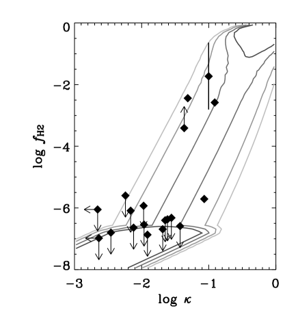
Figure 3: Likelihood contour on the $\log f_{\rm H_{2}}-\log\kappa$ diagram, when the density, temperature, and radiation field are varied in the range $1.5\leq\log n~{}[{\rm cm}^{-3}]\leq 2.5$, $1.5\leq\log T~{}[{\rm K}]\leq 3$, and $0.5\leq\log\chi\leq 1.5$, respectively. We adopt $N_{\rm H}=10^{21}$ cm^-2. The contours are drawn for four levels: 95%, 90%, 70%, and 50% of the sample is supposed to be in the regions corresponding to each level. The observational data points are the same as those in Figure 2.

4.3 Column density

Another important conclusion derived by Ledoux et al. (2003) is that the H i column density and the molecular fraction do not correlate. Therefore, we also present our model calculation for the $N_{\rm H}-f_{\rm H_{2}}$ relation. Since the difference in the dust-to-gas ratio reproduces a very different result, we only use the sample with $0.01<\kappa<0.1$. Here we assume $\kappa=0.03$. In Figure 4, we show our results with various gas density (the thick solid, dotted, and dashed lines represent the results with $n=100$, 30, and 300 cm^-3, respectively), where we assume that $T=100$ K, $\kappa=0.03$, and $\chi=10$. The thick lines underproduces the observed H₂ fraction of the H₂ detected objects, since the dust-to-gas ratio of those objects are systematically higher than that assumed. In particular, the data point with the bar ($z_{\rm abs}=1.973$ toward Q 0013$-$004) has the dust-to-gas ratio of $\kappa=0.099$. This data point can be reproduced by the thin dashed line produced with the same condition as the dashed line but with $\kappa=0.1$. As seen in Section 4.2, the same $n/\chi$ reproduces the same result with the other quantities fixed. Thus, we do not show the result for the various ISRF intensity $\chi$.

Figure 4: Relation between the molecular fraction and the H i column density. Only the observational sample with $0.01<\kappa<0.1$ is selected (squares). The upper and lower arrows represents the observational lower and upper limits for the molecular fraction, respectively. The thick solid, dotted, and dashed lines present our calculations with various gas density ($n=100$, 30, and 300, respectively). The gas temperature, dust-to-gas ratio and ISRF intensity are assumed to be $T=100$ K, $\kappa=0.03$, and $\chi=10$, respectively. The thin dashed line indicate the same calculation with the thick dashed line, but a higher dust-to-gas ratio of $\kappa=0.1$ is assumed. We also show the self-shielding condition by dotted line, above which the H₂ self-shielding effect becomes significant.

The thin dotted line in Figure 4 represents the relation $f_{\rm H_{2}}=f_{\rm H_{2}}^{\rm cr}$ (equation 6). Therefore, if a data point is above the thin dotted line, the H₂ is self-shielding the dissociating photons. We observe that the molecular fraction is very sensitive to the gas density and ISRF intensity, especially in the self-shielding regime. This sensitive dependence tends to erase the correlation between $f_{\rm H_{2}}$ and $N_{\rm H}$ in the observational sample and could explain the absence of correlation in the observational sample.

4.4 Possibility of warm phase

As mentioned in Section 3.3, our derived quantities are biased to the H₂ detected objects. As shown in Hirashita et al. (2003), H₂-rich regions are only confined in a small dense regions, whose gas temperature is $T\la 100$ K. However, Chengalur & Kanekar (2000) observationally derive the spin temperature $T\ga 1000$ K for a large part of their DLA sample and $T\sim 100$ K for a few DLAs, although the large beam size relative to the size of the QSO may tend to overestimate the spin temperature. Ledoux et al. (2002) find that the DLAs with H₂ detection are always dense ($n>30~{}{\rm cm}^{-3}$) and cool ($T<100$ K). Therefore, most of the DLAs may be warm except for the H₂ detected ones.

Based on a simulation suitable for DLAs, Hirashita et al. (2003) have shown that most ($\sim 90$%) of the regions are covered by warm and diffuse regions with $T\sim 1000$–10000 K and $n\sim 1$ cm^-3. In the warm phase, H₂ formation on dust is not efficient and H₂ formation occurs in gas phase (Liszt 2002; Cazaux & Tielens 2002). Therefore, we cannot put any constraint on the physical state of warm gas in the framework of this paper. The H₂ formation in gas phase occurs in the following route: ${\rm H}+{\rm e}^{-}\to{\rm H}^{-}+h\nu$, ${\rm H}^{-}+{\rm H}\to{\rm H}_{2}+{\rm H}^{+}$, and ${\rm H}^{+}+{\rm H}\to{\rm H}_{2}^{+}$, ${\rm H}_{2}^{+}+{\rm H}\to{\rm H}_{2}+{\rm H}^{+}$. Liszt (2002) shows that the gas phase reactions result in a molecular fraction $f_{\rm H_{2}}\sim 10^{-7}$–$10^{-8}$. This range is consistent with the data with upper limits of $f_{\rm H_{2}}$.

4.5 Lack of very H₂-rich DLAs?

The likelihood contours presented in Figure 3 suggests that some DLAs should be rich in H₂ ($\log f_{\rm H_{2}}\ga-1$) if the dust-to-gas ratio is around the Galactic value ($\log\kappa\ga-0.5$). However, all the objects in the sample have molecular fraction $\log f_{\rm H_{2}}<-1$. There are three possible explanations that we discuss in the following.

The first possibility of the lack of very molecule-rich DLAs is the contamination from the molecule-poor intercloud medium. If the contribution of intercloud medium to the column density is high, the molecular fraction is inferred to be low even if a molecule-rich region is present along the line of sight.

Secondly, a QSO selection effect might occur. If the dust-to-gas ratio is as high as $\log\kappa>-0.5$ and the column density is $N_{\rm H}=10^{21}~{}{\rm cm}^{-2}$, the optical depth of dust in UV is larger than 0.3 (equation 5). Therefore, QSO is effectively extinguished by dust if there is a dust-rich cloud in the line of sight. Such a population is also suggested by a numerical simulation (Cen et al. 2003). Observationally, it is a matter of debate whether the dust bias is large or not. Ellison et al. (2002) study optical colours of optically-selected QSO samples, and find that the effect of dust extinction of intervening absorbers is small. Fall et al. (1989) show a significant dust extinction of intervening DLAs by showing that QSOs with foreground DLAs tend to be redder than those without foreground DLAs.

The third possibility is concerned with the probability of detecting molecule-rich DLAs. Hirashita et al. (2003) have shown that the covering fraction of H₂-rich clouds in a galactic surface is $\la 10$%. Therefore, the probability that the line of sight passes through such clouds may be very low. Some very small molecule-rich clumps, which would be difficult to find as QSO absorption systems, are also found (e.g. Richter et al. 2003; Heithausen 2004). The probability distribution function of gas density and temperature should be treated by taking into account the covering fraction. The detailed treatment of such probability is left for the future work.

Extremely molecular-rich objects with $f_{\rm H_{2}}\sim 1$ might escape H i absorption detection (Schaye 2001). A new strategy will be required to detect such fully molecular clouds at high $z$. An observational strategy for high-$z$ molecular clouds with high column densities is discussed in Shibai et al. (2001).

4.6 Summary of our analysis

In order to summarise our analysis and for the observers’ convenience, we present Figure 5. Various physical states of gas could be discriminated on the $f_{\rm H_{2}}-\kappa$ (molecular fraction vs. dust-to-gas ratio) diagram. First of all, we should stress that this diagram is only useful to obtain the first result about the gas state of an absorption line system whose H₂ fraction and dust-to-gas ratio are constrained, or to obtain the statistical properties of gas phase of a sample of absorption systems. For the confirmation of gas state, more detailed analysis such as treatment of C i fine structure lines should be combined.

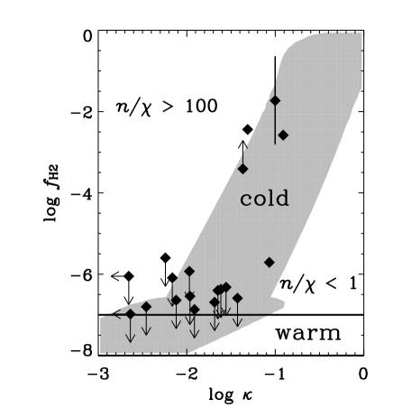
Figure 5: Summary of our analysis. If we obtain the molecular fraction and dust-to-gas ratio for an absorption system, we can roughly estimate the physical state of gas. This diagram should only be used to obtain the first rough estimate. The region marked with “cold” indicates the same area as the 90% level of Figure 3 (representative of a typical cold phase). The strip marked with “warm” indicates the typical range of $f_{\rm H_{2}}$ in a warm phase where H₂ is formed in gas phase (Liszt 2002). The other two regions are possibly characterised by the physical state, $n/\chi\ga 100$ and $n/\chi\la 1$ (see text for details).

In Figure 5, the shaded area shows the region where 90% of the gas with $1.5\leq\log n~{}[{\rm cm}^{-3}]\leq 2.5$, $1.5\leq\log T~{}[{\rm K}]\leq 3$, and $0.5\leq\log\chi\leq 1.5$ is predicted to be located (see Figure 3). Those ranges of the quantities are typical of H₂-detected objects and representative of “cold” gas. The strip indicated by “warm” shows the warm phase in which H₂ predominantly forms in the gas phase (we take the values from Liszt 2002). There is an overlapping region of the cold and warm states, and if a data point lies in this region, the warm and cold states are equally probable. There remain two regions not included neither in “cold” nor in “warm”. The upper region shows an enhancement of the molecular fraction, which requires a high H₂ formation rate and/or a low H₂ destruction rate. This condition is typically characterised with $n/\chi\ga 100$ if the gas temperature is favourable for the H₂ formation on dust grains ($\la 100$ K). On the other hand, the lower region marked with “$n/\chi<1$” indicates that the H₂ fraction is larger than the typical value in warm phase but lower than our likelihood range for cold gas. If a data point lies in this region, there could be the following three possibilities: (i) $n/\chi\la 1$ and $T\la 100$ K, so that the H₂ formation rate is suppressed because of a low density and/or the H₂ destruction rate is enhanced because of a high ISRF; (ii) $300\la T\la 500$ K, so that the H₂ formation on dust occurs only with a small rate; (iii) the cold and warm phases coexist in the line of sight. We can use this diagram as the “first quick look” for the physical state of gas if H₂ is detected in a system whose dust-to-gas ratio has been estimated.

5 STAR FORMATION

5.1 Star formation rate

The above results for the relation between molecular abundance and dust-to-gas ratio for DLAs strongly suggest that there are internal UV radiation sources originating from star formation activity (see also Ge & Bechtold 1997; Ledoux et al. 2002; Petitjean et al. 2002). Indeed, the cosmic UV background radiation intensity is typically $J_{21}\sim 1$ around $z\sim 3$. This corresponds to $\chi\simeq 3.1\times 10^{-2}$. The ISRF intensity is clearly larger than this, and the local heating sources such as stars dominates the ISRF. Assuming that the ISRF is produced by stars, we relate the ISRF with the SFR.

Hirashita, Buat, & Inoue (2003) have derived the relation between UV luminosity and SFR as

$${\rm SFR}=C_{2000}L_{2000}\,,$$ (19)

where $L_{2000}$ is the monochromatic luminosity at 2000 Å and $C_{2000}=2.03\times 10^{-40}$ [($M_{\odot}$ yr^-1)/(erg s^-1 Å^-1)] (under a Salpeter initial mass function with the stellar mass range of 0.1–100 $M_{\odot}$ and a constant star formation rate with the duration of $10^{8}$ yr; see also Iglesias-Páramo et al. 2004). The surface luminosity density, defined as the luminosity per surface area, can be roughly equated with the ISRF intensity (Appendix A). Therefore, the 2000 Å surface monochromatic luminosity density, $\Sigma_{\rm 2000}$, is estimated as

$$\Sigma_{2000}\simeq cu_{2000}=9.0\times 10^{-7}\chi~{}{\rm erg~{}cm}^{-2}~{}{\rm s}^{-1}~{}\mbox{\AA}^{-1}\,.$$ (20)

where we use the 2200 Å energy density in Habing (1968) for the normalisation of $u_{2000}$ (2000 Å monochromatic radiative energy density). Using equation (20), we obtain the surface density of SFR, $\Sigma_{\rm SFR}$:

$$\Sigma_{\rm SFR}=C_{2000}\Sigma_{2000}=1.7\times 10^{-3}\chi~{}M_{\odot}~{}{\rm yr}^{-1}~{}{\rm kpc}^{-2}\,.$$ (21)

Indeed, this roughly gives the Galactic surface SFR density ($\sim 10^{-3}~{}M_{\odot}~{}{\rm yr}^{-1}~{}{\rm kpc}^{-2}$; Burkert, Truran, & Hensler 1992) if we assume a typical ISRF intensity of the solar vicinity ($\chi=1$). But some observational data indicate higher Galactic surface SFR in the solar vicinity such as $\sim 5\times 10^{-3}~{}M_{\odot}~{}{\rm yr}^{-1}~{}{\rm kpc}^{-2}$ (Smith et al. 1978). The general ISRF in the Galaxy could be systematically higher (i.e. $\chi>1$; Shibai et al. 1999).

Wolfe et al. (2003) have derived the calibration $\Sigma_{\rm SFR}=2.5\times 10^{-3}\chi~{}M_{\odot}~{}{\rm yr}^{-1}~{}{\rm kpc}^{-2}$. The difference comes from the different assumption on the IMF and the different stellar mass-luminosity relation. However the difference in only 0.17 in the logarithmic scale.

The probable range of the radiation field constrained in section 4.2 is $0.5\la\log\chi\la 1.5$. This range predicts the surface SFR density, $5\times 10^{-3}~{}M_{\odot}~{}{\rm yr}^{-1}~{}{\rm kpc}^{-2}\la\Sigma_{\rm SFR}\la 5\times 10^{-2}~{}M_{\odot}~{}{\rm yr}^{-1}~{}{\rm kpc}^{-2}$. Wolfe et al. (2003a) derive the UV radiation field from C ii* absorption line. Their analysis is dependent on the assumed phase (cool or warm) of the ISM. The calculated SFR differs by an order of magnitude between the cool and warm media. Based on their results, Wolfe et al. (2003b) have suggested that the probable range of the SFRs of their sample is $10^{-3}\la\Sigma_{\rm SFR}~{}[M_{\odot}~{}{\rm yr}^{-1}~{}{\rm kpc}^{-2}]\la 10^{-2}$. This range is roughly consistent with our range considering the uncertainty in the assumed physical state of gas. A numerical work by Nagamine, Springel, & Hernquist (2004) explains the SFR theoretically. Our estimate provides an independent observational calculation for the SFR of DLAs.

Assuming a typical radius of $R=3$ kpc for DLAs (Kulkarni et al. 2000), we obtain the SFR $\Sigma_{\rm SFR}\pi R^{2}\sim 0.1$–1 $M_{\odot}~{}{\rm yr}^{-1}$. This range is broadly consistent with the upper limits obtained by some imaging observations of DLAs (Bunker et al. 1999; Kulkarni et al. 2000; Bouché et al. 2001).

5.2 Comparison with other SFR estimates

Wolfe et al. (2003a) have estimated the SFR of a sample of DLAs by using C ii* absorption intensity. They consider the balance between the cooling rate dominated by [C ii] fine structure line emission and the heating rate dominated by photoelectric heating of a UV radiation field. Since our method for SFR estimate is independent of theirs, the consistency between the two methods is interesting to explore. Wolfe et al. (2003a) investigate two thermally stable states, WNM (warm neutral medium) and CNM (cold neutral medium), adopting the scheme of Wolfire et al. (1995). There are three overlapping samples between Wolfe et al. (2003a) and Ledoux et al. (2003) as shown below.

5.2.1 Q 0347$-$383 ($z_{\rm abs}=3.025$)

Some H₂ lines are detected in this object, and we have derived $\chi=15$ (Section 3.2), which is equivalent to $\log\Sigma_{\rm SFR}~{}[M_{\odot}~{}{\rm yr}^{-1}~{}{\rm kpc}^{-2}]=-1.6$. Wolfe et al. (2003a) derive $\log\Sigma_{\rm SFR}~{}[M_{\odot}~{}{\rm yr}^{-1}~{}{\rm kpc}^{-2}]=-1.3$ and $-2.2$ for the WNM and CNM, respectively. Our estimated temperature $T=400$–800 K is higher than the typical value for CNM ($\sim 100$ K) and lower than the WNM. In any case, our estimate is between the two values of Wolfe et al. (2003a).3

5.2.2 Q 1223+178 ($z_{\rm abs}=2.466$)

For this object, the depletion factor is extremely small (${\rm[Fe/Zn]}=-0.07\pm 0.21$), and the metallicity is also small (${\rm[Zn/H]}=-1.63\pm 0.11$) (Ledoux et al. 2003). Thus, it is expected that dust-to-gas ratio of this object is extremely small. Moreover, if we assume the above metal abundances, we obtain $\log\kappa=-2.46$. With this dust abundance, the formation of H₂ through H^- could be an important process. The SFR cannot be estimated by our method.

5.2.3 Q 1232$+$082 ($z_{\rm abs}=2.338$)

In Section 3.2, we have estimated the radiation field to be $\chi\leq 64$, which is equivalent to the surface SFR density $\log\Sigma_{\rm SFR}~{}[M_{\odot}~{}{\rm yr}^{-1}~{}{\rm kpc}^{-2}]\leq-0.96$. The low excitation temperature ($T_{10}=185$ K) indicates that the gas in the CNM. The CNM solution of Wolfe et al. (2003a) shows $\log\Sigma_{\rm SFR}~{}[M_{\odot}~{}{\rm yr}^{-1}~{}{\rm kpc}^{-2}]=-1.9$, consistent with our upper limit.

5.3 Cosmological implications

Wolfe et al. (2003b) have extended their discussion on the SFR in DLAs to a cosmological context. They have found that the hypothesis that most of the DLAs are in WNM is ruled out because it would conflict with background light constraint. On the other hand, Chengalur & Kanekar (2000) have observationally shown that a large part of their DLAs have a temperature similar to WNM. Hirashita et al. (2003), by using detailed numerical simulations, have also argued that the probability to observe the CNM of a DLA is small because the tiny covering fraction of such phase. Their calculation also shows that H₂ detected objects are biased to the CNM, and is consistent with the estimates in Section 3.2. Most of the H₂ deficient DLAs may be in the WNM. Thus at the moment, there seems to be tension between the CNM and WNM hypotheses, which requires additional work in order to be relaxed. A composite analysis of fine-structure excitation and H₂ may be required to confirm our results of a simple statistical approach.

In spite of such an uncertainty, it is interesting to note that the star formation activity in DLAs can be investigated via our treatment of H₂ formation and destruction rates. The surface SFR density derived by us is comparable to that inferred in Wolfe et al. (2003a), who have suggested that DLAs are an important population in the cosmic star formation (and metal production) history (see also Pei & Fall 1995; Pei, Fall, & Hauser 1999). The SFR is much lower than forming elliptical galaxies as calculated by Arimoto & Yoshii (1987), but more similar to spiral galaxies. In the context of the hierarchical structure formation, Nagamine et al. (2004) have explained the SFR of DLAs by a cosmological simulation, and they also show that the SFR of a DLA is generally smaller than that of a typical Lyman break galaxies ($\sim 50~{}M_{\odot}~{}{\rm yr}^{-1}$) (but see Schaye 2004). According to their simulation, the host halo mass of DLAs spans over a wide range from $\sim 10^{9}~{}M_{\odot}$ to $\sim 10^{12}~{}M_{\odot}$. Another theoretical calculation by Hirashita & Ferrara (2002) show that high-$z$ dwarf galaxies whose total mass of dark halo is around $10^{9}~{}M_{\odot}$ has a SFR similar to that estimated in Section 5.1.

Our statistical work in this paper will be extended to the cosmological star formation history and some observational consequences (see also Ferrara et al. 1999). The redshift evolution of H₂ abundance and the relation between metals and H₂ (Curran et al. 2004) can also be used to constrain the cosmological SFR.

6 SUMMARY

We have modeled the H₂ abundance of QSO absorption line systems and compared our model calculations with observational samples of damped Ly$\alpha$ systems (DLAs) and sub-DLAs. We have derived the H₂ abundance, $f_{\rm H_{2}}$, as a function of dust-to-gas ratio, $\kappa$ (normalized to the Galactic value) considering H₂ self-shielding and dust extinction against dissociating photons. The $f_{\rm H_{2}}-\kappa$ relation depends on the gas density ($n$) and temperature ($T$), and the ISRF intensity ($\chi$: normalised to the Galactic value). Our aim has been to constrain those quantities by using H₂ data. Treating the data of H₂ excitation states of the H₂ detected objects, we adopt $1.5\la\log n~{}[{\rm cm}^{-3}]\la 2.5$, $1.5\la\log T~{}[{\rm K}]\la 3$, and $0.5\la\log\chi\la 1.5$. From the comparison with data, we have found that the observational $f_{\rm H_{2}}$ – $\kappa$ relation is naturally explained by the above range. The efficient photodissociation by the ISRF can explain the extremely small H₂ abundance ($f_{\rm H_{2}}\la 10^{-6}$) observed for $\kappa\la 1/30$. We have also succeeded in explaining the rapid increase of H₂ abundance for $\kappa\ga 1/30$ by the effect of self-shielding of H₂ dissociating photons. Because of a nonlinear dependence of self-shielding on the physical quantities, a large scatter of H₂ fraction is reproduced. However, we should note that the above parameter range may be biased to the cold gas favourable for H₂ formation. It is still possible that most of the H₂ deficient DLAs and sub-DLAs might be in a diffuse and warm state.

We finally propose to estimate star formation rates (SFRs) of (sub-)DLAs from H₂ observations. The SFRs estimated by our method are compared with those derived by Wolfe et al. (2003a). Two common samples give roughly consistent SFRs. The strength of UV field indicates a surface SFR density: $5\times 10^{-3}$–$5\times 10^{-2}~{}M_{\odot}~{}{\rm yr}^{-1}~{}{\rm kpc}^{-2}$. Therefore, DLAs are actually star-forming objects. The SFR is smaller than typical Lyman break galaxies, but DLAs may be a major population responsible for star formation in the high-$z$ universe.

Appendix A SURFACE LUMINOSITY DENSITY AND RADIATION FIELD

In the text, we have equated the surface luminosity density $\Sigma$ with the interstellar radiation field (ISRF) intensity $cu$. However, it is not obvious a priori that this assumption is correct. If the radiation from a stars is isotropic and the dust extinction is neglected, the ISRF intensity at the position $\bm{r}$, $cu(\bm{r})$, is expressed as

$$cu(\bm{r})=\int d^{3}\bm{r}^{\prime}\frac{\rho(\bm{r}^{\prime})}{4\pi|\bm{r}^{\prime}-\bm{r}|^{2}}\,,$$ (22)

where $\rho(\bm{r})$ is the spatial luminosity density of stars ($\rho(\bm{r})d^{3}\bm{r}$ is the luminosity in the volume element $d^{3}\bm{r}$).

One of the largest uncertainties is the spatial distribution of radiating sources. Therefore, in the following discussions, we derive the relation between $\Sigma$ and $cu$ under two representative geometries of source distribution: spherical and disc-like distributions.

A.1 Spherical distribution

In the spherical symmetric distribution, we can calculate the ISRF intensity at the centre of the sphere by

$$cu=\int_{0}^{R_{0}}dR\,4\pi R^{2}\frac{\rho(R)}{4\pi R^{2}}=\int_{0}^{R_{0}}dR\,\rho(R)\,,$$ (23)

where $R_{0}$ is the radius of the whole emitting region. The right-hand side gives a rough estimate of the surface luminosity density (denoted as $\Sigma$), and therefore, the ISRF can be equated with the surface luminosity density (i.e. $\Sigma\simeq cu$).

A.2 Disc-like distribution

In the disc-like distribution, we can calculate the ISRF intensity at the centre of the disc by

$$cu=\int_{0}^{R_{0}}dR\,2\pi R\int_{-h}^{h}dz\frac{\rho(R,\,z)}{4\pi(R^{2}+z^{2})}\,,$$ (24)

where $2h$ is the disc thickness, and $R_{0}$ is the disc radius. If we assume for simplicity that $\rho$ is constant, we obtain analytically

$$cu=\rho h\left\{\frac{R_{0}}{h}\arctan\frac{h}{R_{0}}+\frac{1}{2}\ln\left[\left(\frac{R_{0}}{h}\right)^{2}+1\right]\right\}\,.$$ (25)

The galactic discs usually satisfy $R_{0}\gg h$, so that the above equation is approximated as

$$cu\simeq\rho h\left(1+\ln\frac{R_{0}}{h}\right)\,.$$ (26)

The dependence on $R_{0}/h$ is very weak, and even if we assume a very thin disc such as $R_{0}/h=100$, we obtain $cu\simeq 5.6\rho h$. The surface luminosity density can be typically estimated by $\Sigma\simeq 2\rho h$. Therefore, $cu$ and $\Sigma$ have the same order of magnitude (different by a factor of $\la 3$).

The above discussions justify our simple assumption $cu=\Sigma$ in the text.

Appendix B LIKELIHOOD FORMULATION

We consider a set of $n$ physical quantities, $\bm{x}=(x_{1},\,\cdots,\,x_{n})$. Suppose that those quantities are determined by a set of $m$ parameters, $\bm{y}=(y_{1},\,\cdots,\,y_{m})$, each of which has a reasonable range $y_{i}^{\rm min}\leq y_{i}\leq y_{i}^{\rm max}$ ($i=1,\,\cdots,\,m$). The two sets of quantities are related to the following function $f$:

$$\bm{y}=f(\bm{x})\,.$$ (27)

We divide $\bm{x}$ and $\bm{y}$ into $N+1$ and $M+1$ bins, respectively:

$$x_{i}^{j} \equiv x_{i}^{\rm min}+\frac{j}{N}(x_{i}^{\rm max}-x_{i}^{\rm min})~{}~{}~{}(j=0,\,\cdots,\,N)\,.$$ (28)

$$y_{i}^{k} \equiv y_{i}^{\rm min}+\frac{k}{M}(y_{i}^{\rm max}-y_{i}^{\rm min})~{}~{}~{}(k=0,\,\cdots,\,M)\,.$$ (29)

The $j$-th and $k$-th bins of $x_{i}$ and $y_{i}$ can be defined as the range $[x_{i}^{j-1},\,x_{i}^{j}]$ ($j=1,\,\cdots,\,N$) and $[y_{i}^{k-1},\,y_{i}^{k}]$ ($k=1,\,\cdots,\,M$), respectively. Any $N$-dimensional bin of $\bm{x}$ can be specified by a set of $N$ integers $(j_{1},\,\cdots,\,j_{n})$. We represent the value of $\bm{y}$ in each bin with the median as

$$\bm{y}(k_{1},\,\cdots,\,k_{m})\equiv\left(\frac{y_{1}^{k_{1}-1}+y_{1}^{k_{1}}}{2},\,\cdots,\,\frac{y_{m}^{k_{m}-1}+y_{m}^{k_{m}}}{2}\right)\,.$$ (30)

We define $N(j_{1},\,\cdots,\,j_{n})$ as the number of the combination of $m$ integers $(k_{1},\,\cdots,\,k_{m})$ such that $f(\bm{y}(k_{1},\,\cdots,\,k_{m}))$ is in the $n$-dimensional bin $(j_{1},\,\cdots,\,j_{n})$ of $\bm{x}$. Then the likelihood of $\bm{x}(j_{1},\,\cdots,\,j_{n})$, $P(j_{1},\,\cdots,\,j_{n})$, can be defined as

$$P(j_{1},\,\cdots,\,j_{n})\equiv\frac{N(j_{1},\,\cdots,\,j_{n})}{\sum_{j_{1},\,\cdots,\,j_{n}}N(j_{1},\,\cdots,\,j_{n})}\,.$$ (31)

Let $\partial S(p)$ be a contour surface of $P=p$ ($(n-1)$-dimensional surface), and let $S(p)$ be the area where surrounded by $\partial S(p)$. Then, the following sum Prob($S$) gives the probability that the data $\bm{x}$ lies in $S$:

$${\rm Prob}(S)\equiv\sum_{\bm{x}\in S}P(\bm{x}(j_{1},\,\cdots,\,j_{n}))\,.$$ (32)

References

- [Abel et al.(2004)] Abel, N. P., Brogan, C. L., Ferland, G. J., O’Dell, C. R., Shaw, G., & Troland, T. H. 2004, ApJ, 609, 247
- [Abel et al.(1997)] Abel, T., Anninos, P., Zhang, Y., Norman, M. L. 1997, NewA, 2, 181
- [André et al.(2004)] André, M. K. et al. 2004, A&A, 422, 483
- [Arimoto & Yoshii(1987)] Arimoto, N., & Yoshii, Y. 1987, A&A, 173, 23
- [Bianchi et al.(2001)] Bianchi, S., Cristiani, S., & Kim, T.-S. 2001, A&A, 376, 1
- [Black et al.(1987)] Black, J. H., Chaffee, F. H. Jr., & Foltz, C. B. 1987, ApJ, 317, 442
- [Bouché(2001)] Bouché, N., Lowenthal, J. D., Bershady, M. A., Churchill, C. W., & Steidel, C. C. 2001, ApJ, 550, 585
- [Browning et al.(2003)] Browning, M. K., Tumlinson, J., & Shull, J. M. 2003, ApJ, 582, 810
- [Bunker et al.(1999)] Bunker, A. J., Warren, S. J., Clements, D. L., Williger, G. M., & Hewett, P. C. 1999, MNRAS, 309, 875
- [Burbidge et al.(1996)] Burbidge, E. M., Beaver, E. A., Cohen, R. D., Junkkarinen, V. T., & Lyons, R. W. 1996, AJ, 112, 2533
- [Cazaux & Tielens(2002)] Cazaux, S., & Tielens, A. G. G. M. 2002, ApJ, 575, L29
- [Cen et al.(2003)] Cen, R., Ostriker, J. P., Prochaska, J. X., & Wolfe, A. M. 2003, ApJ, 598, 741
- [Chengalur & Kanekar(2000)] Chengalur, J. N., & Kanekar, N. 2000 MNRAS, 318, 303
- [Cooke et al.(1997)] Cooke, A. J., Espey, B., & Carswell, R. F. 1997, MNRAS, 284, 552
- [Curran et al.(2004)] Curran, S. J., Webb, J. K., Murphy, M. T., & Carswell, R. F. 2004, MNRAS, 351, L24
- [Draine & Bertoldi(1996)] Draine, B. T., & Bertoldi, F. 1996, ApJ, 468, 269
- [Draine & Lee(1984)] Draine, B. T., & Lee, H. M. 1984, ApJ, 285, 89
- [Draptz et al.(1977)] Drapatz, S., & Michel, K. W. 1977, A&A, 56, 353
- [Ellison et al.(2002)] Ellison, S. L., Yan, L., Hook, I. M., Pettini, M., Wall, J. V., & Shaver, P. 2002, A&A, 383, 91
- [Fall et al.(1989)] Fall, S. M, Pei, Y. C. & McMahon, R. G. 1989, ApJ, 341, L5
- [Ferrara et al.(1999)] Ferrara, A., Nath, B., Sethi, S. K., & Shchekinov, Y. 1999, MNRAS, 303, 301
- [Gardner et al.(2001)] Gardner, J. P., Katz, N., Hernquist, L., & Weinberg, D. H. 2001, ApJ, 559, 131
- [Ge & Bechtold(1997)] Ge, J., & Bechtold, J. 1997, ApJ, 477, L73
- [Ge et al.(2001)] Ge, J., Bechtold, J., & Kulkarni, P. 2001, ApJ, 547, L1
- [Giallongo et al.(1996)] Giallongo, E., Cristiani, S., D’Odorico, S., Fontana, A., & Savaglio, S. 1996, ApJ, 466, 46
- [Gry et al.(2002)] Gry, C., Boulanger, F., Nehmé, C., Pineau de Forêts, G., Habart, E., & Falgarone, E. 2002, A&A, 391, 675
- [Haardt & Madau(1996)] Haardt, F. & Madau, P. 1996, ApJ, 461, 20
- [Habing(1968)] Habing, H. J. 1968, Bull. Astr. Inst. Netherlands, 19, 421
- [Haehnelt et al.(1998)] Haehnelt, M. G., Steinmetz, M., & Rauch, M. 1998, ApJ, 495, 647
- [Heithausen(2004)] Heithausen, A. 2004, ApJ, 606, L13
- [Hirashita et al.(2003)] Hirashita, H., Buat, V., & Inoue, A. K. 2003, A&A, 410, 83
- [Hirashita & Ferrara(2002)] Hirashita, H., & Ferrara, A. 2002, MNRAS, 337, 921
- [Hirashita et al.(2003)] Hirashita, H., Ferrara, A., Wada, K., & Richter, P. 2003, MNRAS, 341, L18
- [Hirashita & Hunt(2004)] Hirashita, H., & Hunt, L. K. 2004, A&A, 421, 555
- [Hollenbach & McKee(1979)] Hollenbach, D. J., & McKee, C. F. 1979, ApJS, 41, 555
- [Iglesias-Páramo et al.(2004)] Iglesias-Páramo, J., Buat, V., Donas, J., Boselli, A., & Milliard, B. 2004, A&A, 419, 109
- [Jura(1974)] Jura, M. 1974, ApJ, 191, 375
- [Jura(1975)] Jura, M. 1975, ApJ, 197, 581
- [Kulkarni et al.(2000)] Kulkarni, V. P., Hill, J. M., Schneider, G., Weymann, R. J., Storrie-Lombardi, L. J., Rieke, M. J., Thompson, R. I., & Jannuzi, B. T. 2000, ApJ, 536, 36
- [Lanzetta et al.(1989)] Lanzetta, K. M., Wolfe, A. M., & Turnshek, D. A. 1989, ApJ, 344, 277
- [Lanzetta et al.(1995)] Lanzetta, K. M., Wolfe, A. M., & Turnshek, D. A. 1995, ApJ, 440, 435
- [Ledoux et al.(2002)] Ledoux, C., Srianand, R., & Petitjean, P. 2002, A&A, 392, 781
- [Ledoux et al.(2003)] Ledoux, C., Petitjean, P., & Srianand, R. 2003, MNRAS, 346, 209
- [Levshakov et al.(2002)] Levshakov, S. A., Dessauges-Zavadsky, M., D’Odorico, S., & Molaro, P. 2002, ApJ, 565, 696
- [Levshakov et al.(2000)] Levshakov, S. A., Molaro, P., Centurión, M., D’Odorico, S., Bonifacio, P., & Vladilo, G. 2000, A&A, 361, 803
- [Liszt(2002)] Liszt, H. 2002, A&A, 389, 393
- [Lu et al.(1996)] Lu, L., Sargent, W. L. W., Barlow, T. A., Churchill, C. W., & Vogt, S. S. 1996, ApJS, 107, 475
- [Marggraf et al.(2004)] Marggraf, O., Bluhm, H., & de Boer, K. S. 2004, A&A, 416, 251
- [McKee & Ostriker(1977)] McKee, C. F., & Ostriker, J. P. 1977, ApJ, 218, 148
- [Møller et al.(2002)] Møller, P., Warren, S. J., Fall, S. M., Fynbo, J. U., & Jakobsen, P. 2002, ApJ, 574, 51
- [Murphy & Liske(2004)] Murphy, M. T., & Liske, J. 2004, MNRAS, submitted
- [Nagamine et al.(2004)] Nagamine, K., Springel, V., & Hernquist, L. 2004, MNRAS, 348, 435
- [Okoshi et al.(2004)] Okoshi, K., Nagashima, M., Gouda, N., & Yoshioka, S. 2004, ApJ, 603, 12
- [Omukai(2000)] Omukai, K. 2000, ApJ, 534, 809
- [Pei & Fall(1995)] Pei, Y. C., & Fall, S. M. 1995, ApJ, 454, 69
- [Pei, Fall, & Hauser(1999)] Pei, Y. C., Fall, S. M., & Hauser, M. G. 1999, ApJ, 522, 604
- [Péroux et al.(2003)] Péroux, C., McMahon, R. G., Storrie-Lombardi, L. J., & Irwin, M. J. 2003, MNRAS, 346, 1103
- [Petitjean et al.(2000)] Petitjean, P., Srianand, R., & Ledoux, C. 2000, A&A, 364, L26
- [Petitjean et al.(2002)] Petitjean, P., Srianand, R., & Ledoux, C. 2002, MNRAS, 332, 383
- [Pettini et al.(1999)] Pettini, M., Ellison, S. L., Steidel, C. C., & Bowen, D. V. 1999, ApJ, 510, 576
- [Pettini et al.(1994)] Pettini, M. H., Smith, L. J., Hunstead, R. W., & King, D. L. 1994, ApJ, 426, 79
- [Prochaska & Wolfe(2002)] Prochaska, J. X., & Wolfe, A. M. 2002, ApJ, 566, 68
- [Quast et al.(2002)] Quast, R., Baade, R., & Reimers, D. 2002, A&A, 386, 796
- [Rao et al.(2003)] Rao, S. M., Nestor, D. B., Turnshek, D. A., Lane, W. M., Monier, E. M., & Bergeron, J. 2003, ApJ, 595, 94
- [Reimers et al.(2003)] Reimers, D., Baade, R., Quast, R., & Levshakov, S. A. 2003, A&A, 410, 785
- [Richter 2000] Richter, P., 2000, A&A, 359, 1111
- [Richter et al.(2003a)] Richter, P., Sembach, K. R., & Howk, J. C. 2003, A&A, 405, 1013
- [Richter et al.(2003b)] Richter, P., Wakker, B. P., Savage, B. D., Sembach, K. R., 2003, ApJ, 586, 230
- [Salucci & Persic(1999)] Salucci, P., & Persic, M. 1999, MNRAS, 309, 923
- [Schaye(2001)] Schaye, J. 2001, ApJ, 562, L95
- [Schaye(2004)] Schaye, J. 2004, ApJ, submitted
- [Scott et al.(2000)] Scott, J., Bechtold, J., Dobrzycki, A., & Kulkarni, V. P. 2000, ApJS, 130, 67
- [Scott et al.(2002)] Scott, J., Bechtold, J., Morita, M., Dobrzycki, A., & Kulkarni, V. P. 2002, ApJ, 571, 665
- [Shibai et al.(1999)] Shibai, H., Okumura, K., & Onaka, T. 1999, in T. Nakamoto, ed., Star Formation 1999, Nobeyama, Nobeyama Radio Observatory, p. 67
- [Shibai et al.(2001)] Shibai, H., Takeuchi, T. T., Rengarajan, T. N., & Hirashita, H. 2001, PASJ, 53, 589
- [Smith et al.(1978)] Smith, L. F., Biermann, P., & Mezger, P. G. 1978, A&A, 66, 65
- [Spitzer(1978)] Spitzer, L., Jr. 1978, Physical Processes in the Interstallar Medium, Wiley, New York
- [Spitzer & Zweibel(1974)] Spitzer, L., Jr., & Zweibel, E. G. 1974, ApJ, 191, L127
- [Srianand et al.(2000)] Srianand, R., Petitjean, P., & Ledoux, C. 2000, Nat, 408, 931
- [Storrie-Lombardi & Wolfe(2002)] Storrie-Lombardi, L. J., & Wolfe, A. 2000, ApJ, 543, 552
- [Takeuchi et al.(2003)] Takeuchi, T. T., Hirashita, H., Ishii, T. T., Hunt, L. K., & Ferrara, A. 2003, MNRAS, 343, 839
- [Tumlinson et al. 2002] Tumlinson, J., et al., 2002, ApJ, 566, 857
- [Varshalovich et al.(2001)] Varshalovich, D. A., Ivanchik, A. V., Petitjean, P., Srianand, R., & Ledoux, C. 2001, Astron. Lett., 27, 683
- [Vladilo(2002)] Vladilo, G. 2002, A&A, 391, 407
- [Wada & Norman(2001)] Wada, K., & Norman, C. A. 2001, ApJ, 546, 172
- [Wolfe et al.(2003a)] Wolfe, A. M., Prochaska, J. X., & Gawiser, E. 2003a, ApJ, 593, 215
- [Wolfe et al.(2003b)] Wolfe, A. M., Gawiser, E., & Prochaska, J. X. 2003b, ApJ, 593, 235
- [Wolfe et al.(1986)] Wolfe, A. M., Turnshek, D. A., Smith, H. E., & Cohen, R. D. 1986, ApJ, 61, 249
- [Wolfire et al.(1995)] Wolfire, M. G., Hollenbach, D., McKee, C. F., Tielens, A. G. G. M., & Bakes, E. L. O. 1995, ApJ, 443, 152
- [Zuo et al.(1997)] Zuo, L., Beaver, E. A., Burbidge, E. M., Cohen, R. D., Junkkarinen, V. T., & Lyons, R. W. 1997, ApJ, 477, 568