Toward Understanding Environmental Effects in SDSS Clusters

We find clusters and superclusters of galaxies using the Data Release 1 of the Sloan Digital Sky Survey. We calculate a low-resolution density field with a smoothing length of 10 $h^{-1}$ Mpc to characterise the density of the cluster environment. We determine the luminosity function of clusters, and investigate properties of clusters in various environments. We find that clusters in a high-density environment have a luminosity a factor of $\sim 5$ higher than in a low-density environment. We also study clusters and superclusters in numerical simulations. Simulated clusters in a high-density environment are also more massive than those in a low-density environment. Comparison of the density distribution at various epochs in simulations shows that in large low-density regions (voids) dynamical evolution is very slow and stops at an early epoch. In contrast, in large regions of higher density (superclusters) dynamical evolution starts early and continues until the present; here particles cluster early, and by merging of smaller groups very rich systems of galaxies form.

1 Introduction

Clusters and superclusters of galaxies are the basic building blocks of the Universe on cosmological scales. The first catalogues of clusters of galaxies by Abell (abell (1958), aco (1989)) and Zwicky et al. (1961– (68)) were constructed by visual inspection of the Palomar Observatory Sky Survey plates. Modern surveys of galaxies, such as the Las Campanas Redshift Survey (LCRS), the Sloan Digital Sky Survey (SDSS) and the two-degree-field (2dF) Galaxy Redshift Survey, enable us to define groups, clusters and superclusters of galaxies and to investigate properties of these galaxy systems in various large-scale environments.

Studies of the dependence of properties of galaxy systems on the density of the large-scale environment have been made by Einasto et al. 2003a , 2003b , 2003c , 2003d (hereafter E03a, E03b, E03c and E03d, respectively), using the Early Data Release (Stoughton et al. s02 (2002))of the SDSS and the Las Campanas Redshift Survey. These studies demonstrated the presence of environmental effects in clusters – clusters in a high-density environment are richer and larger than in a low-density environment.

The present study has three goals. First of all, we shall check the results obtained by E03a and E03b using a more accurate definition of groups and clusters. E03a and E03b found clusters of galaxies as density enhancements in the high-resolution 2-dimensional density field. Such a definition has its restrictions, as in some cases clusters may overlap in the projection direction, and cluster properties may be distorted. In contrast to previous studies we shall now define groups and clusters in the conventional way using the full 3-dimensional data on the distribution of galaxies. In this analysis we shall use galaxy samples of the Data Release 1 of the Sloan Digital Sky Survey (DR1 of SDSS, Abazajian et al. abazajian03 (2003)), and shall investigate properties of these systems in relation to the large-scale environment, from rich superclusters to poor filaments of loose groups in voids.

The second goal of our study is to compare properties of clusters and superclusters with properties of similar systems found in N-body simulations of structure evolution. In particular, we are interested in the relationship of cluster properties and their large-scale environment. We define DM-haloes in simulations in the same way as groups and clusters were defined in real galaxy samples, and superclusters as large over-density regions of the smoothed density field. This comparison of real and simulated cluster properties complements a similar study by Einasto et al. (2004b ) where a different method was used to characterise the density of the environment.

The third and ultimate goal of the present study is to try to find an explanation for the environmental dependence of cluster luminosities. For this purpose we shall compare the evolution of groups and clusters in high- and low-density regions. Also we shall compare the distribution of particles located in systems of various richness in high- and low-density environments. This comparison shall be done for various epochs, which gives us the possibility to follow the evolution in regions of various global density.

In the next Section we describe the SDSS DR1 sample of galaxies and the method used to find groups/clusters of galaxies. Here we describe also the N-body simulations of the structure evolution used to compare observations with models. In Section 3 we describe the density field of the SDSS DR1, and properties of clusters of the SDSS DR1. In Section 4 we compare the properties of observed clusters with those of similar objects found in simulations. In Section 5 we follow the evolution of high- and low-density regions in an attempt to understand the mechanism behind the environmental effects in cluster and galaxy luminosities. We discuss our results and compare them with previous studies in Section 6. The last Section brings our conclusions. High-resolution colored figures of the SDSS DR1 density fields are available at the web-site of Tartu Observatory (http://www.aai.ee/$\sim$einasto). Preliminary results of this study were reported at the conference on the Zone of Avoidance by Einasto et al. (2004a ).

2 Data

2.1 SDSS DR1 data

The SDSS Data Release 1 consists of two slices of about 2.5 degrees thick and 65–105 degrees wide, centered on the celestial equator, and of several regions at higher declinations. In the present study we have used only the equatorial slices. We extracted the Northern and Southern slice samples from the full DR1 sample, using the following criteria: the redshift interval $1000\leq cz\leq 60000$ km s^-1, the Petrosian $r^{*}$-magnitude interval $13.0\leq r^{*}\leq 17.7$, the right ascension and declination intervals $145^{\circ}\leq RA\leq 250.0^{\circ}$ and $-1.25^{\circ}\leq DEC\leq 1.25^{\circ}$ for the Northern slice, and $350^{\circ}\leq RA\leq 55.0^{\circ}$ and $-1.25^{\circ}\leq DEC\leq 1.25^{\circ}$ for the Southern slice. The number of galaxies extracted ($N_{\rm gal}$) and the length of the slice in the right ascension ($\Delta RA$) are given in Table 1.

Table 1: Data on the SDSS DR1 galaxies, clusters and superclusters

Sample $$\Delta$$RA

SDSS.N 19783 2754 10232 26

SDSS.S 11562 1451 6202 16

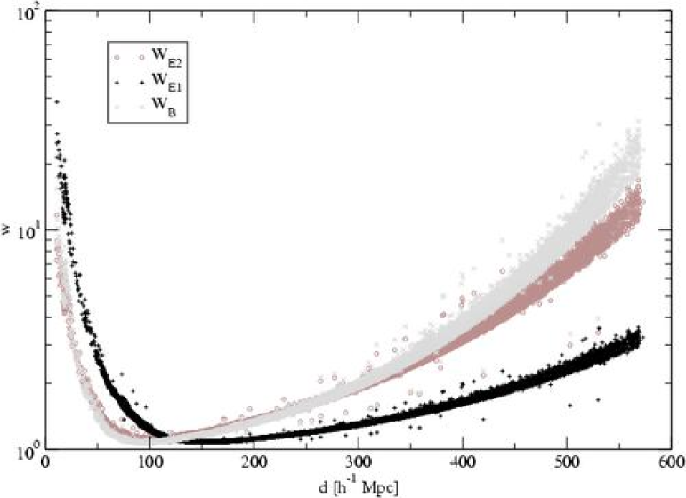
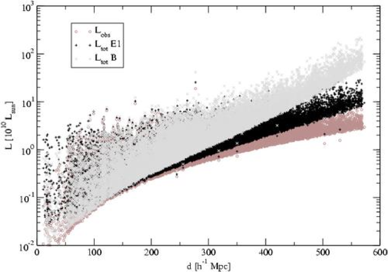
Figure 1: The left panel shows the weights of galaxies used to correct for invisible galaxies outside the observational window. Black symbols show the weights for the Einasto set E1 of the Schechter parameters (used to find total luminosities of clusters); light gray and dark gray symbols show the weights for the Blanton B and the Einasto set E2 of the Schechter function parameters, respectively (the weights calculated with the set E2 were used to find the low-resolution density field). In the right panel we plot luminosities of galaxies: dark gray symbols show the observed luminosities, light gray and black symbols show the expected total luminosities, obtained using the Blanton B and the Einasto E1 sets of the Schechter function parameters.

Table 2: Data on N-body DM-haloes and superclusters

Sample $$L\leavevmode\nobreak\ [Mpc/h]$$

M100 100 0.30 0.70 0.80 0.70 3.98 8 2459

M200A 200 0.30 0.70 0.80 0.70 3.98

M200B 200 0.27 0.73 0.84 0.71 3.59 20 12306

The SDSS data reduction procedure consists of several steps: (1) calculation of the distance, the absolute magnitude, and the weight factor for each galaxy of the sample; (2) finding groups/clusters of galaxies using the friends-of-friends algorithm; (3) calculation of the density field using an appropriate kernel and a chosen smoothing length. When calculating luminosities of galaxies we regard every galaxy as a visible member of a density enhancement (group or cluster) within the visible range of absolute magnitudes, $M_{1}$ and $M_{2}$, corresponding to the observational window of apparent magnitudes at the distance of the galaxy. This assumption is based on observations of nearby galaxies, which indicate that practically all field galaxies belong to poor groups like our own Galaxy, where one bright galaxy is surrounded by a number of faint satellites. Using this assumption, we find groups and clusters with their haloes, as single giant galaxies with their companions, or groups/clusters with their faint members. Further, we assume that the luminosity function derived for a representative volume can be applied also for individual groups and galaxies.

The calculation of the distances, absolute magnitudes and weight factors of galaxies was described in detail in E03a. When calculating total luminosities of galaxies on the basis of their observed luminosities we used the Schechter (S76 (1976)) function with three sets of parameters. One set is based on the SDSS luminosity function by Blanton et al. (blanton (2001)) and is denoted B, the other two sets on the SDSS luminosity function found in E03a, denoted E1 and E2. The respective values of the characteristic luminosity $M^{\ast}$ and the shape parameter $\alpha$ are given in Table 1.

In Fig. 1 we show the luminous-density weights as a function of distance. The weights by Blanton are rather large at large distances; the weights by Einasto E1 and E2 are lower. The difference between the sets E1 and E2 is due to the fact that selection effects influence the estimated total luminosities of clusters and superclusters in different ways. The weights E2 have been derived with the aim to get the correct total luminosity of the sample as a whole at a given distance from the observer; this set yields luminosities of superclusters independent of distance. However, in this case the visible clusters have to include also luminosities of the invisible clusters, and luminosities of individual clusters are too high at large distances. To avoid this distortion of cluster luminosities we have used the weights of the set E1; this set yields for clusters the estimated total luminosities, which are statistically independent of their distance (for details see E03a). The right panel of Fig. 1 shows the observed and total luminosities of galaxies at various distances.

The next step is the search for groups and clusters of galaxies. Here we used the conventional friends-of-friends algorithm by Zeldovich, Einasto & Shandarin (zes82 (1982), hereafter ZES). Another algorithm was suggested by Huchra & Geller (hg82 (1982), hereafter HG). These algorithms are essentially identical with one difference: ZES used a constant search radius to find neighbours whereas HG applied a variable search radius, depending on the volume density of galaxies at a particular distance from the observer. We compared SDSS cluster catalogues obtained by both algorithms, and found that mean virial radii of groups/clusters are practically constant for the constant search radius, and increase with distance for the variable search radius (for a comparison of group radii for both algorithms see Einasto et al. 2004a ). In the following analysis we have used only the group/cluster catalogue found with a constant search radius. The number of groups/clusters found for both equatorial slices is given in Table 1.

2.2 N-body models

We used a flat cosmological model with the parameters derived from a joint analysis of the WMAP microwave background experiment and SDSS data by Tegmark et al. (t04 (2004)) (see also Bennett et al. benn03 (2003)). We calculated three models with cube sizes $L=100$ and 200 $h^{-1}$ Mpc. The smaller cube was calculated for a $128^{3}$ mesh and the same number of DM particles, and the two larger cubes for a $256^{3}$ mesh and particles; we designate these models as M100, M200A, and M200B, respectively. The cosmological parameters of models are given in Table 2; here $\Omega_{m}$ is the matter density (dark plus baryonic matter), $\Omega_{\Lambda}$ is the dark energy density (all in units of the critical cosmological density), $\sigma_{8}$ is the present density fluctuation parameter, and $M_{p}$ is the mass of a single particle. Here and elsewhere $h$ is the present-day dimensionless Hubble constant in units of 100 km s^-1 Mpc^-1. For the models M100 and M200A the initial power spectrum was taken using the approximation formula given by Klypin et al. (klypin93 (1993)). For the model M200B the initial power spectrum was generated using the COSMICS code by Bertschinger (http://arcturus.mit.edu/cosmics); here we accepted the baryonic matter density $\Omega_{b}=0.044$.

In simulations we used the Multi Level Adaptive Particle Mesh (MLAPM) code by Knebe et al. (knebe01 (2001)). This code uses an adaptive mesh technique in regions where the density exceeds a fixed threshold. The DM-haloes were found using the conventional FoF algorithm with a constant search radius for haloes of density contrasts $\delta n/n=80$, 125 and 411; these correspond to neighbourhood radii $b=0.23$, 0.20 and 0.134 in units of the mean particle separation, respectively. The density contrast $\delta n/n=80$ coincides with that used by Tucker et al. (Tucker00 (2000)) in the search of loose groups, $\delta n/n=411$ describes virialized haloes in our accepted “concordance” model (see Peacock p99 (1999)), and the intermediate value of the neighbourhood radius 0.2 was advocated by Jenkins et al. (jfw01 (2001)). The DM-haloes in model M200B, used subsequently in our analysis, were found using the neighbourhood radius $b=0.23$. In Table 2, $N_{min}$ is the minimum number of particles in the DM-haloes, and $N_{halo}$ is the number of haloes found.

In small DM-haloes some particles have rather large velocities relative to the rest of the halo; these particles evidently do not belong to the virialized part of the halo. To avoid the inclusion of unbound objects we should apply the virial theory condition $E_{r}=E_{kin}/|E_{pot}|<0.5$ (here $E_{pot}$ is the potential energy and $E_{kin}$ the kinetic energy of a group). However, in groups with too high kinetic energy only a small fraction of particles are responsible for this effect; thus by excluding all these groups we would reduce the number of groups too much. To reduce statistically this effect we applied in model M200B a more modest criterion, $E_{r}<0.8$. The model M200A was used only to investigate the evolution of populations of particles of various local and global density, so for this model individual DM-haloes were not found.

3 SDSS DR1 clusters

3.1 The density field of the SDSS DR1

The SDSS DR1 equatorial slices are very thin, thus 3-dimensional and 2-dimensional density fields are very similar to each other. Taking this into account we calculated only the 2-dimensional luminosity density fields for observational samples. As in E03a and E03b we calculated the high-resolution luminosity density field using Gaussian smoothing with a rms scale of 0.8 $h^{-1}$ Mpc, and the low-resolution field with a rms scale of 10 $h^{-1}$ Mpc. The high-resolution field was found using the Schechter parameters of the set E1, the low-resolution field with the parameter set E2.

The low-resolution field yields information on large over-density regions. This field was used to define superclusters as connected over-density regions. As in E03a we used density thresholds of 1.8–2.1 to find superclusters. At lower thresholds superclusters start to merge into percolating systems, and thus the definition of superclusters as the largest but still isolated high-density regions is violated. For higher thresholds the number of superclusters decreases rapidly, since many of them have lower peak density. The catalogue of superclusters found using the SDSS DR1 with the Schechter parameters of the set E2 is rather close to the catalogue in E03a that used the SDSS EDR, except that the total luminosities of superclusters vary a bit due to the use of more complete data.

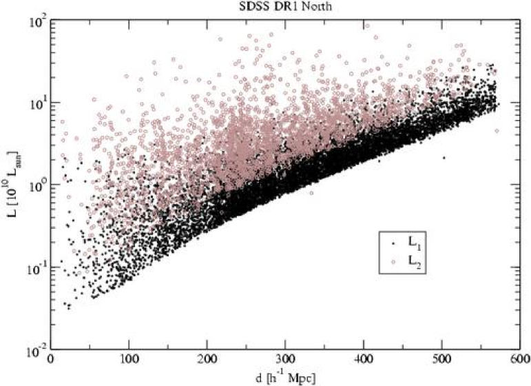
Figure 2: The luminosities of SDSS Northern groups/clusters at different distances, corrected for galaxies outside the visibility window. Grey symbols stand for groups with at least two visible galaxies, black symbols – for groups containing only one galaxy in the visibility window. The luminosity dependence of galaxies of the SDSS Southern slice is very close to that of the Northern slice.

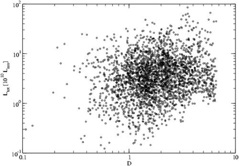
Figure 3: The luminosities of the SDSS DR1 Northern slice clusters as a function of the environmental density, found by Gaussian smoothing of the luminous density field with the rms scale 10 $h^{-1}$ Mpc. Data for the Southern slice are very similar.

3.2 Properties of the SDSS clusters in various environments

Fig. 2 shows the luminosities of groups/clusters at different distances from the observer. We see that there exists a well-defined lower limit of cluster luminosities at larger distances. The limit is linear in the $\log L-d$ plot. Such behavior is expected as at large distances an increasing fraction of clusters do not contain any galaxies bright enough to fall into the observational window of absolute magnitudes, $M_{1}\dots M_{2}$. The limit is lower for groups containing only one galaxy in the visibility window; these groups are systems like our Local group with one bright galaxy surrounded by faint companions. The difference in the low-luminosity limits of groups containing at least one or two galaxies in the visibility window is by a factor of two as expected (this factor corresponds to the case when two galaxies in the visibility window have the same luminosity).

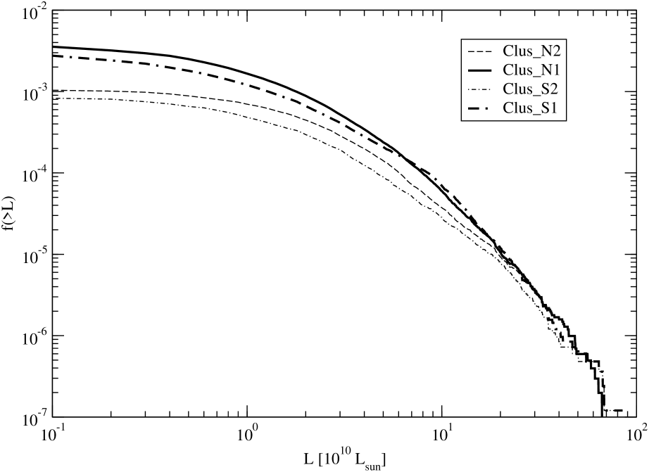
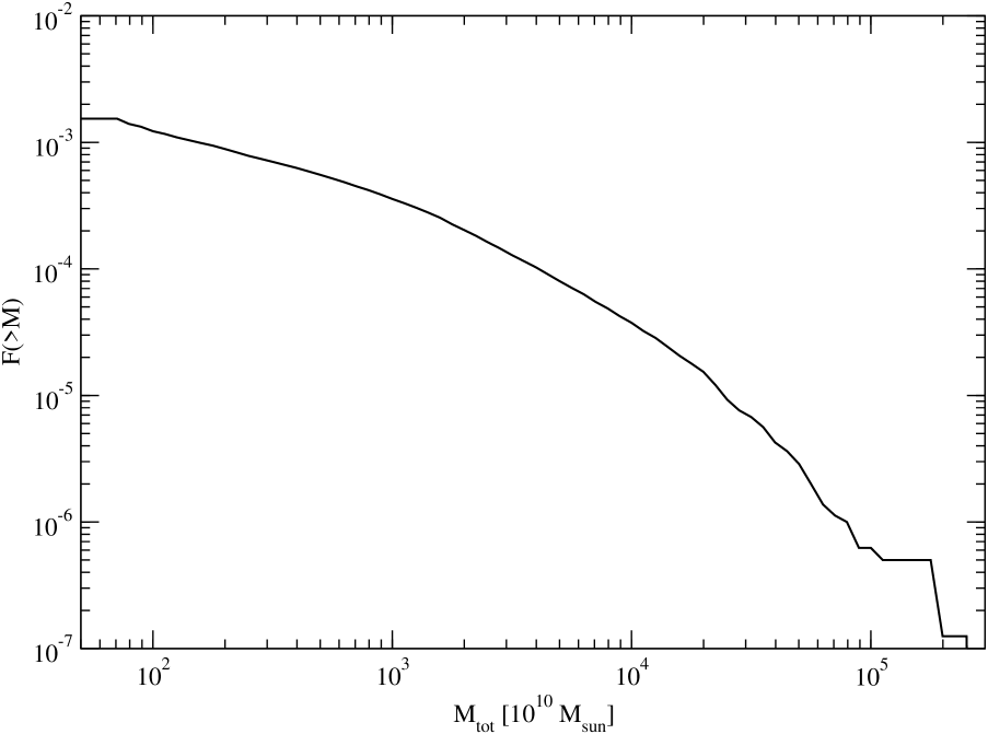
Figure 4: Left: the luminosity functions of the SDSS DR1 groups/clusters. Thin lines show the luminosity functions found using the clusters with at least two galaxies in the observational window, bold lines show luminosity functions for all groups/clusters, including groups with only one galaxy in the observational window. When calculating the total luminosities of groups, the Schechter function parameters of the set E1 were used. Right: the cumulative function of the total masses of DM-haloes of the model M200B.

Let us compare now properties of groups/clusters in various environments. We shall use the density found with the 10 $h^{-1}$ Mpc smoothing as the global density in the supercluster environment of clusters. The environmental effect is shown in Fig. 3. There is a correlation between the luminosity of the most luminous clusters and their environmental density. The most luminous clusters in high-density regions have a luminosity a factor of about 5 higher than the most luminous clusters in low-density regions. Using a different definition of the large-scale environment, a similar effect was found in the vicinity rich clusters of galaxies by E03c and E03d, and in the vicinity of massive DM-halos by E04b.

3.3 Cluster luminosity functions

Fig. 4 shows the integrated luminosity functions of the groups/clusters of the SDSS DR1 Northern and Southern samples. The absence of low-luminosity clusters at large distances has been taken into account by the standard $V_{max}^{-1}$ weighting procedure (for details see E03a). The luminosity function was calculated separately for groups/clusters with at least two visible galaxies, and for all groups/clusters including the systems with only one visible galaxy in the visibility window. In both cases the numbers of clusters have been corrected for selection effects. We see that in the second case the number of groups/clusters per unit volume is larger by a factor of $\sim$3 for the low luminosity section of the luminosity function. This result shows that the groups with one bright main galaxy dominate among low-luminosity groups. We believe that this higher density represents the true number-density of low-luminosity groups better than the density found from groups with at least two galaxies in the observational window. It is well known that in our vicinity the majority of groups are similar to our Local Group, which consists of two subgroups with one bright main galaxy (our Galaxy and M31) and a number of considerably fainter companion galaxies.

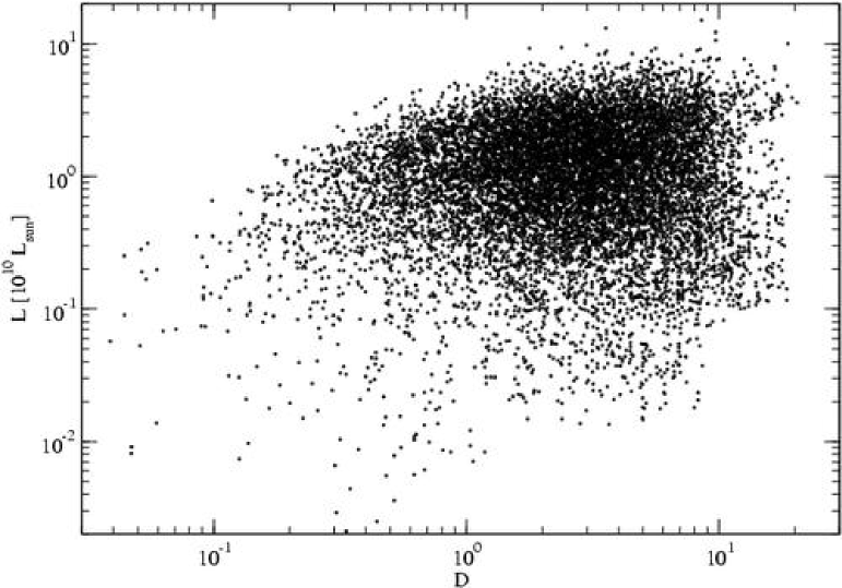
Figure 5: The luminosities of galaxies in various density environments for the SDSS EDR Southern slice. The environmental density was calculated using Gaussian smoothing with the rms scale of 2 $h^{-1}$ Mpc.

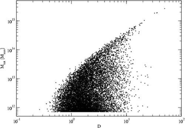
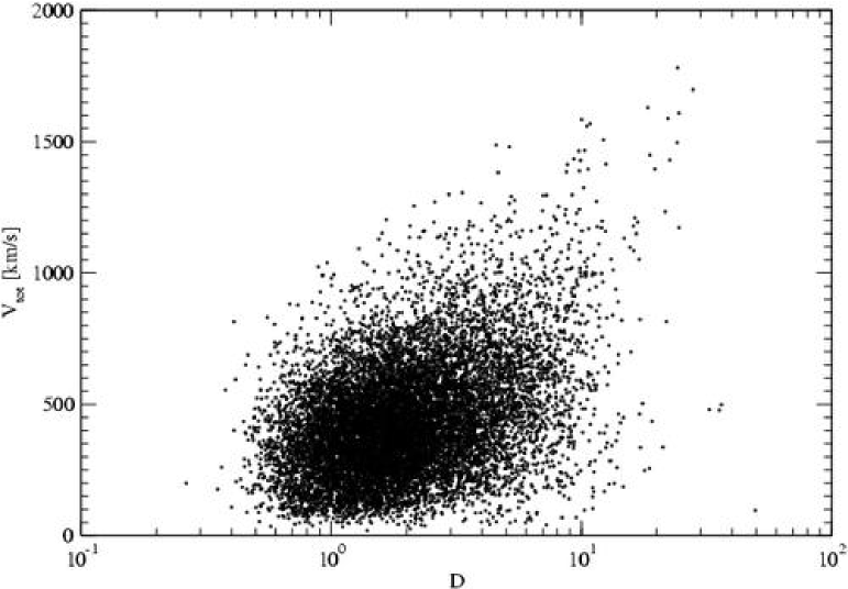
Figure 6: The dependence of the parameters of DM-haloes in the model M200B on the density of the environment, $D$ (in units of the mean density). The density of the environment was determined from the low-resolution field using the Epanechnikov kernel with a radius of 8 $h^{-1}$ Mpc. Left panel: total mass; right panel: full velocity.

3.4 Luminosities of galaxies in different environments

It is well known that in clusters brighter galaxies are concentrated toward cluster centres. For this reason the smoothing scale must be relatively small in order to be sensitive to the positions of galaxies within clusters. Taking this into account we shall use the density found with the 2 $h^{-1}$ Mpc smoothing as an environmental parameter to describe the surrounding density of galaxies. The luminosity of galaxies as a function of the environmental density is shown in Fig. 5; here we used the SDSS EDR to calculate the luminosity density. This figure shows that the most luminous galaxies in high-density regions are about 5–10 times more luminous than the most luminous galaxies in low-density environments. It is interesting that the contrast in luminosity between the high- and low-density regions is of the same order than the luminosity contrast of groups/clusters between the high- and low-density regions.

4 Clusters in simulations

4.1 DM haloes and density fields

The second goal of our study is comparison of observational data with numerical simulations. We have used for this purpose three simulations, M100, M200A and M200B, with $128^{3}$ and $256^{3}$ particles in 100 $h^{-1}$ Mpc and 200 $h^{-1}$ Mpc cubes, respectively. The cosmological parameters of the models are given in Table 2. In the analysis that follows we used the DM-haloes identified by the FoF algorithm with the search radius 0.23 (in units of the mean particle separation) for the model M200B.

The density fields for the N-body simulations were found using all particles of simulations, i.e. we calculated the simulated true total matter density fields. The high-resolution density was found using the conventional cloud-in-cell (CIC) scheme and additional Gaussian smoothing with the rms scale 0.8 in grid cell units (0.6 $h^{-1}$ Mpc). Gaussian smoothing was used in order to avoid the presence of numerous empty cells in low-density regions. The low-resolution density field was calculated using an Epanechnikov kernel with the radius 10 in grid units, which corresponds to 8 $h^{-1}$ Mpc. This field was applied to find simulated superclusters and environmental densities of DM-haloes.

Table 3: The threshold density, volume and mean density of various environments

Sample Threshold Volume Density

$$D_{0}$$ Void P fil R fil Scl Void P fil R fil Scl

0.706 0.845 1.035 17.3 20.8 27.1 34.8 0.548 0.732 0.929 1.442

0.587 0.828 1.239 25.8 24.8 26.3 23.0 0.374 0.619 0.955 2.166

0.527 0.857 1.552 32.8 26.9 24.4 15.9 0.289 0.566 1.035 3.151

0.484 1.000 2.661 46.7 26.7 19.1 7.5 0.207 0.549 1.350 6.641

4.2 Properties of DM-haloes in different environments

The dependence of the total mass of DM-haloes on the density of the environment is shown in the left panel of Fig. 6. Here the dependence of the DM-halo mass on the density of the environment is very well expressed: the most massive clusters in a high-density environment are by a factor of a hundred more massive than the most massive clusters in a low-density environment. For a numerical simulation, we have also information on the velocities of DM-haloes, which is absent for the SDSS DR1 groups/clusters. The right panel of Fig.  6 shows the dependence of the full cluster velocity on the density of the environment. The full velocity has a less pronounced density dependence, but here, too, DM-haloes in most dense environments have a factor of ten larger velocities than DM-haloes in less dense environments.

A similar result was obtained by E04b using a different definition of the density of the environment (the distance to the 5th nearest neighbour). In this paper, in addition to the correlations considered here, the virial radii and the intrinsic rms velocities of DM-haloes in various environments were also studied. The virial radii of DM-haloes in a high-density environment are larger than those in a in low-density environment, but here the contrast between the high- and low-density regions is not so large. The rms velocities of DM-haloes have a very strong environmental dependence, similar to the dependence observed for masses. This is natural, as the rms velocities of virialized haloes are determined by their masses.

5 The evolution of various environmental regions

To understand better the dependence of cluster properties on the environment we determined the distribution of particle densities in regions of various environmental density. For this purpose, for the model M200A we found for every particle in the simulation two density values, the local and the global density. The local density attributed to the particle was found as described above with Gaussian smoothing with the rms scale 0.8 in grid cell units (0.6 $h^{-1}$ Mpc). The global density was found using the low-resolution density field as described above (smoothed with the Epanechnikov kernel of the radius 8 $h^{-1}$ Mpc). The density fields and particle densities were found for four epochs of the simulation, corresponding to the redshifts $z=5,\leavevmode\nobreak\ 2,\leavevmode\nobreak\ 1,\leavevmode\nobreak\ 0$. The simulations started at the redshift $z=50$, so at all epochs considered in our analysis the density field was well evolved.

We divided the whole simulation volume into four regions by increasing global density. These regions correspond to voids, poor and rich filaments, and superclusters. The analysis of the distribution of particles for the present epoch $z=0$ shows that approximately 50%  of all particles are presently located in rich supercluster regions with the global density $D>2.661$. Rich filaments (actually poor superclusters) can be localised as systems lying in the range of global densities $1<D\leq 2.661$; at the present epoch about 25% of particles lie in this density range. Poor filaments can be found as systems in the global density range $0.484<D\leq 1$; about 15 % of particles lie presently in this density range. The rest of particles at global densities $D\leq 0.484$ constitute the void region; the fraction of particles in this density range is at the present epoch about 10%.

If we are interested in the dynamics of different individual regions we have to trace back the positions of individual particles. This approach has been followed by Gottlöber et al. (gottl03 (2003)) in their study of the evolution of individual voids. Our task is simpler, as we are interested in the evolution of the simulation sample as a whole. It is clear that during the evolution DM-particles cluster locally to form DM-haloes, but most particles do not change their large-scale environment. The larger the scale, the smaller are the velocities at that scale. In other words, we may assume that the same fraction of particles presently located in the region of the highest global density was in earlier epochs also in the regions of the highest global density, and similarly the fractions of particles in other ranges of global density did not change. Under this assumption we found for each simulation epoch threshold global densities $D_{i}$ which divide the sample of all particles at a given epoch into regions of global density which occupy, from lowest values upward, 10%, 15%, 25%, and 50% of all particles. As noted above, we call the respective regions the void regions, the poor and rich filament regions, and the supercluster regions. The respective global density thresholds for all epochs considered are given in Table 3.

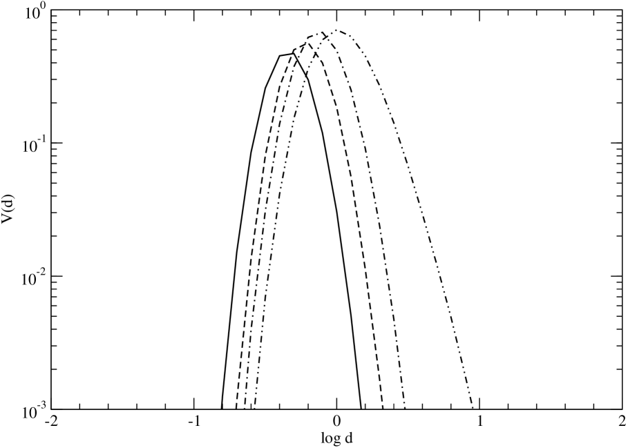
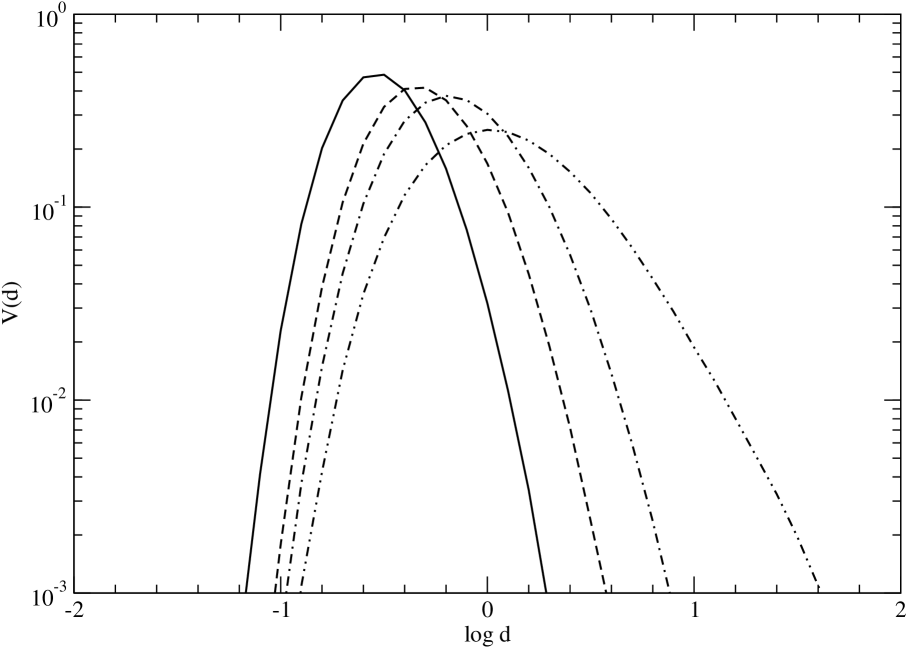
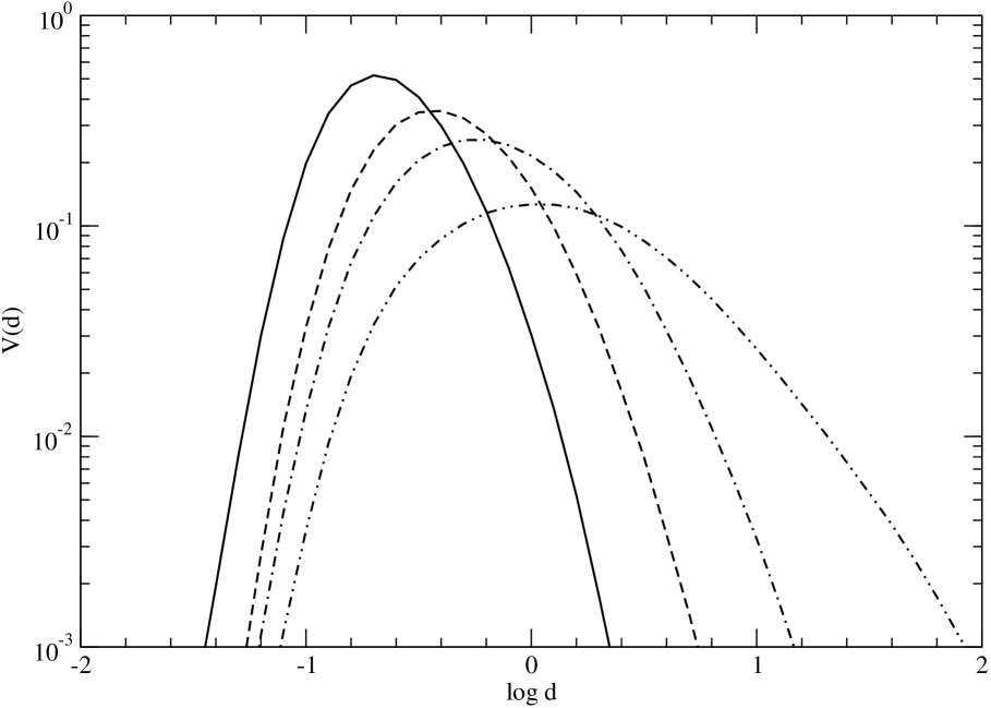
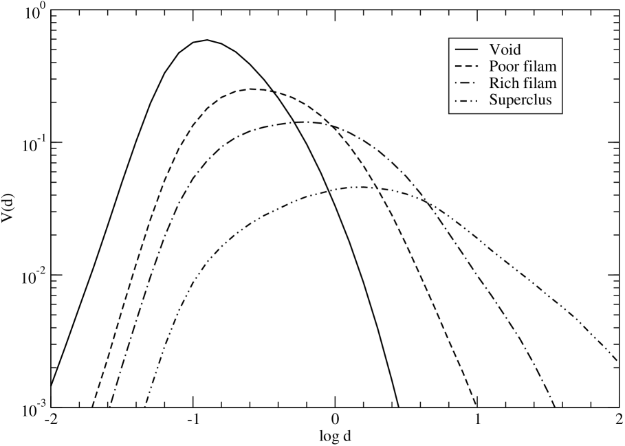
Figure 7: The distribution of volume fraction as a function of local density $d$ in regions of various environment in model M200A. The distribution is found for various regions of global density which correspond to voids, poor and rich filaments, and superclusters, containing 10%, 15%, 25%, and 50% of all particles in regions of increasing global density $D$, respectively. The upper panels are for the epochs $z=5$, and $z=2$, and the lower panels for the epochs $z=1$ and $z=0$ (from left to right).

During their dynamical evolution, superclusters shrink in volume and voids expand. To follow the change of the volume of various environmental regions we give in Table 3 the volume occupied by various regions (in per cents of the total simulation volume). The distribution of volume fraction as a function of the local density $d$ is shown in Fig. 7, for all epochs of simulation. Different lines show the distribution for various global density $D$ ranges: the void, the poor and rich filament, and the supercluster range. The fraction of particles in each region is known, so we can calculate the mean density of matter in each region (in units of the overall mean density); these mean densities are also given in the table. We see that void regions occupy initially (at $z=5$) only 17% of the volume, during evolution this fraction grows to 47%, and the mean density shrinks from 0.5 to 0.2. Fig. 7 shows that in lowest density regions the density is at present epoch less than 0.01. On the other hand, the 50% of all matter that lies in high-density regions (superclusters) occupies initially 35% of space, this fraction decreases to 8%, and respectively the mean density increases from 1.4 to 6.6; in the highest density regions it is higher than 100. The poor and rich filament regions have intermediate behaviour, their volume fractions and mean densities changing much less.

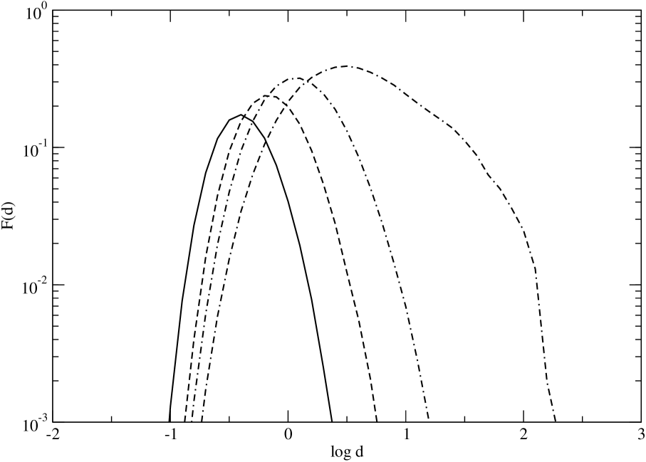
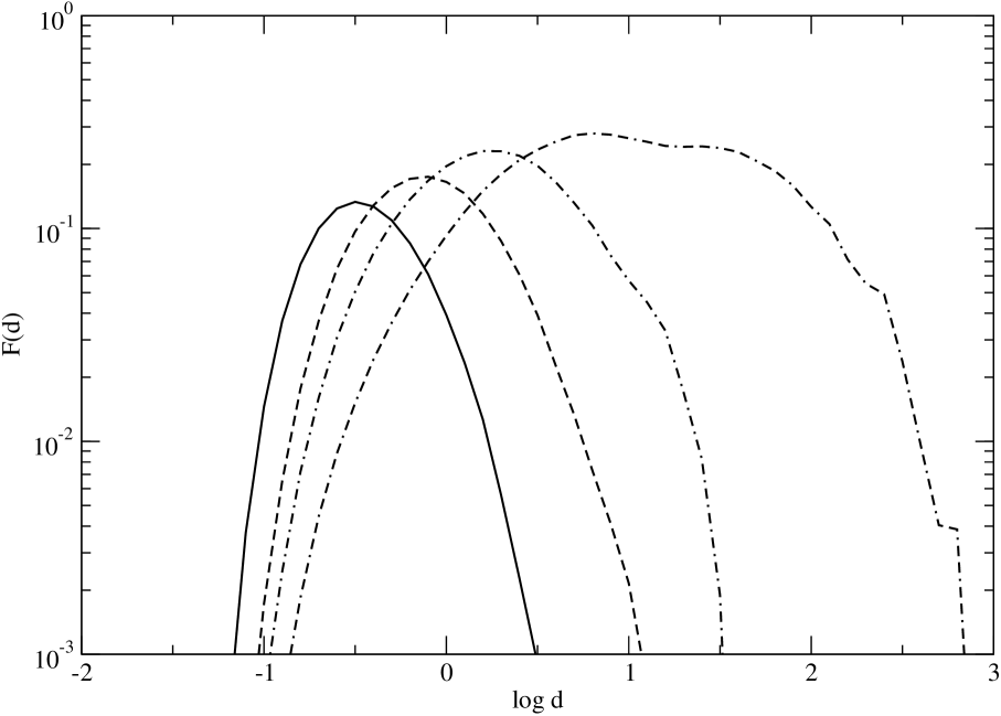
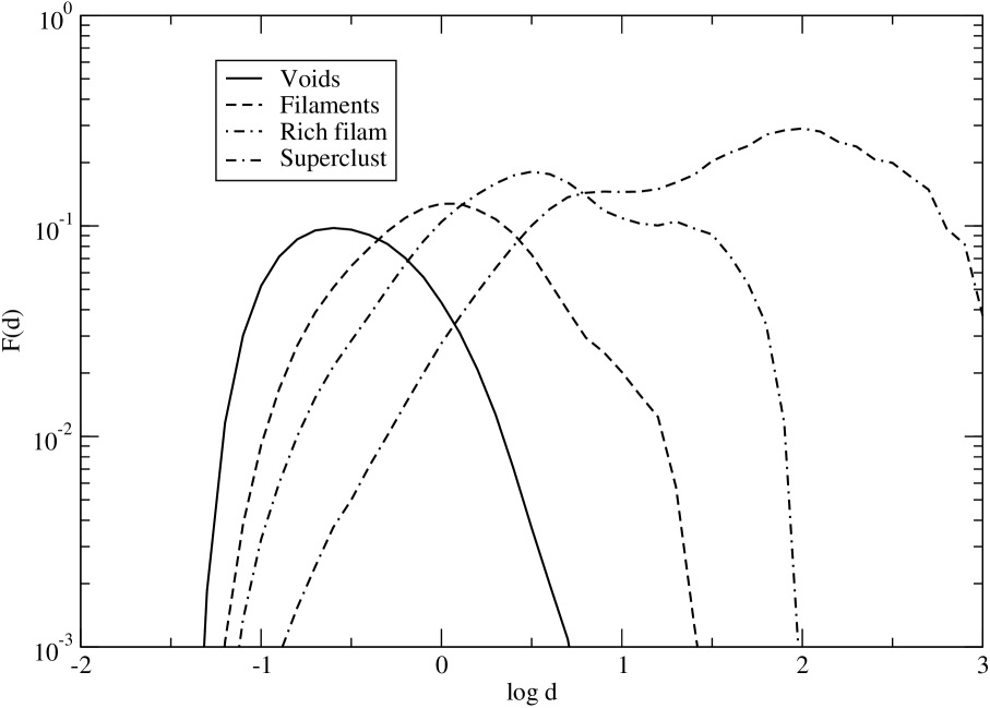
Figure 8: The distribution of particles as a function of local density $d$ in regions of various environment in the model M200A. The distribution has been found for various regions of global density which correspond to voids, poor and rich filaments, and superclusters, containing 10%, 15%, 25%, and 50% of all particles in regions of increasing global density $D$, respectively. The upper panels show the epochs $z=5$, and $z=2$, and the lower panels show the epochs $z=1$ and $z=0$ (from left to right).

Table 4: The fraction of particles of various local density in different environments

Sample Voids Poor filaments Rich filaments Superclusters

0 1 2 0 1 2 0 1 2 0 1 2

$$z=5$$ 8.4 1.1 0.0 10.4 4.8 0.0 11.6 13.5 0.0 8.9 40.1 1.1

8.3 1.4 0.0 8.8 6.5 0.1 8.1 16.1 1.0 4.8 26.4 18.7

7.9 1.6 0.0 7.4 7.4 0.4 5.8 15.3 4.2 2.6 16.8 30.7

7.4 2.2 0.0 5.0 8.1 1.5 3.0 12.9 9.9 0.8 8.8 40.3

We determined in each of the regions the distribution of the particles by their local density $d$. Using the local density, we can assign particles to different populations. We emphasize that particles with local densities less than 1 cannot belong to clusters or groups, since galaxy formation starts only when the local density exceeds a certain critical threshold much higher than the mean density (see Press & Schechter ps74 (1974)). Following these ideas we classify the population of particles with local density below unity as primordial (non-clustered) particles, the population of particles with the local density values in the range $1\leq d<10$ as poor cluster (group) particles, and the population of particles with the local density values $d>10$ as rich cluster particles. For an illustration of the distribution of particles of populations with various local densities see Fig. 1 of Einasto et al. (1999ApJ…519..456E (1999)).

The distribution of the number of particles according to their local density $d$ is given in Fig. 8 for all simulation epochs considered. The Figure is similar to the previous one, only here we plot the distribution of mass instead of volume. The Table 4 gives the fractions of particles (in per cents of the total number of particles in simulation), which belong to populations of various local density: the populations of the primordial, the poor cluster and the rich cluster particles; these populations are denoted as 0, 1 and 2, respectively. The fractions are given, as explained above, separately for the void, the poor filament, the rich filament, and the supercluster environment.

Let us discuss the data in more detail. Consider, first, the void regions. The void particle population distributions are drawn in Figs. 7 and  8 by solid lines (see also the columns labeled 0 in Table 4). We see that at all epochs the distribution of local densities of void particles is rather symmetrical, both in volume and mass. In void regions most particles belong at all epochs to the primordial non-clustered population 0. At the epoch $z=5$ about 1% of the particles belong to the poor cluster population (the columns labeled 1 in Table 4); this fraction increases with time and reaches 2.2% at the present epoch ($z=0$). Initially there are no particles of rich cluster population among void particles (columns 2), and at the present epoch a very tiny fraction of particles has crossed the threshold of the rich cluster population.

The distribution of particles in the poor filament regions is plotted in Figs. 7 and  8 by dashed lines. We see that the initial distribution of particles is similar to the distribution in void regions; however, the distributions are shifted toward higher local density values, and thus the fraction of the poor cluster population 1 is higher. The poor cluster population 1 grows with time, so that at the present epoch about half of the poor filament particles belong to it. The rich cluster population 2 fraction in these regions grows from zero to 1.5%. Most of the volume in the poor filament region is occupied by local voids with local density values $d<1$ (see Fig. 7).

The evolution of particles in the rich filament environment is shown in Figs. 7 and  8 by dot-dashed lines. In this region initially about half of the particles belong to the primordial population 0, and the other half to the poor cluster population 1; there are no particles of the rich cluster population 2. As time goes by, the fraction of primordial particles rapidly decreases and the fraction of rich cluster particles increases; the fraction of poor cluster particles changes little.

For the evolution of the supercluster region see the dot-dash-dashed lines in Figs. 7 and  8. In this environment the fraction of primordial particles 0 rapidly decreases with time to almost zero, the fraction of poor cluster particles 1 decreases from about 40% to 9%, and the fraction of rich cluster population 2 increases from 1% to 40% (from $z=5$ to $z=0$). A large fraction of particles have local densities far in excess of our limiting density $d=10$. However, a considerable fraction of space is still occupied by local voids, as seen from Fig. 7.

These results can be summarized as follows: in void regions the mean density decreases continuously, as a result DM-haloes almost do not evolve dynamically, and most particles remain as primordial (non-clustered) ones. In supercluster regions the dynamical evolution is very rapid, the primordial population clusters rapidly, and later evolution consists of the transition of galaxies and groups to rich clusters. Here we have not followed the evolution of individual clusters, but it is clear that in this later stage merging of smaller DM-haloes to form rich DM-haloes plays an important role. In poor and rich filament regions the evolution is between these two extreme cases.

6 Discussion

6.1 Luminosity/mass functions in real and simulated clusters

Let us compare first the luminosity and mass functions of real and simulated groups/clusters. In our preliminary study (E03a and E03b) we defined groups and clusters as enhancements of the 2-dimensional high-resolution luminosity density field. In the present work we used full 3-dimensional data to define groups/clusters, both for the real data and simulations.

New more accurate data show (see Fig. 4), that there is no essential difference between the luminosity functions in the Northern and Southern strip of the survey. Our preliminary analysis based on the SDSS EDR and groups/clusters defined using the 2-dimensional luminosity density data suggested the presence of differences between the Northern and Southern strips. The new analysis does not support our previous conclusion.

The volume density of groups/clusters according to the SDSS DR1 data is $3\times 10^{-3}$ ($h^{-1}$ Mpc)^-3 for $L\geq 10^{9}$ $L_{\odot}$ groups/clusters. This estimate is in fairly good agreement with the estimates of the number density of groups based on the group mass function by Girardi & Giuricin (gg00 (2000)), see also Heinämäki et al. (hei03 (2003)).

The luminosity of simulated DM-haloes is not well-defined. Thus we use for comparison the integrated mass function of DM-haloes in simulations, presented in the right panel of Fig. 4. We see that the overall shape of the integrated mass function is rather similar to the luminosity function of the real groups/clusters. In the low-mass range the mass function of DM-haloes is steeper than the luminosity function of the real groups/clusters. The presently available data are insufficient to judge if this difference is significant or not; a more detailed study of simulated samples is needed, with simulated galaxies generated in DM-haloes. The mean volume density of DM-haloes is very close to the mean volume density of groups in the SDSS DR1, thus we can say that the population of DM-haloes represents the population of real groups/clusters rather well (the overall bias is small).

6.2 Environmental effects in real and simulated clusters

Let us compare now the environmental dependence in real and simulated cluster samples. The environmental dependence has been investigated using two completely independent parameters to characterize the large-scale environment. E03c compared groups and clusters in high density environments, defined as a neighbourhood of rich clusters, and in low density environments, far from rich clusters. E03d compared the properties of groups and clusters that belong to superclusters and the properties of groups/clusters that do not belong to superclusters. E04b used the distance to the 5th nearest neighbour as a parameter of the large-scale environment to describe the environment of DM-haloes in simulations. E03a and E03b used for this purpose the low-resolution luminosity density field, as we do in the present study.

These parameters of the large-scale environment used in various studies are independent of each other and characterize the environment from different points of view. The luminosity density field approach takes into account the luminosity or the mass of neighbouring objects, including the dark matter particles in simulations. The nearest neighbour approach, as well as the proximity to rich clusters, depends only on the number and position of neighbours. Their luminosity or mass is ignored.

All relations considered so far between the physical parameters of groups/clusters and the environmental parameter show the presence of well-defined correlations, both in real as well as in simulated samples: in high-density regions (superclusters) groups/clusters are brighter and more massive than in low-density regions (void regions). Also they have slightly larger radii and greater bulk velocities (see E04b).

6.3 Comparison to previous work

Historically, the dependence of galaxy properties on their large-scale environment has been investigated long ago, starting from the pioneering studies by Davis & Geller (dg76 (1976)) and Dressler (dr80 (1980)). In these early studies a striking contrast between the morphological types of galaxies in the cluster and field environments was found: in clusters elliptical galaxies dominate and in the field dominate spiral and irregular ones. More recently Einasto (1991a , 1991b ) and Mo et al. (mexd92 (1992)) found the dependence of galaxy luminosity and morphological type on the large-scale environment up to the scale of 10 $h^{-1}$ Mpc. This result was confirmed by Lindner et al. (l95 (1995),  l96 (1996)) by the study of voids defined by galaxies of different absolute magnitude: bright galaxies define much larger voids than intrinsically faint galaxies; these faint galaxies form poor filaments inside large voids surrounded by bright galaxies.

Recently Balogh et al. (balogh04 (2004)), and Blanton et al. (2004a , 2004b , see also references in these papers) investigated the dependence of physical properties of galaxies in different local and global environment. Among physical properties they considered colours, luminosities, H$\alpha$ emission, and the Sérsic (sersic68 (1968)) luminosity radial profile index. The local environment was defined as the spatial density on the 0.5–1 $h^{-1}$ Mpc scale, the global density on the 5–10 $h^{-1}$ Mpc scale. Blanton et al. (2004b ) come to the conclusion that the blue galaxy fraction, and the recent star formation history in general, depend mostly on the local environment. On the other hand, Croton et al. (cr04 (2004)) find that the luminosity function of galaxies depends strongly on the global environment (see below).

Peebles (p01 (2001)) compared void and cluster galaxies and confirmed the presence of a striking difference of the properties of these galaxies. He argued that this difference may be a challenge to the $\Lambda$CDM model of structure formation. Mo et al. (mo04 (2004)) came to the conclusion that the differences in luminosity observed in regions of different environmental density can be attributed to the differences in the mass of DM-haloes from which galaxies form. As our present study shows, the masses themselves depend on the environment.

The luminosity dependence of galaxy clustering was investigated by Norberg et al. (n01 (2001), n02 (2002)), using the 2dF Galaxy Redshift Survey. They found that the clustering amplitude increases with absolute magnitude, confirming earlier results by Einasto, Klypin & Saar (eks86 (1986)), Bromley et al. (bplk98 (1998)), and Beisbart & Kerscher (bk00 (2000)).

The luminosity function of galaxies in different environment was recently investigated by Hütsi et al. (h02 (2002)), De Propris et al. (dp03 (2003)) and Mo et al. (mo04 (2004)). Hütsi et al. estimated the luminosity function in three regions of global density, defined by the 10 $h^{-1}$ Mpc smoothing, and found that the characteristic luminosity of galaxies increases by a factor of 1.5 from the low-density to the high-density regions. Mo et al. argued that this difference in the characteristic luminosity is in agreement with their model prediction, which assumes that the Schechter approximation is valid in virtually all environments.

A very detailed study of luminosity functions of galaxies in regions of different density of the large-scale environment was made by Croton et al. (cr04 (2004)), using the full dataset of the 2dF Galaxy Redshift Survey. Using densities smoothed on a scale of 8 $h^{-1}$ Mpc  as in the present paper, he divided the volume under study into 7 regions of various density of the environment, from extreme void to cluster populations. In all regions the luminosity function was calculated and the parameters of the Schechter function were found. The bright end of the function depends primarily on the characteristic absolute magnitude $M^{*}$ of the Schechter function. For the extreme void population this parameter is $-18.3$, and for the cluster population $-20.1$. In other words, the brightest galaxies in voids are approximately 5 times fainter than in clusters. This result is in very good agreement with our data on the distribution of galaxy luminosities of the SDSS in various environments (see Fig. 5).

The dependence of the total luminosities and masses of galaxy systems on the density of the environment has been investigated only recently by E03a, E03b, E03c, E03d, E04a and E04b (for a discussion about the properties of haloes in different environments see references in this paper). These studies show a tendency similar to that of galaxy luminosities – in high-density regions massive and luminous clusters dominate, whereas in low-density regions all galaxy systems are poor and faint. The most luminous clusters in a high-density environment are a factor of 5–10 more luminous than the most luminous clusters in a low-density environment. It is striking that this factor is in the same range as for the most luminous galaxies in high- and low-density environments.

The properties of groups of galaxies in the vicinity of rich clusters were compared with the properties of ordinary groups by Ragone et al. (ragone04 (2004)). They used a sample of groups identified in the 2dF Galaxy Redshift Survey, and compared the properties of groups in the vicinity of rich clusters and the rest of the sample. The observational results were compared with simulated clusters using the Virgo Consortium Simulation. In both the real and simulated groups there exist similar relations: the larger the host mass, the higher is the luminosity or the mass of the DM-halo.

Comparison of the richness of DM-haloes in different environments was made by Gottlöber et al. (gottl03 (2003)), using high-resolution numerical simulations. Their results show that DM-haloes in voids have much lower masses than in high-density environments. This result was recently confirmed by Colberg et al. (colberg04 (2004)). Their Fig. 14 demonstrates that the most massive DM-haloes in voids are about 100 times less massive than the most massive DM-haloes in general; also the growth of masses of DM-haloes in voids is less rapid than in general.

6.4 Interpretation of the environmental dependence of galaxy and cluster properties

One may ask, why are void galaxies and clusters so different from galaxies and clusters in dense regions?

The evolution of DM-haloes in numerical simulations has been investigated by a number of authors. Several of these simulations have been visualized, as an example those by Andrey Kravtsov (http://cfcp.uchicago.edu/lss/filaments.html). In this simulation the formation of rich clusters and superclusters consisting of a system of intertwined filaments can be clearly seen.

We are interested in the difference between the structure of galaxy systems in high- and low-density environments. This problem has been studied in detail by Gottlöber et al. (gottl03 (2003), for earlier work see references in this paper). They chose several large under-dense regions of a diameter of $\sim$20 $h^{-1}$ Mpc (voids defined by bright simulated galaxies) and re-simulated the evolution of these voids with a very high mass resolution $4.0\times 10^{7}\leavevmode\nobreak\ h^{-1}M_{\odot}$. Their Fig. 2 shows the distribution of dark matter in one of these voids at the epochs $z=2$ and $z=0$. At both epochs a well-developed system of filaments with compact knots (DM-haloes) can be seen. However, the masses of these haloes are at both epochs of the order of $10^{9}\leavevmode\nobreak\ h^{-1}M_{\odot}$, only the most massive ones have masses of few times of $10^{10}\leavevmode\nobreak\ h^{-1}M_{\odot}$. In other words, after the early growth the knots stop growing. The volume density of DM-haloes in these voids is a factor of 10 lower that in the simulation as a whole.

In contrast, the growth of DM-haloes in high-density regions is much more rapid and continues over the whole period under study. As shown, among others, by Frisch et al. (f95 (1995)), the first objects to form in simulations are rich clusters in superclusters. Our calculations presented in the last Section fully confirm these earlier conclusions.

7 Conclusions

The main results of our study of clusters and superclusters in the SDSS DR1 and the comparison with the results of numerical simulations can be summarised as follows:

• We have found groups and clusters in the SDSS DR1 data using three-dimensional information on the distribution of galaxies.

• Using Gaussian smoothing with the rms scales of 0.8 and 10 $h^{-1}$ Mpc we have derived high- and low-resolution luminosity density fields for the SDSS DR1 data in two equatorial strips; the low-resolution density was used as an environmental parameter to describe the large-scale environment of groups and clusters.

• New three-dimensional data confirm the environmental dependence found earlier using the two-dimensional data: in high-density regions (superclusters) groups and clusters are richer and bigger, and galaxies themselves are brighter.

• Numerical simulations show a similar tendency: in a high-density environment DM-haloes are richer, and have larger bulk motions than DM-haloes in a low-density environment.

• Our explanation of the density-luminosity relationship is by the combined influence of density perturbations of all scales. Superclusters are the regions where the density perturbations of large and medium wavelength combine to generate high-density peaks: here the overall density is high and the dynamical evolution of clusters and galaxies is rapid and continues until the present. Voids are regions where large-scale density perturbations have negative amplitudes; here, due to medium and small-scale perturbations also a filamentary web forms; however, due to the low mean density the dynamical evolution is slow and stops at an early epoch.

- (1) Abazajian, K., Adelman-McCarthy, J. K., Agüeros, M. A., et al. 2003, AJ, 126, 2081
- (2) Abell, G. 1958, ApJS, 3, 211
- (3) Abell, G., Corwin, H., & Olowin, R. 1989, ApJS, 70, 1
- (4) Balogh, M., Eke, V., Miller, C., et al. 2004, MNRAS, 348, 1355, astro-ph/0311379
- (5) Beisbart, C., & Kerscher, M. 2000, ApJ, 545, 6
- (6) Bennett, C. L., Hill, R. S., Hinshaw, G., et al., 2003, ApJS, 148, 119
- (7) Blanton, M. R., Dalcanton, J., Eisenstein, D. et al. 2001, AJ, 121, 2358
- (8) Blanton, M.R., Eisenstein, D., Hogg, D.W., et al. 2004a, ApJ (accepted), astro-ph/0310453
- (9) Blanton, M.R., Eisenstein, D., Hogg, D.W., et al. 2004b, ApJ (submitted), astro-ph/0411037
- (10) Bromley, B.J., Press, W.H., Lin, H., et al. 1998, ApJ, 505, 25
- (11) Colberg, J.M., Sheth, R.K., Diaferio, A., Gao, L., et al. 2004, MNRAS, (in press), astro-ph/0409162
- (12) Croton, D.J., Farrar, G. R., Norberg, P. et al. 2004, MNRAS (accepted), astro-ph/0407537
- (13) Davis, M., & Geller, M.J. 1976, ApJ, 208, 13
- (14) De Propris, R., Colless, M., Driver, S.P., et al. 2003, MNRAS, 342, 725
- (15) Dressler, A. 1980, ApJ, 236, 351
- (16) Einasto, J., Einasto, M., Hütsi, G., et al. 2003a, A&A, 410, 425, (E03a)
- (17) Einasto, J., Einasto, M., Tago, E., et al. 1999, ApJ, 519, 456
- (18) Einasto, J., Hütsi, G., Einasto, M., et al. 2003b, A&A, 405, 425, (E03b)
- (19) Einasto, J., Tago, E., Einasto, M., & Saar, E. 2004a, ”Nearby Large-Scale Structures and the Zone of Avoidance”, Cape Town, 28 March - 02 April 2004, eds. A. Fairall & P. Woudt, astro-ph/0408463 (E04a)
- (20) Einasto, J., Klypin, A.A. & Saar, E. 1986, MNRAS, 219, 457
- (21) Einasto, M. 1991a, MNRAS, 250, 802
- (22) Einasto, M. 1991b, MNRAS, 252, 261
- (23) Einasto, M., Einasto, J., Müller, V., Heinämäki, P.,& Tucker, D. L. 2003c, A&A, 401, 851, (E03c)
- (24) Einasto, M., Jaaniste, J., Einasto, J., et al. 2003d, A&A, 405, 821, (E03d)
- (25) Einasto M., Suhhonenko, I., Heinämäki, P., & Einasto J. 2004b, A&A, (in preparation, E04b)
- (26) Frisch, P., Einasto, J., Einasto, M., et al. 1995, å, 296, 611
- (27) Girardi, M., & Giuricin, G. 2000, ApJ, 540, 45
- (28) Gottlöber, S., Lokas, E. L., Klypin, A., et al. 2003, MNRAS, 344, 715
- (29) Heinämäki, P., Einasto, J., Einasto, M., et al. 2003, A&A, 397, 63
- (30) Huchra, J. P., & Geller, M. J. ApJ, 257, 423
- (31) Hütsi, G., Einasto, J., Tucker, D.L. et al. 2002, astro-ph/0212327
- (32) Jenkins, A., Frenk, C.S., White, S.D.M., et al. 2001, MNRAS, 321, 372
- (33) Klypin, A., Holtzman, J., Primack, J., & Regöz, E. 1993, ApJ, 416, 1
- (34) Knebe, A., Green, A. & Binney, J. 2001, MNRAS, 325, 845
- (35) Lindner, U., Einasto, J., Einasto, M., et al. 1995, A&A, 301, 329
- (36) Lindner U., Einasto, M., Einasto, J., et al. 1996, A&A, 314, 1
- (37) Mo, H.J., Einasto, M., Xia, X.Y. & Deng, Z.G. 1992, MNRAS, 255, 382
- (38) Mo, H.J., Yang, X., van den Bosch, F.C., et al. 2004, MNRAS, 349, 205
- (39) Norberg, P., Baugh, C.M., Hawkins, E., et al. 2001, MNRAS, 328, 64
- (40) Norberg, P., Baugh, C.M., Hawkins, E., et al. 2002, MNRAS, 332, 827
- (41) Peacock, J.P. 1999, Cosmological Physics, Cambridge Univ. Press
- (42) Peebles, P.J.E. 2001, ApJ, 557, 495
- (43) Press, W.H. & Schechter, P.L. 1974, ApJ, 187, 425
- (44) Ragone, C.J., Mercháb, M., Muriel, H., et al. 2004, MNRAS in press, astro-ph/0402155
- (45) Schechter, P. 1976, ApJ, 203, 297
- (46) Sérsic, J.L. 1968, Atlas de Galaxias Australes (Cordoba Obs. Astronómico)
- (47) Stoughton, C., Lupton, R. H., Bernardi, M. et al. 2002, AJ, 123, 485
- (48) Tegmark M., Strauss, M.A., Blanton, M.R., et al. 2004, PhRvD, 69, 103501, astro-ph/0310723
- (49) Tucker, D.L., Oemler, A.Jr., Hashimoto, Y. et al. 2000, ApJS, 130, 237
- (50) Zeldovich, Ya.B., Einasto, J. & Shandarin, S.F. 1982, Nature, 300, 407
- 1961– (68) Zwicky, F., Wield, P., Herzog, E., Karpowicz, M. & Kowal, C.T. 1961–68, Catalogue of Galaxies and Clusters of Galaxies, 6 volumes. Pasadena, California Inst. Techn.