Modelling the Galaxy for GAIA

Abstract

Techniques for the construction of dynamical Galaxy models should be considered essential infrastructure that should be put in place before GAIA flies. Three possible modelling techniques are discussed. Although one of these seems to have significantly more potential than the other two, at this stage work should be done on all three.

A major effort is needed to decide how to make a model consistent with a catalogue such as that which GAIA will produce. Given the complexity of the problem, it is argued that a hierarchy of models should be constructed, of ever increasing complexity and quality of fit to the data. The potential that resonances and tidal streams have to indicate how a model should be refined is briefly discussed.

1 Introduction

A central goal of the GAIA mission is to teach us how the Galaxy functions and how it was assembled. We can only claim to understand the structure of the Galaxy when we have a dynamical model galaxy that reproduces the data. Therefore the construction of a satisfactory dynamical model is in a sense a primary goal of the GAIA mission, for this model will encapsulate the understanding of galactic structure that we have gleaned from GAIA.

Preliminary working models that are precursors of the final model will also be essential tools as we endeavour to make astrophysical sense of the GAIA catalogue. Consequently, before launch we need to develop a model-building capability, and with it produce dynamical models that reflect fairly fully our current state of knowledge.

2 Current status of Galaxy modelling

The modern era of Galaxy models started in 1980, when the first version of the Bahcall-Soneira model appeared (Bahcall & Soneira 1980). This model broke new ground by assuming that the Galaxy is built up of components like those seen in external galaxies. Earlier work had centred on attempts to infer three-dimensional stellar densities by directly inverting the observed star counts. However, the solutions to the star-count equations are excessively sensitive to errors in the assumed obscuration and the measured magnitudes, so in practice it is essential to use the assumption that our Galaxy is similar to external galaxies to choose between the infinity of statistically equivalent solutions to the star-count equations. Bahcall & Soneira showed that a model inspired by data for external galaxies that had only a dozen or so free parameters could reproduce the available star counts.

Bahcall & Soneira (1980) did not consider kinematic data, but Caldwell & Ostriker (1981) updated the classical work on mass models by fitting largely kinematic data to a mass model that comprised a series of components like those seen in external galaxies. These data included the Oort constants, the tangent-velocity curve, the escape velocity at the Sun and the surface density of the disk near the Sun.

Bienaymé, Robin & Crézé (1987) were the first to fit both kinematic and star-count data to a model of the Galaxy that was inspired by observations of external galaxies. They broke the disk down into seven sub-populations by age. Then they assumed that motion perpendicular to the plane is perfectly decoupled from motion within the plane, and further assumed that as regards vertical motion, each subpopulation is an isothermal component, with the velocity dispersion determined by the observationally determined age-velocity dispersion relation of disk stars. Each sub-population was assumed to form a disk of given functional form, and the thickness of the disk was determined from the approximate formula $\rho(R,z)/\rho(R,0)=\exp\{[\Phi(R,0)-\Phi(R,z)]/\sigma^{2}\}$, where $\Phi$ is an estimate of the overall Galactic potential. Once the thicknesses of the sub-disks have been determined, the mass of the bulge and the parameters of the dark halo were adjusted to ensure continued satisfaction of the constraints on the rotation curve $v_{c}(R)$. Then the overall potential is recalculated, and the disk thicknesses were redetermined in the new potential. This cycle was continued until changes between iterations were small. The procedure was repeated several times, each time with a different dark-matter disk arbitrarily superposed on the observed stellar disks. The geometry and mass of this disk were fixed during the interations of the potential. Star counts were used to discriminate between these dark-matter disks; it turned out that the best fit to the star counts was obtained with negligible mass in the dark-matter disk. Although in its essentials the current ‘Besano̧n model’ (Robin et al. 2003) is unchanged from the original one, many refinements and extensions to have been made. In particular, the current model fits near IR star counts and predicts proper motions and radial velocities. It has a triaxial bulge and a warped, flaring disk. Its big weakness is the assumption of constant velocity dispersions and streaming velocities in the bulge and the stellar halo, and the neglect of the non-axisymmetric component of the Galaxy’s gravitational field.

A consensus that ours is a barred galaxy formed in the early 1990s (Blitz & Spergel 1991; Binney et al. 1991) and models of the bulge/bar started to appear soon after. Binney, Gerhard & Spegel (1997) and Freudenreich (1998) modelled the luminosity density that is implied by the IR data from the COBE mission, while Zhao (1996) and Häfner et al. (2000) used extensions of Schwarzschild’s (1979) modelling technique to produce dynamical models of the bar that predicted proper motions in addition to being compatible with the COBE data. There was an urgent need for such models to understand the data produced by searches for microlensing events in fields near the Galactic centre. The interplay between these data and Galaxy models makes rather a confusing story because it has proved hard to estimate the errors on the optical depth to microlensing in a given field.

The recent work of the Basel group (Bissantz & Gerhard 2002; Bissantz, Englmaier & Gerhard 2003; Bissantz, Debattista & Gerhard 2004) and the microlensing collaborations (Afonso, et al. 2003; Popowski et al. 2004) seems at last to have produced a reasonably coherent picture. Bissantz, Englmaier & Gerhard (2003) fit a model to structures that are seen in the $(l,v)$ diagrams that one constructs from spectral-line observations of HI and CO. The model is based on hydrodynamical simulations of the flow of gas in the gravitational potential of a density model that was fitted to the COBE data (Bissantz & Gerhard 2002). They show that structures observed in the $(l,v)$ plane can be reproduced if three conditions are fulfilled: (a) the pattern speed of the bar is assigned a value that is consistent with the one obtained by Dehnen (2000) from local stellar kinematics; (b) there are four spiral arms (two weak, two strong) and they rotate at a much lower pattern speed; (c) virtually all the mass inside the Sun is assigned to the stars rather than a dark halo.

Bissantz, Debattista & Gerhard (2004) go on to construct a stellar-dynamical model that reproduces the luminosity density inferred by (Bissantz & Gerhard 2002). The model, which has no free parameters, reproduces both (a) the stellar kinematics in windows on the bulge, and (b) the microlensing event timescale distribution determined by the MACHO collaboration (Alcock et al. 2000). The magnitude of the microlensing optical depth towards bulge fields is still controversial, but the latest results agree extremely well with the values predicted by Bissantz & Gerhard: in units of $10^{-6}$, the EROS collaboration report optical depth $\tau_{6}=0.94\pm 0.3$ at $(l,b)=(2.5^{\circ},-4^{\circ})$ (Afonso, et al. 2003) while Bissantz & Gerhard predicted $\tau_{6}=1.2$ at this location; the MACHO collaboration report $\tau_{6}=2.17^{+0.47}_{-0.38}$ at $(l,b)=(1.5^{\circ},-2.68^{\circ})$ (Popowski et al. 2004), while Bissantz & Gerhard predicted $\tau_{6}=2.4$ at this location.

Thus there is now a body of evidence to suggest that the Galaxy’s mass is dominated by stars that can be traced by IR light rather than by invisible objects such as WIMPS, and that dynamical galaxy models can successfully integrate data from the entire spectrum of observational probes of the Milky Way.

3 Where do we go from here?

Since 1980 there has been a steady increase in the extent to which Galaxy models are dynamical. A model must predict stellar velocities if it is to confront proper-motion and radial velocity data, or predict microlensing timescale distributions, and it needs to predict the time-dependent, non-axisymmetric gravitatinal potential in order to confront spectra-line data for HI and CO. Some progress can be made by adopting characteristic velocity dispersions for different stellar populations, but this is a very poor expedient for several reasons. (a) Without a dynamical model, we do not know how the orientation of the velocity ellipsoid changes from place to place. (b) It is not expected that any population will have Gaussian velocity distributions, and a dynamical model is needed to predict how the distributions depart from Gaussianity. (c) An arbitrarily chosen set of velocity distributions at different locations for a given component are guaranteed to be dynamically inconsistent. Therefore it is imperative that we move to fully dynamical galaxy models. The question is simply, what technology is most promising in this connection?

3.1 Schwarzschild modelling

The market for models of external galaxies is currently dominated by models of the type pioneered by Schwarzschild (1979). One guesses the galactic potential and calculates a few thousand judiciously chosen orbits in it, keeping a record of how each orbit contributes to the observables, such as the space density, surface brightness, mean-streaming velocity, or velocity dispersion at a grid of points that covers the galaxy. Then one uses linear or quadratic programming to find non-negative weights $w_{i}$ for each orbit in the library such that the observations are well fitted by a model in which a fraction $w_{i}$ of the total mass is on the $i$th orbit.

Schwarzschild’s technique has been used to construct spherical, axisymmetric and triaxial galaxy models that fit a variety of observational constraints. Thus it is a tried-and-tested technology of great flexibility.

It does have significant drawbacks, however. First the choice of initial conditions from which to calculate orbits is at once important and obscure, especially when the potential has a complex geometry, as the Galactic potential has. Second, different investigators will choose different initial conditions and therefore obtain different orbits even when using the same potential. So there is no straightforward way of comparing the distributon functions of their models. Third, the method is computationally very intensive because large numbers of phase-space locations have to be stored for each of orbit. Finally, predictions of the model are subject to discreteness noise that is larger than one might naively suppose because orbital densities tend to be cusped (and formally singular) at their edges and there is no natural procedure for smoothing out these singularities.

3.2 Torus modelling

In Oxford over a number of years we developed a technique in which orbits are not obtained as the time sequence that results from integration of the equations of motion, but as images under a canonical map of an orbital torus of the isochrone potential. Each orbit is specified by its actions ${\bf J}$ and is represented by the coefficients $S_{{\bf n}}({\bf J}^{\prime})$ that define the function $S({\bf J}^{\prime},\theta)={\bf J}^{\prime}\cdot\theta+\sum_{{\bf n}}S_{\bf n}{\rm e}^{{\rm i}{\bf n}\cdot\theta}$ that generates the map. Once the $S_{\bf n}$ have been determined, analytic expressions are available for ${\bf x}(\theta)$ and ${\bf v}(\theta)$, so one can readily determine the velocity at which the orbit would pass through any given location. Since orbits are labelled by actions, which define a true mapping of phase space, it is straightforward to construct an orbit library by systematically sampling phase space at the nodes of a regular grid of actions ${\bf J}^{\prime}$. Moreover, a good approximation to an arbitrary orbit can be obtained by interpolating the $S_{\bf n}({\bf J}^{\prime})$.

If the orbit library is generated by torus mapping, it is easy to determine the distributon function from the weights. When the orbit weigts are normalized such that $\sum_{i}w_{i}=1$, and the distribution function is normalized such that $\int{\rm d}^{3}{\bf x}{\rm d}^{3}{\bf v}\,f=1$, then

$$f({\bf J})={1\over(2\pi)^{3}}\sum_{i}w_{i}\delta^{(3)}({\bf J}-{\bf J}_{i}).$$ (1)

If the action-space gid is regular with spacing $\Delta$, we can obtain an equivalent smoothed distribution function by replacing $\delta^{(3)}({\bf J}-{\bf J}_{i})$ by $\Delta^{-3}$ if ${\bf J}$ lies within a cube of side $\Delta$ centred on ${\bf J}_{i}$, and zero otherwise. Different modellers can easily compare their smoothed distribution functions. Finally, with torus mapping many fewer numbers need to be stored for each orbit – just the $S_{\bf n}$ rather than thousands of phase-space locations $({\bf x},{\bf v})$.

The drawbacks of torus mapping are these. First, it requires complex special-purpose software, whereas orbit integration is trivial. Second, it has to date only been demonstrated for systems that have two degrees of freedom, such as an axisymmetric potential (McGill & Binney 1990), or a planar bar (Kaasalainen & Binney 1994b). Finally, orbits are in a fictitious integrable Hamiltonian (Kaasalainen & Binney 1994c) rather than in the, probably non-integrable, potential of interest. I return to this point below.

3.3 Syer–Tremaine modelling

In both the Schwarzschild and torus modelling strategies one starts by calculating an orbit library, and the weights of orbits are determined only after this step is complete. Syer & Tremaine (1996) suggested an alternative stratey, in which the weights are determined simultaneously with the integration of the orbits. Combining these two steps reduces the large overhead involved in storing large numbers of phase-space coordinates for individual orbits. Moreover, with the Syer–Tremaine technique the potential does not have to be fixed, but can be allowed to evolve in time, for example through the usual self-consistency condition of an N-body simulation.

To describe the Syer–Tremaine algorithm we need to define some notation. Let ${\bf z}\equiv({\bf x},{\bf v})$ denote an arbitrary point in phase space. Then each observable $y_{\alpha}$ is defined by a kernel $K_{\alpha}({\bf z})$ through

$$y_{\alpha}=\int{\rm d}^{6}{\bf z}\,f({\bf z})K_{\alpha}({\bf z}).$$ (2)

For example, if $Y_{\alpha}$ is the density at some point ${\bf x}_{\alpha}$, then $K_{\alpha}({\bf x},{\bf v})$ would be $\delta^{(3)}({\bf x}-{\bf x}_{\alpha})$. In an orbit model we take $f$ to be of the form $f({\bf z})=\sum_{i}w_{i}\delta^{(6)}({\bf z}-{\bf z}_{i})$ and the integral in the last equation becomes a sum over orbits:

$$y_{\alpha}=\sum_{i}w_{i}K_{\alpha}({\bf z}_{i}).$$ (3)

If we simultaneously integrate a large number of orbits in a common potential $\Phi$ (which might be the time-dependent potential that is obtained by assigning each particle a mass $w_{i}M$), then through equation (3) each observable becomes a function of time. Let $Y_{\alpha}$ be the required value of this observable, then Syer & Tremaine adjust the value of the weight of the $i$th orbit at a rate

$${{\rm d}w_{i}\over{\rm d}t}=-w_{i}\sum_{\alpha}{K_{\alpha}[{\bf z}_{i}(t)]\over Z_{\alpha}}\left({y_{\alpha}\over Y_{\alpha}}-1\right).$$ (4)

Here the positive numbers $Z_{\alpha}$ are chosen judiciously to stress the importance of satisfying particular constraints, and can be increased to slow the rate at which the weights are adjusted. The numerator $K_{\alpha}[{\bf z}_{i}(t)]$ ensures that a discrepancy between $y_{\alpha}(t)$ and $Y_{\alpha}$ impacts $w_{i}$ only in so far as the orbit contributes to $y_{\alpha}$. The right side starts with a minus sign to ensure that $w_{i}$ is decreased if $y_{\alpha}>Y_{\alpha}$ and the orbit tends to increase $y_{\alpha}$. Bissantz, Debattista & Gerhard (2004) have recently demonstrated the value of the Syer & Tremaine algorithm by using it to construct a dynamical model of the inner Galaxy in the pre-determined potential of Bissantz & Gerhard (2002).

N-body simulations have been enormously important for the development of our understanding of galactic dynamics. To date they have been of rather limited use in modelling specific galaxies, because the structure of an N-body model has been determined in an obscure way by the initial conditions from which it is started. In fact, a major motivation for developing other modelling techniques has been the requirement for initial conditions that will lead to N-body models that have a specified structure (e.g Kuijken & Dubinski 1995). Nothwithstanding this difficulty, Fux (1997) was able to find an N-body model that qualitatively fits observations of the inner Galaxy. It will be interesting to see whether the Syer–Tremaine algorithm can be used to refine a model like that of Fux until it matches all observational constraints.

4 Hierarchical modelling

When trying to understand something that is complex, it is best to proceed through a hierarchy of abstractions: first we paint a broad-bruish picture that ignores many details. Then we look at areas in which our first picture clearly conflicts with reality, and understand the reasons for this conflict. Armed with this understanding, we refine our model to eliminate these conflicts. Then we turn to the most important remaining areas of disagreement between our model and reality, and so on. The process terminates when we feel that we have nothing new or important to learn from residual mismatches between theory and measurement.

This logic is nicely illustrated by the dynamics of the solar system. We start from the model in which all planets move on Kepler ellipses around the Sun. Then we consider the effect on planets such as the Earth of Jupiter’s gravitational field. To this point we have probably assumed that all bodies lie in the ecliptic, and now we might consider the non-zero inclinations of orbits. One by one we introduce disturbances caused by the masses of the other planets. Then we might introduce corrections to the equations of motion from general relativity, followed by consideration of effects that arise because planets and moons are not point particles, but spinning non-spherical bodies. As we proceed through this hierarchy of models, our orbits will proceed from periodic, to quasi-periodic to chaotic. Models that we ultimately reject as oversimplified will reveal structure that was previously unsuspected, such as bands of unoccupied semi-major axes in the asteroid belt. The chaos that we will ultimately have to confront will be understood in terms of resonances between the orbits we considered in the previous level of abstraction.

The impact of Hipparcos on our understanding of the dynamics of the solar neighbourhood gives us a flavour of the complexity we will have to confront in the GAIA catalogue. When the density of stars in the $(U,V)$ plane was determined (Dehnen 1998; Fux 1997), it was found to be remarkably lumpy, and the lumps contained old stars as well as young, so they could not be just dissolving associations, as the classical interpretation of star streams supposed. Now that the radial velocities of the Hipparcos survey stars are available, it has become clear that the Hyades-Pleiades and Sirius moving groups are very heterogeous as regards age (Famaey et al. 2004). Evidently these structures do not reflect the patchy nature of star formation, but have a dynamical origin. They are probably generated by transient spiral structure (De Simone, Wu & Tremaine 2004), so they reflect departures of the Galaxy from both axisymmetry and time-independence. Such structures will be most readily understod by perturbing a steady-state, axisymmetric Galaxy model.

A model based on torus mapping is uniquely well suited to such a study because its orbits are inherently quasi-periodic structures with known angle-action coordinates. Consequently, we have everything we need to use the powerful techniques of canonical perturbation theory.

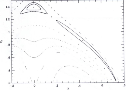
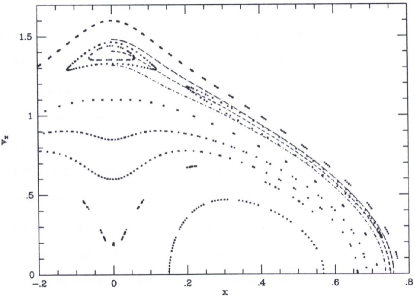
Figure 1: Using perturbation theory to model a resonant family of orbits. Dots show consequents obtained by numerical integration. The curves in the top panel show resonant orbits obtained by applying perturbation theory to orbits obtained by torus mapping. The curves in the lower panel show three of these orbits, one through the centre of the resonant region and one on each side. From Kaasalainen (1994a).

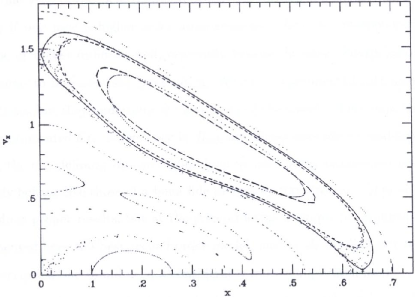
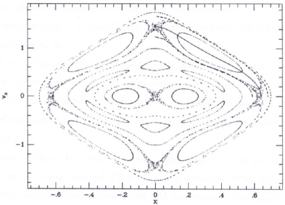
Figure 2: Obtaining resonant orbits by direct torus mapping. The lower panel shows a surface of section that is largely taken up by several powerful resonances. Three non-resonant orbits obtained by torus mapping are shown, one through the middle and one on each side of the largest resonant family. The uper panel shows several orbits of the resonant family that are obtained by directly mapping isochrone orbits. Notice that the chaotic region is nicely contained between two of these mapped orbits. From Kaasalainen (1994a).

Even in the absence of departures from axisymmetry or time-variation in the potential, resonances between the three characteristic frequencies of a quasi-periodic orbit can deform the orbital structure from that encountered in analytically integrable potentials. Important examples of this phenomenon are encountered in the dynamics of triaxial elliptical galaxies, where resonant ‘boxlets’ almost entirely replace box orbits when the potential is realistically cuspy (Merritt & Fridman 1996), and in the dynamics of disk galaxies, where the 1:1 resonance between radial and vertical oscillations probably trapped significant numbers of thick-disk stars as the mass of the thin disk built up (Sridhar & Touma 1996). Kaasalainen (1995b) has shown that such families of resonant orbits may be very successfully modelled by applying perturbation theory to orbits obtained by torus mapping. If the resonant family is exceptionally large, one may prefer to obtain its orbits directly by torus mapping (Kaasalainen 1995a) rather than through perturbation theory. Figures 1 and 2 show examples of each approach to a resonant family. Both figures show surfaces of section for motion in a planar bar. In Figure 1 a relatively weak resonance is successfuly handled through perturbation theory, while in Figure 2 a more powerful resonance that induces significant chaos is handled by directly mapping isochrone orbits into the resonant region. These examples demonstrate that if we obtain orbits by torus mapping, we will be able to discover what the Galaxy would look like in the absence of any particular resonant family or chaotic region, so we will be able to ascribe particular features in the data to particular resonances and chaotic zones. This facility will make the modelling process more instructive than it would be if we adopted a simple orbit-based technique.

5 Confronting the data

A dynamical model Galaxy will consist of a gravitational potential $\Phi({\bf x})$ together with distribution functions $f_{\alpha}({\bf J})$ for each of several stellar populations. Each distribution function may be represented by a set of orbital weights $w_{i}$, and the populations will consist of probability distributions in mass $m$, metallicity $Z$ and age $\tau$ that a star picked from the population has the specified characteristics. Thus a Galaxy model will contain an extremely large number of parameters, and fitting these to the data will be a formidable task.

Since so much of the Galaxy will be hidden from GAIA by dust, interpretation of the GAIA catalogue will require a knowledge of the three-dimensional distribution of dust. Such a model can be developed by the classical method of comparing measured colours with the intrinsic colours of stars of known spectral type and distance. At large distances from the Sun, even GAIA’s small parallax errors will give rise to significantly uncertain distances, and these uncertainties will be an important limitation on the reliability of any dust model that one builds in this way.

Dynamical modelling offers the opportunity to refine our dust model because Newton’s laws of motion enable us to predict the luminosity density in obscured regions from the densities and velocities that we see elsewhere, and hence to detect obscuration without using colour data. Moreover, they require that the luminosity distributions of hot components are intrinsically smooth, so fluctuations in the star counts of these populations at high spatial frequencies must arise from small scale structure in the obscuring dust. Therefore, we should solve for the distribution of dust at the same time as we are solving for the potential and the orbital weights.

In principle one would like to fit a Galaxy model to the data by predicting from the model the probability density $P(\alpha,\ldots,v)$ of detecting a star at given values of the catalogue variables, such as celestial coordinates $\alpha$, parallax $\varpi$, and proper motons $\mu$, and then evaluating the likelihood $L=\prod_{i}P_{i}$, where the product runs over stars in the catalogue and

$$P_{i}=\int{\rm d}^{2}\alpha\,{\rm d}\varpi\,{\rm d}^{2}\mu\,{\rm d}v\,{{\rm e}^{-(\alpha-\alpha_{i})^{2}/2\sigma^{2}_{\alpha}}\over 2\pi\sigma^{2}_{\alpha}}$$

$$\times\cdots\times{{\rm e}^{-(v-v_{i})^{2}/2\sigma^{2}_{v}}\over(2\pi\sigma^{2}_{v})^{1/2}}\,P(\alpha,\ldots,v)$$ (5)

with $\alpha_{i}\ldots v_{i}$ the measured values and $\sigma_{\alpha}\ldots\sigma_{v}$ the associated uncertainties. Unfortunately, it is likely to prove difficult to obtain the required probability density $P$ from an orbit-based model, and we will be obliged to compare the real catalogue to a pseudo-catalogue derived from the current model. Moreover, standard optimization algorithms are unlikely to find the global maximum in $L$ without significant astrophysical input from the modeller. In any event, evaluating $P_{i}$ for each of $\sim 10^{9}$ observed stars is a formidable computational problem. Devising efficient ways of fitting models to the data clearly requires much more thought.

5.1 Adaptive dynamics

Fine structure in the Galaxy’s phase space may provide crucial assistance in fitting a model to the data. Two inevitable sources of fine structure are (a) resonances, and (b) tidal streams. Resonances will sometimes be marked by a sharp increase in the density of stars, as a consequence of resonant trapping, while other resonances show a deficit of stars. Suppose the data seem to require an enhanced density of stars at some point in action space and you suspect that the enhancement is caused by a particular resonance. By virtue of errors in the adopted potential $\Phi$, the frequencies will not actually be in resonance at the centre of the enhancement. By appropriate modification of $\Phi$ it will be straightforward to bring the frequencies into resonance. By reducing the errors in the estimated actions of orbits, a successful update of $\Phi$ will probably enhance the overdensity around the resonance. In fact, one might use the visibility of density enhancements to adjust $\Phi$ very much as the visibility of stellar images is used with adaptive optics to configure the telescope optics.

A tidal stream is a population of stars that are on very similar orbits – the actions of the stars are narrowly distributed around the actions of the orbit on which the dwarf galaxy or globular cluster was captured. Consequently, in action space a tidal stream has higher contrast than it does in real space, where the stars’ diverging angle variables gradually spread the stars over the sky. Errors in $\Phi$ will tend to disperse a tidal stream in action space, so again $\Phi$ can be tuned by making the tidal stream as sharp a feature as possible.

6 Conclusions

Dynamical Galaxy models have a central role to play in attaining GAIA’s core goal of determining the structure and unravelling the history of the Milky Way. Even though people have been building Galaxy models for over half a century, we are still only beginning to construct fully dynamical models, and we are very far from being able to build multi-component dynamical models of the type that the GAIA will require.

At least three potentially viable Galaxy-modelling technologies can be identified. One has been extensively used to model external galaxies, one has the distinction of having been used to build the currently leading Galaxy model, while the third technology is the least developed but potentially the most powerful. At this point we would be wise to pursue all three technologies.

Once constructed, a model needs to be confronted with the data. On account of the important roles in this confrontation that will be played by obscuration and parallax errors, there is no doubt in my mind that we need to project the models into the space of GAIA’s catalogue variables $(\alpha,\varpi,\ldots)$. This projection is simple in principle, but will be computationally intensive in practice.

The third and final task is to change the model to make it fit the data better. This task is going to be extremely hard, and it is not clear at this point what strategy we should adopt when addressing it. It seems possible that features in the action-space density of stars associated with resonances and tidal streams will help us to home in on the correct potential.

There is much to do and it is time we started doing it if we want to have a reasonably complete box of tools in hand when the first data arrive in 2012–2013. The overall task is almost certainly too large for a single institution to complete on its own, and the final galaxy-modelling machinery ought to be at the disposal of the wider community than the dynamics community since it will be required to evaluate the observable implications of any change in the characteristics or kinematics of stars or interstellar matter throughout the Galaxy. Therefore, we should approach the problem of building Galaxy models as an aspect of infrastructure work for GAIA, rather than mere science exploitation.

I hope that in the course of the next year interested parties will enter into discussions about how we might divide up the work, and define interface standards that will enable the efforts of different groups to be combined in different combinations. It is to be hoped that these discussions lead before long to successful applications to funding bodies for the resources that will be required to put the necessary infrastructure in place by 2012.

References

- Alcock et al. (2000) Alcock, C., et al., 2000, ApJ, 541, 734
- Afonso, et al. (2003) Afonso, C., Albert J., Alard C., et al., 2003, A&A, 404, 145
- Bahcall & Soneira (1980) Bahcall, J.N. & Soneira, R.M., 1980, ApJS, 44, 73
- Bahcall & Soneira (1984) Bahcall, J.N. & Soneira, R.M., 1984, ApJS, 55, 67