astro-ph/0411209 Cosmic Acceleration and Modified Gravitational Models

Abstract

There is now overwhelming observational evidence that our Universe is accelerating in its expansion. I discuss how modified gravitational models can provide an explanation for this observed late-time cosmic acceleration. We consider specific low-curvature corrections to the Einstein-Hilbert action. Many of these models generically contain unstable de Sitter solutions and, depending on the parameters of the theory, late-time accelerating attractor solutions.

1 Introduction

One of the most profound discoveries of observational physics is that the universe is accelerating in its expansion. Evidence for this acceleration is provided by recent supernovae data together with measured CMB anisotropies and large scale structure data [1]. Despite a large number of attempts to explain this striking phenomenon (for example, dark energy associated to some new scalar field [2] or a cosmological constant [3]) all current models require at least some degree of fine-tuning and are incomplete. Due to the lack of a satisfactory explanation, it seems reasonable to consider the possibility that the observed acceleration is an indication that General Relativity requires some sort of low-energy modification [4, 5]. This radical possibility motivated the recent work of Carroll, Duvvuri, Trodden and Turner (CDTT) [5]. These authors considered a simple modification to the Einstein-Hilbert action of the form $R^{n}$, with $n<0$. They showed that under certain circumstances such models can lead to late-time acceleration of the expanding universe. In these notes, I review the basic principles of the CDTT model and explain how these principles can be applied to more general modified graviational models [6].

2 Modifications of General Relativity

The cosmic evolution of our Universe is believed to be described by the Einstein-Hilbert action (coupled to matter)

$$S=\frac{M_{\rm P}^{2}}{2}\int d^{4}\!x\,\sqrt{-g}\,R+\int d^{4}\!x\,\sqrt{-g}\,{\mathcal{L}}_{m}\,,$$ (2.1)

where $M_{\rm P}\equiv(8\pi G)^{-1/2}$ is the reduced Planck mass, $R$ is the Ricci Scalar constructed from the metric tensor $g_{\mu\nu}$ and ${\mathcal{L}}_{m}$ represents some matter Lagrangian. Let us consider modifications of (2.1), of the general form

$$S=\frac{M_{\rm P}^{2}}{2}\int d^{4}\!x\,\sqrt{-g}\,F(R,\,R_{\mu\nu}R^{\mu\nu},\,R_{\mu\nu\lambda\sigma}R^{\mu\nu\lambda\sigma},\dots)+\int d^{4}\!x\,\sqrt{-g}\,{\mathcal{L}}_{m}\,,$$ (2.2)

where $R_{\mu\nu}$ and $R_{\mu\nu\lambda\sigma}$ are the Ricci and Riemann tensors, respectively. In the literature, such modifications have been used to obtain early-time inflation (for example, Starobinsky considered $F(R)=R+R^{2}+$conformal anomaly in [7]) and to try to eliminate curvature singularities in cosmological and black hole spacetimes [8]. Unlike these high curvature examples, in order to explain late-time cosmic acceleration, we are interested in modifications that become important at low curvatures. We will see that such modified models can lead to late-time accelerating vacuum solutions, providing a purely gravitational alternative to dark energy.

2.1 The CDTT Model

The first examples of these low-curvature modifications where presented by CDTT and involved simple inverse-powers of the Ricci Scalar (i.e. $F(R)=R+mR^{n}$, where $n<0$ and $m$ is some new scale in the theory) [5]. By considering only inverse powers of $R$, we exclude Minkowski space as a solution and ensure that the correction term dominates the action only at low curvatures. As a toy model, consider the case when $n=-1$,

$$S=\frac{M_{\rm P}^{2}}{2}\int d^{4}\!x\,\sqrt{-g}\,\left(R-\frac{\mu^{4}}{R}\right)+\int d^{4}\!x\,\sqrt{-g}\,{\mathcal{L}}_{m}\,.$$ (2.3)

Here $\mu$ is a new scale in the theory with dimensions of mass. Assuming a flat, Friedmann-Robertson-Walker (FRW) metric:

$$ds^{2}=-dt^{2}+a^{2}(t)d{\b{x}}^{2}\,,$$ (2.4)

the modified Friedmann equation (in terms of the Hubble parameter $H\equiv\dot{a}/a$) is

$$3H^{2}-\frac{\mu^{4}}{12({\dot{H}}+2H^{2})^{3}}\left(2H{\ddot{H}}+15H^{2}{\dot{H}}+2{\dot{H}}^{2}+6H^{4}\right)=\frac{\rho_{m}}{M_{\rm P}^{2}}\,$$ (2.5)

where $\rho_{m}$ is the matter energy density and we have assumed a perfect-fluid energy-momentum tensor

$$T_{\mu\nu}=(\rho_{m}+P_{m})u_{\mu}u_{\nu}+P_{m}g_{\mu\nu}\,.$$ (2.6)

It is a trivial task to map this theory to an Einstein frame with Einstein-Hilbert action minimally coupled to a scalar field $\varphi$ with potential

$$V(\varphi)=\mu^{2}M_{\rm P}^{2}\exp\left(-2\sqrt{\frac{2}{3}}\frac{\varphi}{M_{\rm P}}\right)\sqrt{\exp\left(\sqrt{\frac{2}{3}}\frac{\varphi}{M_{\rm P}}\right)-1}\,.$$ (2.7)

This potential is plotted in Fig. (1).

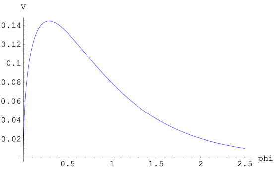
Figure 1: Plot of the potential $V(\varphi)$ in Eq. (2.7).

In this model there is a singularity corresponding to $\varphi=0$. From the plot of $V(\varphi)$ it is clear that this model exhibits three different possible cosmological behaviors, depending on the initial conditions for the field $\varphi_{i}$ and its velocity $\varphi^{\prime}_{i}$ (where the prime denotes differentiation with respect to the cosmic time coordinate of the Einstein frame). The field $\varphi$ can either roll back down the potential toward a future singularity at $\varphi=0$, come to rest at the top of the potential (corresponding to an unstable de Sitter phase) or roll off to infinity leading to late-time, power-law cosmic acceleration with equation of state parameter $w_{eff}=-2/3$. These basic features are not affected by the addition of matter. By choosing $\mu\simeq 10^{-33}eV$, the modifications to Einstein gravity only become important recently, making this theory a candidate to explain the observed acceleration of the Universe. It is important to point out this model is different from other models with scalar fields that attempt to explain dark energy, because our field is non-minimally coupled to matter. If the matter is added directly in the gravity frame (2.3), the Einstein-frame matter density is related to $\rho$ by

$$\tilde{\rho}=\exp\left(-2\sqrt{\frac{2}{3}}\frac{\varphi}{M_{\rm P}}\right)\rho\,.$$ (2.8)

This simple model is easily generalized to corrections of the form $-\mu^{2(n+1)}/R^{n}$. These generalizations maintain the desirable late-time accelerating solutions with behavior analogous to dark energy with equation of state parameter

$$w_{eff}=-1+\frac{2(n+2)}{3(2n+1)(n+1)}\,.$$ (2.9)

It is, therefore, easy to construct models of this type that obey the observational constraints on the equation of state parameter $-1.45<w<-.74$ (at the 95% confidence level) [9]. These simple models provide a new approach to understanding the dark energy problem.

2.1.1 Solar System Constraints

$F(R)$ theories can have difficulties satisfying certain observational constraints (for example, solar system constraints) [10]. A simple way to understand this is the following. By introducing a new scalar field $\phi$, the action (2.2) with $F$ a function only of $R$, is equivalent to

$$S=\frac{M_{\rm P}^{2}}{2}\int d^{4}\!x\,\sqrt{-g}\,\left(F(\phi)+F^{\prime}(\phi)(R-\phi)\right)+\int d^{4}\!x\,\sqrt{-g}\,{\mathcal{L}}_{m}\,,$$ (2.10)

where prime denotes differentiation with respect to $\phi$. The absence of a kinetic term for $\phi$ in (2.10), means that this theory can be written as a Brans-Dicke type theory, which is of the general form:

$$S\simeq\int d^{4}\!x\,\sqrt{-\bar{g}}\,\left(\Phi R-\frac{\omega}{\Phi}\partial_{\mu}\Phi\partial^{\mu}\Phi-U(\Phi)\right)+S_{m}\,,$$ (2.11)

with Brans-Dicke parameter $\omega=0$. If the scalar field is very light (as in the CDTT model) there are constraints on $\omega$ from solar system tests that give $\omega>40,000$ [11].

3 Generalized Modified Gravity Models

As we have seen, the ability to map the $F(R)$ theory to an Einstein frame makes interpretation of solutions particularly simple. In these notes we would like to consider more complicated modifications such as $F(R,\,R_{\mu\nu}R^{\mu\nu},\,R_{\mu\nu\lambda\sigma}R^{\mu\nu\lambda\sigma},\dots)$. It is not always possible to map these general models to a familiar Einstein frame and we must, therefore, develop new methods for studying such systems. A specific technique is presented in our recent paper [6].

Here we discuss a few simple examples of more general modified gravitational models. To begin we search for general features of such models. Consider the action

$$S=\int\,d^{4}\!x\,\left(R+f(R,P,Q)\right)+\int d^{4}\!x\,\sqrt{-g}\,{\mathcal{L}}_{m}\,,$$ (3.12)

with $P\equiv R_{\mu\nu}R^{\mu\nu}$ and $Q\equiv R_{\mu\nu\lambda\sigma}R^{\mu\nu\lambda\sigma}$. By defining $f_{R}\equiv\partial f/\partial R$, $f_{P}\equiv\partial f/\partial P$ and $f_{Q}\equiv\partial f/\partial Q$, the equations of motion derived from (3.12) are

$$R_{\mu\nu} - {1\over 2}\,g_{\mu\nu}\,R-{1\over 2}\,g_{\mu\nu}\,f$$ (3.13)

$$+ f_{R}\,R_{\mu\nu}+2f_{P}\,R^{\alpha}{}_{\mu}\,R_{\alpha\nu}+2f_{Q}\,R_{\alpha\beta\gamma\mu}\,R^{\alpha\beta\gamma}{}_{\nu}$$

$$+ g_{\mu\nu}\,\Box f_{R}-\nabla_{\mu}\nabla_{\nu}f_{R}-2\nabla_{\alpha}\nabla_{\beta}[f_{P}\,R^{\alpha}{}_{(\mu}{}\delta^{\beta}{}_{\nu)}]+\Box(f_{P}\,R_{\mu\nu})$$

$$+ g_{\mu\nu}\,\nabla_{\alpha}\nabla_{\beta}(f_{P}\,R^{\alpha\beta})-4\nabla_{\alpha}\nabla_{\beta}[f_{Q}\,R^{\alpha}{}_{(\mu\nu)}{}^{\beta}]=8\pi G\,T_{\mu\nu}\ .$$

Let us focus on vacuum solutions to the above field equations. This is physically well motivate since we are interested in studying the new cosmological features induced by the purely gravitational sector of the theory. Mathematically, this provides us with valuable insight into the structure of the equations.

To ensure that Minkowski space is not an allowed solution we consider modifications involving inverse powers of curvature invariants. It is likely that the addition of such terms will introduce ghost degrees of freedom into the theory. If ghosts arise we shall require that some unknown mechanism (for example, extra-dimensional effects) cut off the theory in such a way that the associated instabilities do not appear on cosmological time scales.

The first general feature of the vacuum solutions of (3.13), is the existence of constant curvature solutions. To see this, we take the trace of (3.13) and substitute $Q=R^{2}/4$ and $P=R^{2}/6$ (which are identities satisfied by constant curvature spacetimes) into the resulting equation to obtain the algebraic equation:

$$\left(2f_{Q}+3f_{P}\right)R^{2}+6\left(f_{R}-1\right)R-12f=0\ .$$ (3.14)

Solving this equation for the Ricci scalar yields the constant curvature (de Sitter) vacuum solutions with $R\neq 0$. This is a very general property of actions of the form (3.12). However, an equally generic feature of such models is that this de Sitter solution is unstable. In the CDTT model, the instability is to an accelerating power-law attractor. We will see a similar trend in many of the more general models under consideration here.

For simplicity, we now specialize to a class of actions with

$$f(R,P,Q)=-\frac{\mu^{4n+2}}{(aR^{2}+bP+cQ)^{n}}\ ,$$ (3.15)

where $n$ is a positive integer, $\mu$ has dimensions of mass and $a$, $b$ and $c$ are dimensionless constants. In this case, there are power-law attractors with the following (real) exponents

$$v^{\rm gen}_{1,2}=\frac{8n^{2}+10n+2-3\alpha\pm\sqrt{\Gamma}}{4(n+1)}\ ,$$ (3.16)

where

$$\Gamma=9n^{2}\alpha^{2}-(80n^{3}+116n^{2}+40n+4)\,\alpha+64n^{4}+160n^{3}+132n^{2}+40n+4\ .$$ (3.17)

Two special cases are

$$f = -\frac{m^{4n+2}}{P^{n}}\ ,$$

$$f = -\frac{M^{4n+2}}{Q^{n}}\ ,$$ (3.18)

for which the power law attractors, $v_{1,2}$ are

$$v^{(P)}_{1,2} = \frac{12n^{2}+9n+3\pm\sqrt{144n^{2}+120n^{3}-15n^{2}-30n-3}}{2(3+3n)}$$ (3.19)

$$v^{(Q)}_{1,2} = \frac{4n^{2}+2n+1\pm\sqrt{16n^{4}-16n^{2}-10n-1}}{2n+2}\ .$$ (3.20)

Having discovered some basic common features of these general models (de Sitter repeller and power-law attractor solutions), let us consider some specific examples in greater detail.

3.1 Inverse powers of R

For the simplest case, when $f(R)=-\mu^{4}/R$, the model is simply that of CDTT with modified Friedmann equation given by (2.5). One way to analyze this system (without going to an Einstein frame) is to simply plot the phase space of solutions (see Fig.(2)).

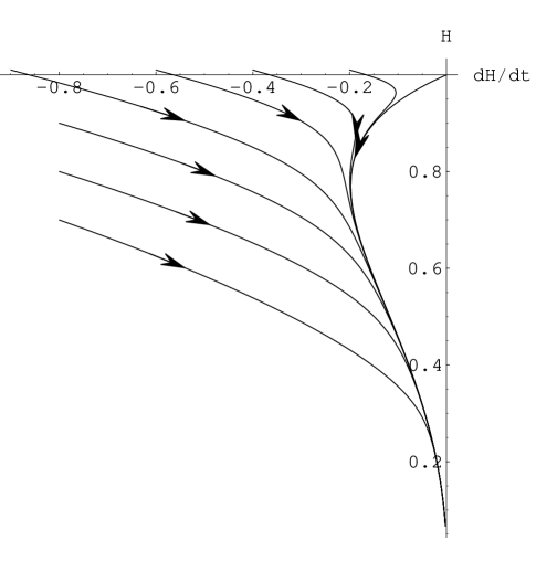
Figure 2: Phase portrait for the CDTT model with $f(R)=1/R$. The unstable de Sitter solution is at the point $(0,1)$. Solutions that are initially not accelerating ($\ddot{a}<0$) evolve toward the power-law, accelerating attractor (with $\ddot{a}>0$).

Recall, a generic feature of the models considered here is an unstable de Sitter solution (obtained from Eq. (3.14)). For the above case of $f(R)=1/R$, the de Sitter solution is located at the point $(0,1)$ in the $(\dot{H},H)$-phase plane depicted in Fig.(2). The late time power law attractor has $a(t)\propto t^{p}$, $H=p/t$ and $\dot{H}=-p/t^{2}$. Hence, such attractor solutions appear as curves $H=\sqrt{-p\dot{H}}$, ($\dot{H}<0$) in the phase portrait. In the case $1/R$, there is only one late-time power-law attractor with $p=2$. Following this example, we proceed to examine more complicated modified theories.

3.2 Inverse powers of $P\equiv R_{\mu\nu}R^{\mu\nu}$

Consider a modification of the form $f(P)=-\mu^{6}/P$. The trace equation (3.14), indicates the de Sitter constant curvature solution occurs for $R^{(P)}_{dS}=(16)^{1/3}\mu^{2}$.

The modified Friedmann equation takes the form

$$\frac{1}{8(3H^{4}+3H^{2}\dot{H}+\dot{H}^{2})^{3}} = (24H^{2}\dot{H}^{6}+216H^{4}\dot{H}^{5}+\mu^{6}\dot{H}^{4}+864H^{6}\dot{H}^{4}$$ (3.21)

$$+ 11\mu^{6}H^{2}\dot{H}^{3}+1944H^{8}\dot{H}^{3}+2\mu^{6}H\dot{H}^{2}\ddot{H}$$

$$+ 33\mu^{6}H^{4}\dot{H}^{2}+2592H^{10}\dot{H}^{2}+30\mu^{6}H^{6}\dot{H}$$

$$+ 6\mu^{6}H^{3}\dot{H}\ddot{H}+1944H^{12}\dot{H}+6\mu^{6}H^{8}$$

$$+ 648H^{14}+4\mu^{6}H^{5}\ddot{H})=0\,.$$

and power-law attractors are identified by substituting a power-law ansatz $H(t)=p/t$ and taking the late-time limit. By defining $v=-\dot{H}/H$ and requiring $v$ to be a constant $v_{0}=p$ we find the condition

$$6v_{0}^{4}-30v_{0}^{3}+41v_{0}^{2}-23v_{0}+5=0\ .$$ (3.22)

which gives two late-time power-law attractors with $p=2\pm\sqrt{6}/2$. One of these corresponds to an accelerator with $p\simeq 3.22$, while the other is not an accelerating solution with $p\simeq.77$. Both attractor solutions along with the de Sitter solution are easily identified in the phase space portrait given in Fig. (3).

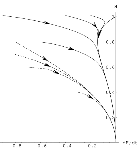
Figure 3: Phase portrait for $f(R)=1/R_{\mu\nu}R^{\mu\nu}$. The unstable de Sitter solution is at the point $(0,1)$. The two late-time power-law attractors are clearly visible for $p\simeq.77$ (dashed lines) and $p\simeq 3.22$ (solid lines).

3.3 Inverse powers of $Q\equiv R_{\mu\nu\lambda\sigma}R^{\mu\nu\lambda\sigma}$

In the case of $f(Q)=-\mu^{6}/Q$ we find from the trace equation that the constant curvature de Sitter solution is given by $R^{(Q)}_{dS}=(24)^{1/3}\mu^{2}$. The modified Friedmann equation is

$$\frac{1}{24[\dot{H}^{2}+2H^{2}\dot{H}+2H^{4}]^{3}}\left[576H^{14}+1728H^{12}\dot{H}+2592H^{10}\dot{H}^{2}+2304H^{8}\dot{H}^{3}\right.$$

$$+1296H^{6}\dot{H}^{4}+432H^{4}\dot{H}^{5}+72H^{2}\dot{H}^{6}+8\mu^{6}H^{8}+36\mu^{6}H^{6}\dot{H}+54\mu^{6}H^{4}\dot{H}^{2}$$

$$+20\mu^{6}H^{2}\dot{H}^{3}\left.+3\mu^{6}\dot{H}^{4}+4\mu^{6}H^{5}\ddot{H}+12\mu^{6}H^{3}\dot{H}\ddot{H}+6\mu^{6}H\dot{H}^{2}\ddot{H}\right]=0\ ,$$ (3.23)

which does not admit any late-time power-law attractors.

4 Conclusions

We have described how a late-time period of cosmic acceleration emerges naturally in certain modified gravitational models. The models in [6] involve inverse powers of linear combinations of curvature invariants. Clearly, the modified gravitational models described in these notes are only a small handful of a much richer set of possible theories. The late-time accelerating vacuum solutions we have discussed are not severely affected by the inclusion of matter. A simple way to understand this is the following. In an expanding universe the curvature invariants $R^{n}$, $P$ and $Q$ are all decreasing with time. Therefore, any modifications of Einstein gravity that are inverse powers of such invariants are growing with time. If the universe is initially matter dominated, these growing correction terms will eventually come to dominate the action. 

It is an intriguing possibility that the observed cosmic acceleration of our universe may be a consequence of some low-curvature modified gravitational theory. A first attempt to explore this possibility was made in [6]. It is important that we try to better understand these models and the observational constaints on low energy modifications of GR.

References

- [1] A. G. Riess et al. Astron. J. 116, 1009 (1998); S. Perlmutter et al. Astrophys. J. 517, 565 (1999); J. L. Tonry et al., Astrophys. J. 594, 1 (2003); C. L. Bennett et al., Astrophys. J. Suppl. 148, 1 (2003); C. B. Netterfield et al. Astrophys. J. 571, 604 (2002); N. W. Halverson et al., Astrophys. J. 568, 38 (2002).
- [2] C. Wetterich, Nucl. Phys. B 302, 668 (1988); B. Ratra and P. J. E. Peebles, Phys. Rev. D 37, 3406 (1988); R. R. Caldwell, R. Dave and P. J. Steinhardt, Phys. Rev. Lett. 80, 1582 (1998); C. Armendariz-Picon, T. Damour and V. Mukhanov, Phys. Lett. B 458, 209 (1999); C. Armendariz-Picon, V. Mukhanov and P. J. Steinhardt, Phys. Rev. Lett. 85, 4438 (2000); C. Armendariz-Picon, V. Mukhanov and P. J. Steinhardt, Phys. Rev. D 63, 103510 (2001); L. Mersini, M. Bastero-Gil and P. Kanti, Phys. Rev. D 64, 043508 (2001); R. R. Caldwell, Phys. Lett. B 545, 23 (2002); S. M. Carroll, M. Hoffman and M. Trodden, Phys. Rev. D 68, 023509 (2003); V. Sahni and A. A. Starobinsky, Int. J. Mod. Phys. D 9, 373 (2000); L. Parker and A. Raval, Phys. Rev. D 60, 063512 (1999) [Erratum-ibid. D 67, 029901 (2003)].
- [3] For reviews see, e.g., S. M. Carroll, Living Rev. Rel. 4, 1 (2001); P. J. E. Peebles and B. Ratra, Rev. Mod. Phys. 75, 559 (2003); T. Padmanabhan, Phys. Rept. 380, 235 (2003).
- [4] C. Deffayet, G. R. Dvali and G. Gabadadze, Phys. Rev. D 65, 044023 (2002); K. Freese and M. Lewis, Phys. Lett. B 540, 1 (2002); M. Ahmed, S. Dodelson, P. B. Greene and R. Sorkin, Phys. Rev. D 69, 103523 (2004); N. Arkani-Hamed, S. Dimopoulos, G. Dvali and G. Gabadadze, arXiv:hep-th/0209227; G. Dvali and M. S. Turner, arXiv:astro-ph/0301510; G. Dvali, arXiv:hep-th/0402130; A. Padilla, arXiv:hep-th/0406157; G. Allemandi, A. Borowiec and M. Francaviglia, arXiv:hep-th/0407090; A. Padilla, arXiv:hep-th/0410033.
- [5] S. M. Carroll, V. Duvvuri, M. Trodden and M. S. Turner, Phys. Rev. D 70, 043528 (2004) [arXiv:astro-ph/0306438].
-
[6]
S. M. Carroll, A. De Felice, V. Duvvuri, D. A. Easson, M. Trodden and M. S. Turner,
arXiv:astro-ph/0410031. - [7] A. A. Starobinsky, Phys. Lett. B 91, 99 (1980).
- [8] V. P. Frolov, M. A. Markov and V. F. Mukhanov, Phys. Lett. B 216, 272 (1989). V. P. Frolov, M. A. Markov and V. F. Mukhanov, Phys. Rev. D 41, 383 (1990). V. Mukhanov and R. H. Brandenberger, Phys. Rev. Lett. 68, 1969 (1992); M. Trodden, V. F. Mukhanov and R. H. Brandenberger, Phys. Lett. B 316, 483 (1993); R. H. Brandenberger, V. Mukhanov and A. Sornborger, Phys. Rev. D 48, 1629 (1993); R. Moessner and M. Trodden, Phys. Rev. D 51, 2801 (1995); R. H. Brandenberger, R. Easther and J. Maia, JHEP 9808, 007 (1998); D. A. Easson and R. H. Brandenberger, JHEP 9909, 003 (1999); D. A. Easson and R. H. Brandenberger, JHEP 0106, 024 (2001); D. A. Easson, JHEP 0302, 037 (2003); D. A. Easson, Phys. Rev. D 68, 043514 (2003).
- [9] A. Melchiorri, L. Mersini, C. J. Odman and M. Trodden, Phys. Rev. D 68, 043509 (2003) [arXiv:astro-ph/0211522]; D. N. Spergel et al., Astrophys. J. Suppl. 148, 175 (2003).
- [10] T. Chiba, arXiv:astro-ph/0307338; E. E. Flanagan, Phys. Rev. Lett. 92, 071101 (2004); M. E. Soussa and R. P. Woodard, Gen. Rel. Grav. 36, 855 (2004); G. Dvali, arXiv:hep-th/0402130; A. Nunez and S. Solganik, arXiv:hep-th/0403159.
- [11] B. Bertotti, L. Iess and P. Tortora, Nature 425, 374 (2003).
- [12] S. Nojiri and S. D. Odintsov, Phys. Rev. D 68, 123512 (2003); S. Nojiri and S. D. Odintsov, Gen. Rel. Grav. 36, 1765 (2004); S. Nojiri and S. D. Odintsov, Mod. Phys. Lett. A 19, 627 (2004).