Interpretations of gamma-ray burst spectroscopy
I. Analytical and numerical study of spectral lags

We describe the strong spectral evolution that occurs during a gamma-ray burst (GRB) pulse and the means by which it can be analyzed. In particular, we discuss the change of the light curve as a function of energy and the spectral lag. Based on observed empirical correlations, an analytical model is constructed which is used to describe the pulse shape and quantize the spectral lags and their dependences on the spectral evolution parameters. Using this model, we find that the spectral lag depends mainly on the pulse-decay time-scale and that hard spectra (with large spectral power-law indices $\alpha$) give the largest lags. Similarly, large initial peak-energies, $E_{\rm 0}$, lead to large lags, except in the case of very soft spectra. The hardness ratio is found to depend only weakly on $\alpha$ and the hardness-intensity–correlation index, $\eta$. In particular, for low $E_{\rm 0}$, it is practically independent, and is determined mainly by $E_{\rm 0}$. The relation between the hardness ratio and the lags, for a certain $E_{\rm 0}$ are described by power-laws, as $\alpha$ varies. These results are the consequences of the empirical description of the spectral evolution in pulses and can be used as a reference in analyses of observed pulses. We also discuss the expected signatures of a sample of hard spectral pulses (e.g. thermal or small pitch-angle synchrotron emission) versus soft spectral pulses (e.g. optically-thin synchrotron emission). Also the expected differences between a sample of low energetic bursts (such as X-ray flashes) and of high energetic bursts (classical bursts) are discussed.

1 Introduction

The analysis of the prompt emission from gamma-ray bursts (GRBs) is giving us valuable clues to the environment from which the radiation emanates. Much evidence points to the fact that the gamma radiation stems from dissipation processes in a relativistically expanding plasma wind (Rees & Mészáros, 1992; Mészáros, 2002), either as shocks or in magnetic reconnections. Complex and variable light curves, that consist of several, often overlapping spikes or pulses, tell us through their variability and spectral power distribution about the energetics (Kumar, 1999), radial structure of the fireball (Beloborodov, 2000), and can even give hints about the progenitor (Kobayashi et al. (2002); Salmonson & Galama (2002)). Individual pulses, which are assumed to be related to single emission episodes, give us information on the microphysics; radiation processes (Piran, 1999), and comoving properties of the fireball, such as the densities and magnetic fields (Ryde & Petrosian, 2002). We will here review the various spectroscopic analysis methods that are used to characterize the spectral evolution during bursts and especially during their constituent pulses. We will examine the analysis of the spectral lags between the light curves, measured in different energy bands, and how these results compare to the high-resolution spectroscopic analysis in which the time-evolution and correlations of spectral parameters are deduced. The latter approach is useful as it can be used directly to test models of the dynamics and the emission processes. However, it can only be performed on cases in which we have high-resolution spectra and know their time-evolution. On the other hand, the lag description has the advantage that it can be measured on practically every GRB, even weak ones, from all satellite missions which have more than one spectral channel. Moreover, several relations have been identified between the spectral lag and the physical quantities of the burst, such as the isotropically equivalent luminosity (Norris, Marani, & Bonnell (2000)) and the peak energy of the spectrum (Amati et al. (2002)). It is therefore of interest to understand how these two descriptions relate to each other, since this will facilitate the interpretation of the spectral lag, and its dependence on other parameters.

The observation that the light-curves in different energy bands lag behind each other is a common feature in astrophysical objects, and is not only found in GRBs. There are several physical scenarios in which this can be explained. Positive lags, that is, the soft radiation lagging the hard, which is the dominant behavior observed in GRBs, can be due to an intrinsic cooling of the radiating electrons, which will cause the radiation to dominate at lower and lower energies. Alternatively, a Compton reflection of a medium at a sufficient distance from the initial hard source will also cause a lag. Also, a convex surface that emits at relativistic speeds will cause the radiation emitted off axis, to be delayed and softened, thus producing a lag, that is, the curvature effect (Ryde & Petrosian (2002)). Furthermore, if there were an intrinsic time-scale that is constant from burst to burst, the change in viewing angle between the object and the observer, will cause both the observed time-scale and intensity to vary in a specific way due to the angular dependence of the Doppler boost (Salmonson, 2000; Ioka & Nakamura, 2001). A possible scenario for negative lags, that is, the hard radiation lagging behind the soft, is a hot medium, say a lepton cloud surrounding a cooler emitter, which will cause the soft radiation to be upscattered by inverse Comptonization. The photons get harder the more scatterings they suffer and thus they are more delayed. A definite answer to the reason for the spectral lags in GRBs has not yet been given.

We will expand the spectral-lag analysis done sofar (denoted here as low-resolution spectroscopy, LRS: see, e.g., Band (1997) and references therein) by connecting it to the detailed spectral-evolution description that can be done for strong pulses (denoted here as high-resolution spectroscopy, HRS: see, e.g., Ford et al. (1995); Crider et al. (1997); Ryde & Svensson (2002)). The HRS and LRS are reviewed in Sect. 2 and in Sect. 3 we give an analytical treatment assuming a simple pulse model. The general empirical behavior of bursts, found through the observations made by the Burst and Transient Source Experiment (BATSE) on the Compton Gamma-Ray Observatory and their parameter distributions, are used in combination with the analytical findings to make a numerical study in Sect. 4. We simulate realistic pulses and determine how various spectral evolutions are manifested as spectral lags. Finally, we discuss the interpretations that can be made in Sect. 5.

In a subsequent paper II (Ryde et al. 2004), we will demonstrate the results on a sample of GRB pulses observed by BATSE and discuss the spectral lag correlations and various model scenarios.

2 GRB Spectral Evolution: Empirical View

2.1 High Resolution Spectroscopy (HRS)

For the strongest BATSE pulses, spectroscopy is possible with high resolution, allowing us to deconvolve the observed count spectra through the detector response, thus providing the incoming photon spectrum. The deconvolution is done through a forward-fitting method. This is done for several time intervals during the pulse, which allows details of the energy-flux spectrum to be followed in time and thus characterize the spectral evolution. Such studies have been made for instance by Preece et al. (2000) and Ryde & Svensson (2002). However by necessity, the time-resolution becomes low and only the strongest and longest pulses can be studied in this way due to the need for high signal-to-noise ratio, SNR (Preece et al. (1998)). Using this method, the spectral evolution has been quantified in correlations between the observable parameters. The complete spectral and temporal evolution of a pulse can be characterized by three main observables, the peak of the $EF_{\rm E}$ spectrum, $E_{\rm p}(t)$, the instantaneous energy flux, $F(t)$, and the derived quantity, the energy fluence ${\cal E}(t)=\int^{t}Fdt^{\prime}$. The relations between these three observables are given by two empirical correlations:

(i) the hardness-intensity correlation (HIC; see Borgonovo & Ryde (2001)), which relates the flux of the source to the ’hardness’ of the spectrum (here represented by $E=E_{\rm p}$). For the decay phase of a pulse the most common behavior of the HIC is

$$F=F_{\rm 0}(E_{\rm p}/E_{\rm 0})^{\eta},$$ (1)

where $E_{\rm 0}$ and $F_{\rm 0}$ are the initial values of the peak energy and the energy flux at the beginning of the decay phase in each pulse and $\eta$ is the power law index. Borgonovo & Ryde (2001) studied a sample of 82 GRB pulse decays and found them to be consistent with a power law HIC in at least 57% of the cases and the power law index, $\eta$ was found to have a broad distribution peaking approximately at 2.0 : $\eta=2.0\pm 0.7$. It should be noted here that even though the fits in some cases are not necessarily statistically consistent with a power law, in principle all cases do have a hard-to-soft trend that can be approximated by a power law. Indeed, by simply lowering the required level of significance of the power-law fit, Borgonovo & Ryde (2001) showed that even 75 % of the pulses were consistent with a power law. Ryde & Svensson (2002) did derive alternative analytical descriptions of the HIC for pulses that do not follow exactly a power-law. Referring to their Fig. 1, it is however obvious that the power-law description can indeed be used as an approximate description. Below, we will therefore use the analytical expression, given by Eq. 1, to describe the general behavior of all pulses. This description will then be exact for 60-70 % of pulses.

(ii) the hardness-fluence correlation, $E_{\rm pk}({\cal E})$ (HFC; Liang & Kargatis (1996)) which relates the hardness to the time running integral of the flux, that is, the fluence. Equivalently, the HFC represents the observation that the rate of change in the hardness is proportional to the luminosity of the radiating medium (or, equivalently, to the energy density);

$$\dot{E_{\rm p}}=-\frac{F}{\Phi_{0}}.$$ (2)

This corresponds to a linear relation between the $E_{\rm p}$ and the time integrated energy flux, the energy fluence,

$$E_{\rm p}(t)=E_{\rm 0}-\frac{{\cal E}(t)}{\Phi_{\rm 0}}$$ (3)

where $\Phi_{\rm 0}$ is the decay constant. This behavior is most often seen over the entire pulse and occurs in a vast majority of pulses (Liang & Kargatis, 1996; Ryde & Svensson, 2002).

Ryde & Svensson (2000) showed that these two correlations (Eqs. [1, 3]) form a complete description of the spectral evolution and define the light curve as well. In the original description they showed that the observed photon flux, $F(E)/E$ or $F(\nu)/\nu$, can often be described by a reciprocal function in time. In Sect. 3 below we will reformulate their results in terms of the energy flux.

2.2 Low Resolution Spectroscopy (LRS)

To utilize the full temporal resolution of, for instance, the BATSE data, the deconvolution is not made and the incoming light-curves are approximated by the count light-curves. This is also the case for weaker pulses for which the analysis described in the previous section is not possible. The spectral evolution is then instead quantified through the change in shape of the pulse, in two or more broad energy bands. For instance, the four channels of the BATSE discriminator rates (64 ms time resolution) can be used, and Beppo-SAX, Hete-II/FREGATE, and Swift have similar capabilities. Evolution of the spectrum, such as variations in $E_{\rm p}$ and of the power-law slopes, will cause the light curves in the different energy-channels to be different.

To quantify this change one can measure the shift in time between light curve pulses (spectral lags) and their change in width. These can be measured directly by using an analytical prescription of the pulses, but more often they are measured with the use of correlation functions (e.g., Fenimore et al. (1995)). The spectral lag, $\Delta t$, is defined as the lag, $s$, at which the cross correlation function (CFF) between the light curves in two different spectral channels, $g$ and $h$, has its maximum:

$$\rm{CCF}(g,h)(s)=\int_{-\infty}^{\infty}g(\tau+s)h(\tau)\,d\tau.$$ (4)

If the two light curves are very similar to each other, then the maximum occurs at a lag that measures the time that one is shifted compared to the other. For a detailed discussion on the general characteristics of CCF, we refer to Band (1997) who gives the analytical expression of the CCF for a pure exponential decay (see his Fig. 1). Another way of quantifying the averaged, spectral evolution of a burst, using the LRS data, is to measure the hardness-ratio (HR) of the fluences (the time-integrated fluxes) in two channels. The HR and the CCF are not independent and their relation is often sought.

Norris, Marani, & Bonnell (2000) (see also Norris (2002)) demonstrated that there is a trend that the HR is anti-correlated with spectral lag. A similar trend also exists for the peak flux, in that the long-lag bursts all have low peak fluxes. Furthermore, the distribution of lags is dominated by short lags, as also found by Band (1997). A first step to understanding the connection between the detailed, spectral evolution and the spectral lags was taken by Kocevski & Liang (2003b). They found that the HFC parameter $\Phi_{\rm 0}$ has a nearly linear correlation with lag. An even tighter correlation was found when $\Phi_{\rm 0}$ was normalized to the peak flux. Finally, the HR and the $E_{\rm p}$ are naturally correlated. Indeed, Band et al. (2004) argued for an empirical relation where $E_{\rm p}$ is proportional to the square of the HR.

Wu & Fenimore (2000) pointed out that it is not always reliable to determine lags with CCF. This is especially the case for multi-peaked bursts, for which both the HR and the CCF give an average quantitative description. Variations of a burst’s spectrum occur both within a pulse as well as between pulses. This was conclusively shown by Band (1997), who used correlation functions and was able to conclude that $\sim 90\%$ of pulses have a hard-to-soft trend, while $\sim 80\%$ of the multi-peaked bursts have a softening trend between peaks. Varying $E_{\rm 0}$, $\eta$, and $\alpha$ between individual pulses will be important in determining the integrated spectrum, which is the spectrum that is quantified by the lags and the HRs. Wu & Fenimore (2000) also noted that the methods used to calculate the CCFs can affect the results considerably. For instance, the inclusion of time intervals when the signal is at background will clearly affect the measurements. This adds complications for the interpretation of these quantities. Below, we concentrate our study to an analytical model describing a single emission episode, resulting in an individual pulse. A comparison of the CCF measurements and the actual lags is further investigated in paper II.

3 Analytical Model

To catch the essence of the spectral evolution, we use the following simplified model: the emission episode consists of a single pulse which is assumed to be dominated by the decay phase, called a FRED pulse (fast-rise-exponential-decay). We also assume that the pulse has a monotonic decay of the spectral hardness, as measured by $E_{\rm p}$, that is, it is a hard-to-soft pulse (Ford et al. (1995)). The motivation to study such a model is, first, that it is the individual pulses that bear the important physical signatures of the emission processes and these signatures are revealed mainly in the decay phase (Ryde & Petrosian (2002)). Most observed pulses do indeed have such a shape, as noted by Kocevski et al. (2003) and Ryde et al. (2003). Second, most detailed spectral evolution studies have been made on the decay phase, since it often constitutes a major part of the pulse. Third, apart from the fact that many pulses are observed to be hard-to-soft pulses, pulses for which $E_{\rm p}$ is observed to track the flux could very well still be intrinsically hard-to-soft. A motivation for this was given by Kocevski et al. (2003); pulses that are emitted prior to the analyzed one often overlap it to some extent. Since, in general, the spectra of pulses soften with time, this contamination will contribute mainly soft photons. This will cause the measured spectrum to have an $E_{\rm p}$ that is lower than that of the spectrum of the analyzed pulse itself. Below, we derive the behavior of the decay phase of a pulse and make a few analytical estimates of the dependence of the lag on various variables.

3.1 Decay Phase of a Pulse

An analytical expression for the shape of a pulse can be derived based on the knowledge of the spectral evolution. We follow the calculations first outlined in Ryde & Svensson (2000) (see also Kocevski et al. (2003)) to derive the energy-flux decay of a pulse. The combination of the two empirical relations in Eqs. (1) and (3) gives the following differential equation governing the spectral evolution

$$\dot{E_{\rm p}}=-\frac{F_{0}}{\phi_{0}E_{0}^{\eta}}E_{\rm p}^{\eta},$$ (5)

where $\dot{E_{\rm p}}$ is the time derivative of the peak energy, $F_{\rm 0}$ and $E_{\rm 0}$ are the values of the flux and the peak energy at the start of the decay phase. The solution gives the energy flux

$$F(t)=F_{\rm 0}\left(1+\frac{(\eta-1)t}{T}\right)^{-\eta/(\eta-1)}$$ (6)

and the corresponding peak energy

$$E_{\rm p}(t)=E_{\rm 0}\left(1+\frac{(\eta-1)t}{T}\right)^{-1/(\eta-1)}$$ (7)

where we have defined

$$T\equiv\Phi_{\rm 0}E_{\rm 0}/F_{\rm 0}.$$ (8)

To analyze the behavior of this function in the case $\eta=1$, we note that the denominators above both have the appearance of

$$\left(1-\frac{t/T}{n}\right)^{n},{\rm{with}}\;\;n\equiv 1/(1-\eta),$$ (9)

This expression has a limiting value of $\rm{exp}(-t/T)$ as $n\equiv(\eta-1)^{-1}\rightarrow\infty$. Therefore as $\eta$ tends to $1$, Eqs. (6) and (7) become

$$F(t)=F_{\rm 0}e^{-t/T}$$ (10)

$$E_{\rm p}(t)=E_{\rm 0}e^{-t/T}.$$ (11)

This shows that the full behavior is described by Eqs. (6) and (7) for all $\eta$. We also note that it is possible to measure $\Phi_{\rm 0}$ directly from the light curve by identifying the time scale $T=\Phi_{\rm 0}E_{\rm 0}/F_{\rm 0}$, instead of by the analysis of the spectra otherwise necessary.

Introducing $d\equiv\eta/(\eta-1)$ ($d$ as in the asymptotic decay of the energy flux) we describe the peak and the energy flux decays as

$$F(t)=F_{\rm 0}\left(1+\frac{t}{T(d-1)}\right)^{-d}$$ (12)

$$E_{\rm p}(t)=E_{\rm 0}\left(1+\frac{t}{T(d-1)}\right)^{1-d}.$$ (13)

In Sect. 4.1 we discuss an expansion of these calculations to also include the rise phase, since we will need the full description in the numerical study.

3.2 Spectral Lags

Assume now that the two spectral channels between which the lag is measured, are characterized by the energies $E_{1}$ and $E_{2}$. Assume further that the dynamical range of the change in $E_{\rm p}$ is larger or of the same order as $E_{1}/E_{2}$. These assumptions are reasonable, which can be noted in Ryde & Svensson (2002), who studied the decay of many pulse decays and found that the typical dynamic range was $\sim 4-5$ (see their Fig. 1). Including a monotonic energy decay during the rise phase of a pulse, this range will increase. Furthermore, typical values for BATSE are $E_{1}=25$ keV and $E_{2}=100$ keV. With these assumptions a portion of the non-power-law, curved photon spectrum will pass through both channels. The pulse shapes (peak and width), detected in the two channels, are then determined by how the spectral distribution changes with time; the main change of the spectrum is in the decay of $E_{\rm p}$. The spectrum will then pass through a certain channel at a speed $dE_{\rm p}/dt$ which usually changes with energy. The spectral lag can be thought of as the time it takes for the spectrum to move from $E_{1}$ to $E_{2}$, which clearly is determined by $dE_{\rm p}/dt$. Note that the actual peak, $E_{\rm p}$, does not necessarily need to pass through the channels.

Before discussing the analytical consequences of this, we will study three conceptually simple situations, which are valuable in illustrating the discussion. First, consider a situation where there is no spectral evolution, that is, the spectrum remains the same during the change in intensity; $F\propto E_{\rm p}^{\eta}$ with $\eta=\infty$. Then there will be no difference in the light curve between the bands, apart from a normalization, and the spectral lag would be zero. Second, consider a situation where we allow for a spectral evolution, but approximate the spectra with a Dirac $\delta$-function in energy (see, e.g., Cen (1999) and Ryde & Svensson (1999)) so that $F_{\rm E}(E,t)=F(t)\cdot\delta[E-E_{\rm p}(t)]$, that is, with a monochromatic spectrum. In this situation, it is clear that the time interval between the pulse peaks in the two channels is exactly the time that the spectrum takes to move from $E_{1}$ to $E_{2}$. A third situation, that is still more realistic, is to take an energy spectrum that is described by a Heavyside function, $F_{\rm E}(E,t)=F(t)\cdot\Theta[E-E_{\rm p}(t)]$, that is, the spectrum consists of two power laws with photon indices $\alpha=-1$ and $\beta=-\infty$ that are sharply joined at $E_{\rm p}$. As the break of the spectrum passes a certain energy, the flux disappears, which can constitute a characteristic point in the light curve. The difference in channel light-curves again will clearly reflect the $E_{\rm p}$ evolution.

Based on these discussions, we therefore make the following simplified model that captures the general behavior, namely that the lag, $\Delta t$, is determined by

$$\Delta t=\int_{\Delta E}\frac{dt}{dE_{\rm p}}\,dE$$ (14)

and the rate, $dE_{\rm p}/dt$, is determined by the spectral evolution parameters according to Eq.(7). Note also that, according to Eq. (2) this rate is proportional to $F/\Phi_{\rm 0}$ (see also Kocevski & Liang (2003b)). To describe this analytically, we assume that the above analytical description of the evolution of $E_{\rm p}$ is also valid for the rise phase of the pulse. Eq. (7) then gives

$$\frac{t}{T}=\frac{1}{\eta-1}\left(\left[\frac{E_{\rm 0}}{E}\right]^{\eta-1}-1\right),$$ (15)

Here, $E_{\rm 0}$ represents the maximal value of $E_{\rm p}$, that is, the value at the start of the rise phase in contrast to the definition in Sect. 3.1. This equation is also valid for all $\eta$, since as $\eta$ tends to $1$, Eq. (15) has a limiting value of

$$\frac{t}{T}=\ln\frac{E_{\rm 0}}{E}.$$ (16)

If the spectral evolution of a pulse is governed by this law, then the spectral lag, $\Delta t$, between two energy channels with characteristic energies $E_{1}$ and $E_{2}$, will be given by

$$\frac{\Delta t}{T}=\left(\frac{E_{\rm 0}}{E_{2}}\right)^{\eta-1}\frac{1}{\eta-1}\left(\left[\frac{E_{2}}{E_{1}}\right]^{\eta-1}-1\right).$$ (17)

Here $E_{1}<E_{2}$ and a positive lag is defined as the hard radiation precedes the soft. The ratio ($E_{2}/E_{1}$) in this equation is an instrumental constant and we denote the last two factors in Eq. (17) by $\psi(\eta-1)$, which tends to $\psi(0)=\ln(E_{2}/E_{1})$ as $\eta$ tends to 1. For a specific instrument the lag can thus be written as

$${\Delta t}=T\cdot(E_{\rm 0}/E_{2})^{\eta-1}\cdot\psi(\eta-1).$$ (18)

Apart from the linear dependence on $T$, the lag depends on the value of $E_{\rm 0}$ relative to the high energy channel, as well as to the instrumental function $\psi(\eta-1)$. In Eq. (18) one could have chosen to include the second factor into the instrumental function. However, the energy band of a certain instrument limits the observed values of $E_{0}$, which therefore will be correlated with the typical energy of the band. Therefore, it is useful to keep this factor separate in such a comparison. Finally, using the definition of $T$, in Eq. (8), we find that

$$\Delta t=\Phi_{\rm 0}\frac{E_{\rm 0}^{\eta}}{F_{0}}\cdot\frac{\psi(\eta-1)}{E_{2}^{\eta-1}},$$ (19)

which, as $\eta$ tends to 1, has a limiting value

$${\Delta t}=\Phi_{\rm 0}\frac{E_{\rm 0}}{F_{0}}\cdot\psi\left(0\right).$$ (20)

Figure 1: Instrumental-dependent factor, $\Psi$, as a function of the HIC index $\eta$, according to Eq. [18]. The solid line is for BATSE, the dotted line is for FREGATE, the dashed line is for Swift, and the dot-dashed line is for Beppo-SAX

In Fig. 1, the function $\psi$ is plotted versus the HIC power-law index $\eta$, for four different detectors, BATSE, Beppo-SAX, FREGATE and Swift. For BATSE, $\psi$ varies only weakly while for the other three instruments it varies somewhat more. For instance, as $\eta$ changes from 1.5 to 2.5, $\psi$ varies by a factor of 3.2 (BATSE), 5.3 (FREGATE), 7.1 (Swift), and 19 (Beppo-SAX), respectively. The typical energies used were $E_{1}/E_{2}$ = 32.5/200 (BATSE), 18.5/215 (FREGATE), 5.1/82.5 (Swift), and 7.5/370 (Beppo-SAX). The variation of $\psi$ for BATSE is relatively small, while spectral lags vary over several orders of magnitude (Norris, Marani, & Bonnell, 2000). Furthermore, Ryde & Svensson (2002) showed that $E_{0}$ cluster narrowly in $<E_{0}>=332\pm 45$ keV for BATSE bursts. The conclusion is, therefore, that the lag is determined mainly by the time-scale of the light curve. However, this relation is probably weaker for Beppo-SAX, FREGATE and Swift bursts, since they have a stronger dependence on $\eta$, which will cause a larger dispersion. This is the case in particular for the large energy interval used in Beppo-SAX.

An alternative, compact derivation of the above, containing the same information is the following:

$$\Delta t = \int\frac{1}{\dot{E}}\,\,dE=-\int\frac{\Phi_{\rm 0}}{F}\,dE=\Phi_{\rm 0}\int(kE^{\eta})^{-1}\,\,dE$$ (21)

$$= \frac{\Phi_{\rm 0}}{k\,(1-\eta)}\left(E_{2}^{1-\eta}-E_{1}^{\eta-1}\right)$$

where we first used the HFC (Eq. [2]) and then used the HIC (Eq. [1]).

3.3 Improvements of the Analytical Model

In the discussion above, the change in the channel light-curves is assumed to be captured by the $E_{\rm p}$ decay, and the change in flux is assumed not to alter the lag significantly. The full description is, however, given by

$$F_{\rm ch}(t) = F_{\rm bol}(t)\int_{\rm ch}{\cal{B}}(E,t)\,dE$$ (22)

$$= F_{\rm bol}(t)E_{\rm p}(t)\int_{x_{\rm min}}^{x_{\rm max}}{\cal{B}}(x)\,dx$$

Here, ${\cal{B}}(E,t)$ describes the instantaneous spectrum, for instance, by the empirical GRB function (Band et al. (1993)) and $F_{\rm bol}(t)$ is the bolometric energy flux, that is, the flux integrated over the whole spectrum. As mentioned above, we assume a monotonically decaying $E_{\rm p}$ and in the last step in the above equation we note that the energy dependence of ${\cal{B}}(E,t(E_{\rm p}))$ is normally in the ratio $x\equiv E/E_{\rm p}$. Note that $\int_{0}^{\infty}{\cal{B}}\,dx=1/E_{\rm p}$. The full spectral evolution is easily treated numerically by using Eq. (22), and this will be done in Sect. 4. These results are later compared with the above, simplified analytical model.

There are two further issues that could be taken into account. First, in the above analytical treatment the low-energy spectral slope is assumed to be constant. This is indeed the case in many pulses, see for instance Figs. 3 and 5 in Ryde & Svensson (1999). However, in other cases the slope can change significantly, often with a softening trend. This can be seen Fig. 2 in Crider et al. (1997). Second, the pulse could actually be a tracking pulse which would need a more elaborate analytical approach. Finally, the $E_{\rm p}(t)$ behaviors used in the above derivations are the most commonly observed. However, it could be useful to study other behaviors. However, all these issues will lead mainly to minor corrections of the main behavior and they will be addressed elsewhere.

In summary, the first conclusion that can be drawn from the analytical model is that the time lag measures a combination of all the parameters describing the spectral evolution, $\Phi_{\rm 0},\eta,E_{0}$ and $F_{0}$. Specifically, Eq.(18) shows that the lag has a linear relation to the pulse decay time scale, $T$. In an alternative formulation there is also a linear dependence on $\Phi_{\rm 0}$, as in Eq.(19). Kocevski & Liang (2003a, b) found that the lag is correlated to the $\Phi_{0}$, see also discussion in Schaefer (2004). A stronger linear correlation should emerge between $\Delta t$ and $\Phi_{\rm 0}/F_{\rm 0}$. If $\psi(\eta-1)$ and the ratio $E_{\rm 0}/E_{2}$ varies only slightly, such a correlation will emerge.

4 Numerical Simulation

The above analytical treatment of the spectral evolution is useful, even though a few approximations had to be made. Here, we will numerically simulate burst pulses using the full description in Eq. (22) and measure the spectral lags. We will use the knowledge gathered from the high-resolution spectroscopical investigations, described in Sect. 2.1.

4.1 Numerical Setup

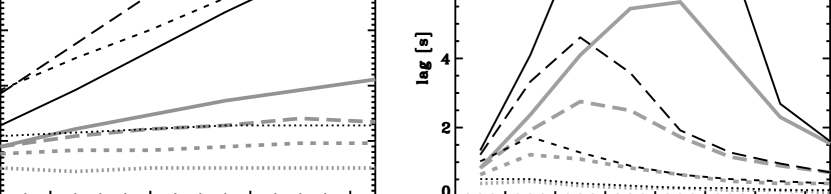
Figure 2: (a) Spectral lag as a function of pulse decay time scale, $\tau$, showing near-to linear relations. The parameters determining the spectral evolution were $E_{\rm 0}=500$ keV, $t_{\rm r}=1$ s, $\alpha=0$ (black lines) and $\alpha=-0.5$ (grey lines). The HIC power-law index ($d\,{\rm log}F/d\,{\rm log}E_{\rm p}$) $\eta=1.3$ (solid), $\eta=1.5$ (long dashed), $\eta=1.7$ (short dashed), $\eta=2.1$ (dotted). (b) Spectral lag as a function of $\eta$. Here $E_{\rm 0}=500$ keV, $t_{\rm r}=1$ s, $\tau=5.5$ s (black) and $\tau=2.5$ s (grey). The low-energy power-law index, $\alpha=0.5$ (solid), $\alpha=0.0$ (long dashed), $\alpha=-0.5$ (short dashed) and $\alpha=-1.0$ (dotted).

Figure 3: Contour plots of the spectral lag as a function of the HIC power-law index, $\eta$ and the spectral, low-energy, power-law, $\alpha$ for varying values of $E_{\rm 0}$: (a) $E_{\rm 0}=100$ keV, (b) $E_{\rm 0}=250$ keV, (c) $E_{\rm 0}=500$ keV, (d) $E_{\rm 0}=750$ keV.

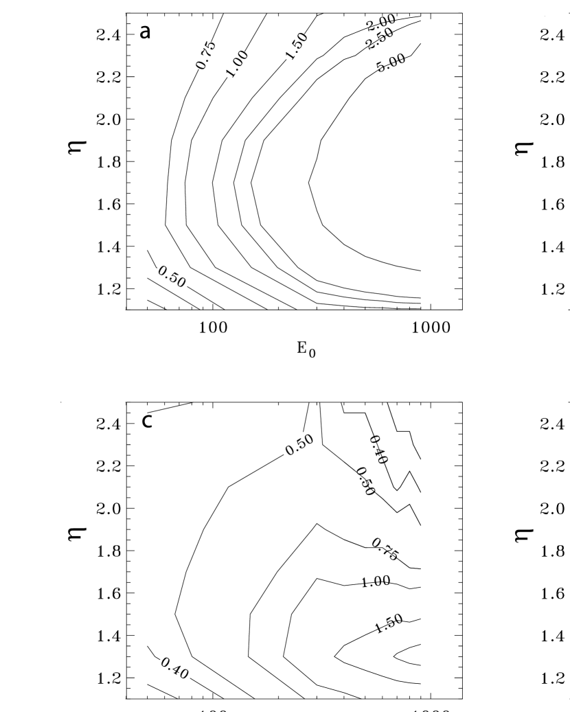
Figure 4: Contour plots of the spectral lag as a function of the HIC power-law index, $\eta$ and the energy $E_{0}$, for varying values of $\alpha$: (a) $\alpha=0.5$, (b) $\alpha=0.0$, (c) $\alpha=-0.5$, (d) $\alpha=-1.0$. These plots correspond to the black lines in Fig. 2b.

Kocevski, Ryde, & Liang (2003) expanded the analytical study of the pulse shape, made above, to also include the rise phase. We review this treatment here as we will make use of their result in the numerical simulations. As the evolution of $E_{\rm p}$ is still from hard to soft during the main part of the rise phase of a pulse, the energy flux and the $E_{\rm p}$ are anti-correlated during this phase. By arguing from physical first principles Kocevski et al. (2003) studied several analytical shapes for the whole pulse that includes the rise phase and asymptotically approaches Eq. (12) in the decay phase (which is the behavior we are interested in here). In most physical models both the peak of the energy spectrum and the luminosity are proportional to the random Lorentz factor of the shocked electrons to some power: $E_{\rm p}(t)\propto\Gamma_{\rm r}^{a}(t)\cdot g(t)$, and $F_{\rm E}(t)\propto\Gamma_{\rm r}^{b}(t)\cdot h(t).$ The functions $g(t)$ and $h(t)$ parameterize the unknown time dependence on particle densities, optical depth, magnetic field, kinematics, etc. The correlation between hardness and the energy flux can thus be described as

$$F_{\rm E}(t)\propto E_{\rm p}^{\gamma}\cdot f(t)$$ (23)

with $\gamma=b/a$ and $f(t)=h(t)g(t)^{-\gamma}$. During the decay phase of a pulse the power-law relation dominates the HIC, as in Eq.[1], whereas during the rise phase it will be dominated by the unknown function $f(t)$. It is reasonable to assume that the rise phase is connected to some transient process, for instance, an initial decrease in optical depth, increase in the number of energized particles, or the merging (or crossing) of two shells. After this initial phase, the original decay behavior as described by Eqs. (12) and (13) should emerge. We therefore use the following prescription

$$f(t)\propto 1-e^{-t/t_{\rm r}}$$ (24)

where the time constant $t_{\rm r}$ now represents the rise phase. This corresponds to $h(t)\propto g(t)^{\gamma}$ as $t>>t_{\rm r}$ and the function reaches the power law in Eq.(1) asymptotically. A few new parameters have to be introduced; the energy flux, the peak energy, and the time of the peak of the light curve, $F_{\rm m}$, $E_{\rm m}$, and $t_{\rm m}$:

$$F=F_{\rm m}\left(\frac{E_{\rm p}}{E_{\rm m}}\right)^{\gamma}\frac{1-e^{-t/t_{\rm r}}}{1-e^{-t_{\rm m}/t_{\rm r}}}$$ (25)

which, combined with the HFC (Eq.[3]), gives the differential equation governing the spectral and temporal evolution of the pulse. It has the following solution (see Kocevski et al. (2003) for details).

$$F(t)=\frac{A_{0}(1-e^{-t/t_{\rm r}})}{(1+(t+t_{\rm r}e^{-t/t_{\rm r}})/\tau)^{d}}$$ (26)

$$E_{\rm p}(t)=\frac{A_{1}}{(1+(t+t_{\rm r}e^{-t/t_{\rm r}})/\tau)^{(d-1)}}$$ (27)

where $A_{0}$ and $A_{1}$ are analytical functions of $d,\tau,t_{\rm r},\Phi_{\rm 0},F_{\rm m},E_{\rm m}$ and $t_{\rm m}$ and the decay index $d$ is defined by requiring that $F(t)\rightarrow t^{-d}$ as $t\rightarrow\infty$, which gives $\eta=d/(d-1)$. We introduce the peak energy at $t=0$, $E_{\rm 0}$ which gives $A_{1}=E_{\rm 0}(1+t_{\rm r}/\tau)^{(1/\eta-1)}$. The value of the flux at $t=0$ is arbitrary and is not important. The parameter $d$ is found to be about 2-3 (Kocevski et al., 2003).

The instantaneous photon spectrum is modelled by the standard GRB model (Band et al. (1993)), which is essentially a low-energy power-law, $F\propto E^{\alpha}$ exponentially connected to a high-energy power-law $F\propto E^{\beta}$ where the photon indices $\beta<\alpha$. In an $EF_{\rm E}$ representation the spectrum peaks at $E_{\rm p}$. The value of $\beta$ was kept constant throughout the analysis here, since we concentrate our efforts to study the dependence of the lag on $\alpha$.

To be able to study spectral lags, the light curves for the four BATSE channels were found by integrating the spectra over the respective bands. Normally, the energy edges vary somewhat from observation to observation. For the simulation we used typical, average values: $E_{1}=24$ keV, $E_{2}=60$ keV, $E_{3}=108$ keV, $E_{4}=10000$ keV. The spectral lag was then found by measuring the time between the peaks of the light curves in channel 3 and channel 1. The parameters that are used as input to the numerical analysis are the following: the maximal peak energy $E_{0}$, $F_{0}$, the low- and high-energy power laws, $\alpha$ and $\beta$, the HIC index $\eta$, the decay- and rise- time scales, $\tau$ and $t_{\rm r}$.

4.2 Spectral lags

The solid lines in Fig. 2a show the spectral lag, $\Delta t$, as a function of the decay time scale $\tau$ with $\alpha=0$, and for four different values of $\eta=1.3,1.5,1.7,$ and $2.1$. The dashed lines show the corresponding behavior for $\alpha=-0.5$. For both cases, $E_{\rm 0}=500$ keV and $t_{\rm r}=1$ s. The relation between $\Delta t$ and $\tau$ is approximately linear (except for the case of $\eta=2.1$, where a maximal value is reached). This shows that the lag is closely related to the decay timescale of the pulse. This is in agreement with the analytical results in the previous section.

The dependence of the spectral lag with the HIC power-law index, $\eta$, is shown in Fig. 2b, for four different values of $\alpha=0.5,0.0,-0.5,-1.0$. The solid curves are for $\tau=5.5$ s and the dashed are for $\tau=2.5$ s. Again $E_{\rm 0}=500$ keV and $t_{\rm r}=1$ s. The lag has a maximal value for a certain $\eta$-value, which increases for increasing $\alpha$. This illustrates the complexity of the interpretation of the spectral lag: a certain lag does not uniquely correspond to a $\eta$ value. The longer decay time compared to the rise time does not change the general behavior, it merely moves the curves to larger lags and larger $\eta$-values.

A more general picture of the dependence is given in the two following figures. In Fig. 3 the contour plots of $\Delta t$ is shown as a function of the HIC index, $\eta$, and $\alpha$. The largest values are found for hard spectra (large $\alpha$) and averaged HIC slopes. An increase in $E_{\rm 0}$, increases the lag values mainly for the hardest spectra. Fig. 2b represents slices of these contours. The corresponding plots with a dependence on the maximal energy, $E_{\rm 0}$ is shown in Fig. 4 for $\alpha=0.5,0.0,-0.5$ and $-1.0$ (left to right). Both Figs. 3 and 4 are for a pulse with $t_{\rm r}=1$ s and $\tau=5.5$. As $\alpha$ becomes softer (decreases) the lag, for a certain $\eta$ and $E_{\rm 0}$, decreases. Also the maximal value occurs for smaller and smaller $\eta$ values. We have made similar runs with varying pulse asymmetry, that is, varying the ratio of the rise and decay time-scales. As the decay time-scale, $\tau$, increases relative to $t_{\rm r}$, the contour plots have in general a similar form except near the maximal value of the lag, that is, the peak of the contour plot. The peak increases and becomes more accentuated while the parameter space away from the peak is constant.

4.3 Hardness Ratios

We also studied the dependence of the hardness ratio (HR) on varying $E_{\rm 0}$, $\eta$, and $\alpha$ over a single pulse. We simulated pulses and calculated the integrated photon flux in BATSE channels 1 and 3, over the interval of the pulse which was brighter than 0.1 of the peak flux. The ratio of these fluxes is defined as HR31. The results for a pulse with a rise time of 0.5 s and decay time of 2 s are depicted in the following three figures. Panel (a) in Fig. 5 shows the contour plots of the HR as a function of $\eta$ and $E_{0}$ while $\alpha$ was fixed and set to 0.0. For low values of $E_{0}$ the HR13 is practically independent of $\eta$ and is thus mainly determined by $E_{0}$. This is the case in particular for large $\eta$. A corresponding behavior is seen in panel (b) which shows the HR31 contours as a function of $\alpha$ and $E_{0}$. Here $\eta$ was fixed instead and set to 2.0. The hardness ratio HR13 is practically independent of $\alpha$ for low values of $E_{0}$, most clearly pronounced for the hardest spectra. The strongest dependence of the HR is therefore on $E_{\rm 0}$.

Often the relationship between the HR and the spectral lag is investigated and such plots are often used in LRS work (see, e.g., Fig. 4 in Norris, Marani, & Bonnell (2000)). In panel (a) in Fig. 6 the HR31 is plotted versus lag for a run with $\alpha$ set to 0.0. The data points are connected for constant $E_{0}$, with $E_{0}=1000$ for the curve furthest to the right and $E_{0}=100$ for the curve furthest to the left. The index $\eta$ increases upwards in the figure, along the curves, from $\eta=1.2$ to $\eta=3.1$. For low $E_{0}$ the hardness ratio is seen to be practically constant, independent of $\eta$, consistent with Fig. 5a. For large $\eta$-values the dependence of HR on lag becomes greater (the vertical section of the curves). The large change of the lag as $\eta$ varies for a constant $E_{\rm 0}$ is also caught by Fig. 4b, as discussed above. In panel (b) the HR31–spectral lag relations are shown for varying $\alpha$ with $\eta$ set to 2.0. The relations are approximate power-laws. This is consistent with previous figures; in Figs. 3, for a constant $\eta=2$ and $E_{0}$, the lag has a monotonic increase as a function of $\alpha$, while in Fig. 5b, again with $\eta=2$ and a constant $E_{0}$, we see that the HRs as a function of $\alpha$ will have a monotonic increase, or will be constant (independent). Hence the correlations in panel Fig. 6b. Here, a larger $E_{\rm 0}$ corresponds to a power-law at higher HR31 and the spectra get harder (larger $\alpha$) to the right in the figure. Again, for low $E_{\rm 0}$ values, the hardness ratio is independent of variations in lag. The HR31 and $E_{0}$ are correlated which can be seen in Fig. 5a and b. Among others, Band et al. (2004) have shown that such a relation exists observationally between $E_{\rm p}$ and the hardness ratio. This is shown in more detail in Fig. 7, which is from the same run as Fig. 5a; $\eta$ increases upwards, from $\eta=1.2$ to $\eta=3.1$. The dispersion, introduced by a variation in $\eta$, is thus largest for large values of $E_{\rm 0}$.

Figure 5: Hardness ratio dependence on $\eta$, $\alpha$, and $E_{0}$, shown as contour plots. In panel (a) $\alpha=0$, while in (b) $\eta=2.0$. Note that the HR is practically independent of both $\eta$ and $\alpha$ at low energies.

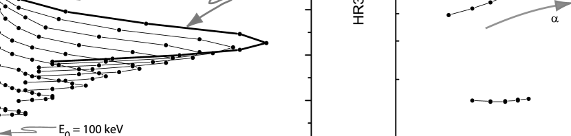
Figure 6: Hardness ratio as a function of spectral lag. In panel (a) each curve is for a certain $E_{\rm 0}$, with the thick line representing the largest value; $\eta$ increases upwards along the lines. Similarly, in panel (b), $E_{\rm 0}$ increases upwards for each curve and $\alpha$ increases to the right along each curve. In panel (a) $\alpha=0$, and (b) $\eta=2.0$.

Figure 7: The dependence of the hardness ratio $HR31$ on the peak energy $E_{0}$, for the same run as in Fig. 5a. Each curve is for a different $\eta$, increasing upwards in the figure, from $\eta=1.2$ to $3.1$. A variation in $\eta$ will thus lead to a dispersion, which becomes larger for higher $E_{\rm 0}$-values.

5 Discussion

The above numerical work has presented the somewhat complex expression that the spectral evolution has in the two observables, namely the spectral lag and the hardness ratio. The results can be used to interpret lag and HR observations of various burst samples.

5.1 Interpretation

The dependence of the lag on $\alpha$ is given in Fig. 3. It shows that the lag increases with $\alpha$ for all tested values on $\eta$. The more energetic the pulses/bursts are (higher $E_{\rm 0}$) the steeper this correlation will be. Furthermore, the size of the lags can give a hint of the hardness of the spectra: a hard spectrum, for instance a thermal spectrum ($\alpha=+1$) or a small pitch-angle synchrotron-spectrum ($\alpha=0$), will have a larger lag than a corresponding softer spectrum, maybe produced by optically-thin synchrotron emission ($\alpha=-2/3,-3/2$). Figure 3 also shows that, if a sample of spectrally hard pulses (large $\alpha$) is chosen, then the plot between lag and $\eta$ will have a characteristic bump indicating the distribution of $E_{\rm 0}$ in the sample studied. Note that each panel in Fig. 3 corresponds to a specific $E_{\rm 0}$-value. A softer sample will have a less pronounced dependence (compare Fig. 2b).

Furthermore, by studying the lag as a function of $E_{\rm 0}$, for a sample of bursts, conclusions can be drawn using the information available in Fig. 4. For instance, if the lag is found to increase with $E_{\rm 0}$, the sample is probably dominated by hard pulses, or at least do not have particularly large $\eta$-values. Oppositely, the lag could be found to decrease with $E_{\rm 0}$. This could indicate that the sample is dominated by soft spectra (panel d; especially at high energies). For harder spectra, such a decline is found only in pulses with the very largest $\eta$. Continuing with Fig. 4, we see that if, once again, lag is plotted versus $\eta$ and only a weak dependence is found, the pulses are most probably low-energetic bursts, such as X-ray flashes. This is so especially in the case of soft spectral pulses (compare Fig. 3). For high-energetic bursts (high $E_{\rm 0}$) the characteristic dependence, with a peak at some intermediate $\eta$, will be seen and the range of observed lags will be large. For very soft pulses (small $\alpha$) it will mainly be a declining function. Note that the panels in the figure are for constant $\alpha$-values. Correlations between, for instance, $\eta$ and $\alpha$ in the sample under investigation will complicate the interpretation slightly, since the same panel cannot be used for all $\eta$. Also, since there are different possible dependence, the distribution of $E_{\rm 0}$ of the sample will be important in determining the final relation.

Similarly, differences in HIC-index $\eta$ between samples will be marked by that the hardness ratio generally is largest for the large–$\eta$ pulses (except for very low $E_{\rm 0}$). This is for instance manifested in Fig. 7 in which the large–$\eta$ pulses have a steeper dependence on the peak energy. The largest lags are found for pulses with intermediate $\eta\sim 1.5$ – $\eta\sim 2$. As mentioned above, soft burst will have a characteristic switch in lag versus $E_{\rm 0}$ behavior, from increasing (for low $\eta$) to decrease (for large $\eta$).

Figures 5, 6 and 7 reflect the behavior of the hardness ratios. If, for instance, the HR is plotted versus $\alpha$ ($\eta$) and the relations are found to be weak, it is again an indication of low-energetic bursts. The distribution of the pulses in the HR-lag–plane will give indications of both $E_{\rm 0}$ and $\eta$ according to the plot.

5.2 Radiation processes and emission sites

Several different emission mechanisms are probably active during the burst (see e.g. Ryde 2004), most importantly various versions of synchrotron (and/or inverse Compton) emission, predominantly its optically-thin version, and thermal, black-body emission. Other possible radiation mechanisms include synchrotron emission from electrons with a small pitch-angle distribution (or jitter radiation) and saturated Comptonization. The most visible difference is in the hardness of the spectra, as measured by the low-energy power-law index $\alpha$. A certain sample of bursts can thus be studied with the relations discussed above, to discern the dominating radiation process. For instance, on the basis of the durations and hardnesses, bursts seem to belong to two distinct classes (e.g. Balázs et al. (2003)), or even three (Horváth, 1998; Horváth et al., 2004). Any difference in radiation mechanism between these classes can therefore be efficiently investigated.

It is also known that the importance of the curvature effect varies between pulses (see e.g. Ryde & Petrosian (2002)). In the case of it being important, the HIC index, $\eta$, will have a characteristic behavior and a large value. In Fig. 5a, $\eta=3$ for a curvature-driven pulse is marked by the dashed line and the relation between HR31 and spectral lags for such pulses is shown in Fig. 8. This shows the hardness ratio decreasing linearly with the corresponding time lag. In this particular run $\alpha=-0.5$. $E_{0}$ decreases to the right with the point furthest to the left with $E_{0}=1000$ keV and the point furthest to the right with $E_{0}=100$ keV. This decrease is obvious in Fig. 4, in which large values of $\eta$ and soft spectra sample a space where the lag decreases with $E_{0}$. This, together with the positive correlation between $E_{\rm 0}$ and HR31 depicted in Fig. 7, then gives the relation in Fig. 8. On the other hand, if the dominant time-scale is not the curvature time-scale then the intrinsic $\eta$, representing the comoving radiation process, will be revealed. For instance, assuming synchtroton emission and a constant bulk Lorentz factor, $\Gamma$, we expect $E_{\rm p}\propto\gamma^{2}_{min}\cdot B$ (the minimum electron Lorentz factor and the magnetic field strength) and $F\propto{\cal E}_{e}\cdot B^{2}\cdot\gamma_{min}$, where ${\cal E}_{e}=\int_{0}^{\infty}\gamma N(\gamma)d\gamma$ is the total electron energy ($N(\gamma)$ is the energy spectrum of electrons). If the latter quantity is constant, we expect $\eta=2$ if $B$ varies and $\gamma_{min}$ is constant and $\eta=1/2$ if $B$ is constant and $\gamma_{min}$ varies. The observed correlations would then sample different regions in the panels discussed above.

Figure 8: Correlation between hardness ratio and spectral lag for a ”curvature-driven” pulse ($\eta=3$). $E_{\rm 0}$ decreased to the right. See the text for further details.

During the past few years increasing numbers of X-ray rich GRBs and so-called X-ray flashes (XRF) have been observed (Heise et al. 2000, Barraud et al. 2003). Several studies have shown that the main difference in properties between these populations and classical GRBs is the peak energy distribution. It has therefore been suggested that they are all of the same origin (e.g. Kippen et al., 2002, 2003, Lamb et al., 2004) and that XRF is an extension of the GRB energy distribution. As described above the distribution of peak energy between different samples will have characteristic signatures on the lag correlations and can be further used in studying the difference between GRBs and XRFs.

6 Conclusion

The two spectroscopical analysis methods discussed in this paper, HRS and LRS measure the same underlying behavior and are alternative ways to represent the spectral evolution. We have shown analytically and numerically that the spectral evolution described by high spectral-resolution data, in empirical correlations, naturally leads to correlations involving spectral lags. The interpretation of the spectral lag is not straightforward. This depends on the fact that the lag measures a combination of spectral parameters such as $\eta$, $E_{\rm 0}$, and $\tau$ (apart from effects caused by $\alpha$ and $\beta$; their values and evolution). It further depends on the relative channel widths into which the data are divided. For different pulses within a burst, the spectral parameters are in general not the same, and thus the lag is not expected to be the same during the whole burst. This is indeed the case in observed bursts, as we note in paper II (Ryde et al. 2004).

The main result of the above analysis is that the lag correlates strongly with the decay time-scale of the pulse (or equivalently, of the peak-energy decay) and that this relation is linear. This means that the relationships including the lag, that have been identified, should be translatable into relationships including the pulse time-scale. This time-scale is closely connected to the processes forming the pulse in the out-flowing plasma; the radiation processes, acceleration mechanisms, light-travel effects and outflow velocity etc. In particular, we find a good correlation between lag and the quantity $F/\Phi_{0}$, reproducing the observation by Kocevski & Liang (2003b). We further find that harder spectra, with large $\alpha$, have the largest spectral lags. This is, in particular, the case for averaged $\eta$–values. Similarly, an increase in $E_{\rm 0}$, increases the lag, except for soft $\alpha$ (see Fig.4 d). Interestingly, the hardness ratio is found to be only weakly dependent on $\eta$ and $\alpha$, and in particular for low, initial peak energies $E_{\rm 0}$ it is practically independent, and it is mainly determined by $E_{\rm 0}$; according to Fig. 6a. The relation between the hardness ratio and the lags, for a certain $E_{\rm 0}$ and $\eta$, are described by power-laws, as $\alpha$ varies (Fig. 5d). Furthermore, for a curvature-driven pulse ($\eta=3$), the hardness ratio decreases linearly with lag for lower and lower $E_{\rm 0}$.

The analytical and numerical results presented here are the consequences of the empirical description of the spectral evolution in pulses, which have been firmly established. These results can thus be used as a reference in the analysis of observed pulses and bursts, in particular low spectral-resolution studies in which the spectral parameters cannot be found and mainly the lag and hardness ratios are analyzed. Such an analysis is performed in paper II (Ryde et al. 2004) in which we also discuss how the conclusions presented here relate to the physical models that have been proposed to explain the observed lag-correlations.