COSMOLOGICAL THEORIES OF SPECIAL AND GENERAL RELATIVITY - II

Moshe Carmeli ^a

^a Department of Physics, Ben Gurion University of the Negev, Beer Sheva 84105, Israel

Abstract

Astronomers measure distances to faraway galaxies and their velocities. They do that in order to determine the expansion rate of the Universe. In Part I of these lectures the foundations of the theory of the expansion of the Universe was given. In this part we present the theory. A formula for the distance of the galaxy in terms of its velocity is given. It is very simple: $r(v)=c\tau/\beta\sinh\beta v/c$, where $\tau$ is the Big Bang time, $\beta=\sqrt{1-\Omega_{m}}$, and $\Omega_{m}$ is the mass density of the Universe. For $\Omega_{m}<1$ this formula clearly indicates that the Universe is expanding with acceleration, as experiments clearly show.

1 Gravitational field equations

In the four-dimensional spacevelocity the spherically symmetric metric is given by

$$ds^{2}=\tau^{2}dv^{2}-e^{\mu}dr^{2}-R^{2}\left(d\theta^{2}+\sin^{2}\theta d\phi^{2}\right),$$

where $\mu$ and $R$ are functions of $v$ and $r$ alone, and comoving coordinates $x^{\mu}=(x^{0},x^{1},x^{2},x^{3})=(\tau v,r,\theta,\phi)$ have been used. With the above choice of coordinates, the zero-component of the geodesic equation becomes an identity, and since $r$, $\theta$ and $\phi$ are constants along the geodesics, one has $dx^{0}=ds$ and therefore $u^{\alpha}=u_{\alpha}=\left(1,0,0,0\right).$ The metric (1.1) shows that the area of the sphere $r=constant$ is given by $4\pi R^{2}$ and that $R$ should satisfy $R^{\prime}=\partial R/\partial r>0$. The possibility that $R^{\prime}=0$ at a point $r_{0}$ is excluded since it would allow the lines $r=constants$ at the neighboring points $r_{0}$ and $r_{0}+dr$ to coincide at $r_{0}$, thus creating a caustic surface at which the comoving coordinates break down.

As has been shown in Part I the Universe expands by the null condition $ds=0$, and if the expansion is spherically symmetric one has $d\theta=d\phi=0$. The metric (1.1) then yields $\tau^{2}dv^{2}-e^{\mu}dr^{2}=0,$ thus

$$\frac{dr}{dv}=\tau e^{-\mu/2}.$$

This is the differential equation that determines the Universe expansion. In the following we solve the gravitational field equations in order to find out the function $\mu\left(r.v\right)$.

The gravitational field equations, written in the form

$$R_{\mu\nu}=\kappa\left(T_{\mu\nu}-g_{\mu\nu}T/2\right),$$

where

$$T_{\mu\nu}=\rho_{eff}u_{\mu}u_{\nu}+p\left(u_{\mu}u_{\nu}-g_{\mu\nu}\right),$$

with $\rho_{eff}=\rho-\rho_{c}$ and $T=T_{\mu\nu}g^{\mu\nu}$, are now solved. One finds that the only nonvanishing components of $T_{\mu\nu}$ are $T_{00}=\tau^{2}\rho_{eff}$, $T_{11}=c^{-1}\tau pe^{\mu}$, $T_{22}=c^{-1}\tau pR^{2}$ and $T_{33}=c^{-1}\tau pR^{2}\sin^{2}\theta$, and that $T=\tau^{2}\rho_{eff}-3c^{-1}\tau p$.

One obtains three independent field equations (dot and prime denote derivatives with $v$ and $r$)

$$e^{\mu}\left(2R\ddot{R}+\dot{R}^{2}+1\right)-R^{\prime 2}=-\kappa\tau c^{-1}e^{\mu}R^{2}p,$$

$$2\dot{R}^{\prime}-R^{\prime}\dot{\mu}=0,$$

$$e^{-\mu}\left[\frac{1}{R}R^{\prime}\mu^{\prime}-\left(\frac{R^{\prime}}{R}\right)^{2}-\frac{2}{R}R^{\prime\prime}\right]+\frac{1}{R}\dot{R}\dot{\mu}+\left(\frac{\dot{R}}{R}\right)^{2}+\frac{1}{R^{2}}=\kappa\tau^{2}\rho_{eff}.$$

2 Solution of the field equations

The solution of (1.6) satisfying the condition $R^{\prime}>0$ is given by

$$e^{\mu}=R^{\prime 2}/\left(1+f\left(r\right)\right),$$

where $f\left(r\right)$ is an arbitrary function of the coordinate $r$ and satisfies the condition $f\left(r\right)+1>0$. Substituting (2.1) in the other two field equations (1.5) and (1.7) then gives

$$2R\ddot{R}+\dot{R}^{2}-f=-\kappa c^{-1}\tau R^{2}p,$$

$$\frac{1}{RR^{\prime}}\left(2\dot{R}\dot{R^{\prime}}-f^{\prime}\right)+\frac{1}{R^{2}}\left(\dot{R}^{2}-f\right)=\kappa\tau^{2}\rho_{eff},$$

respectively.

The simplest solution of the above two equations, which satisfies the condition $R^{\prime}=1>0$, is given by $R=r$. Using this in Eqs. (2.2) and (2.3) gives $f\left(r\right)=\kappa c^{-1}\tau pr^{2}$, and $f^{\prime}+f/r=-\kappa\tau^{2}\rho_{eff}r$, respectively. Using the values of $\kappa=8\pi G/c^{2}\tau^{2}$ and $\rho_{c}=3/8\pi G\tau^{2}$, we obtain

$$f\left(r\right)=\left(1-\Omega_{m}\right)r^{2}/c^{2}\tau^{2},$$

where $\Omega_{m}=\rho/\rho_{c}$. We also obtain

$$p=\frac{1-\Omega_{m}}{\kappa c\tau^{3}}=\frac{c}{\tau}\frac{1-\Omega_{m}}{8\pi G}=4.544\left(1-\Omega_{m}\right)\times 10^{-2}g/cm^{2},$$

$$e^{-\mu}=1+f\left(r\right)=1+\tau c^{-1}\kappa pr^{2}=1+\left(1-\Omega_{m}\right)r^{2}/c^{2}\tau^{2}.$$

Accordingly, the line element of the Universe is given by

$$ds^{2}=\tau^{2}dv^{2}-\frac{dr^{2}}{1+\left(1-\Omega\right)r^{2}/c^{2}\tau^{2}}-r^{2}\left(d\theta^{2}+\sin^{2}\theta d\phi^{2}\right),$$

or,

$$ds^{2}=\tau^{2}dv^{2}-\frac{dr^{2}}{1+\left(\kappa\tau/c\right)pr^{2}}-r^{2}\left(d\theta^{2}+\sin^{2}\theta d\phi^{2}\right).$$

This line element is the comparable to the FRW line element in the standard theory.

It will be recalled that the Universe expansion is determined by Eq. (1.2), $dr/dv=\tau e^{-\mu/2}$. The only thing that is left to be determined is the sign of $(1-\Omega_{m})$ or the pressure $p$. Thus we have

$$\frac{dr}{dv}=\tau\sqrt{1+\kappa\tau c^{-1}pr^{2}}=\tau\sqrt{1+\frac{1-\Omega_{m}}{c^{2}\tau^{2}}r^{2}}.$$

3 Physical meaning

For $\Omega_{m}>1$ one obtains

$$r\left(v\right)=\frac{c\tau}{\alpha}\sin\alpha\frac{v}{c},\hskip 14.22636pt\alpha=\sqrt{\Omega_{m}-1}.$$

This is obviously a closed Universe, and presents a decelerating expansion.

For $\Omega_{m}<1$ one obtains

$$r\left(v\right)=\frac{c\tau}{\beta}\sinh\beta\frac{v}{c},\hskip 14.22636pt\beta=\sqrt{1-\Omega_{m}}.$$

This is now an open accelerating Universe.

For $\Omega_{m}=1$ we have, of course, $r=\tau v$.

4 The accelerating Universe

From the above one can write the expansion of the Universe in the standard Hubble form $v=H_{0}r$ with

$$H_{0}=h\left[1-\left(1-\Omega_{m}\right)v^{2}/6c^{2}\right],$$

where $h=\tau^{-1}$. Thus $H_{0}$ depends on the distance it is being measured [12]. It is well-known that the farther the distance, the lower the value for $H_{0}$ is measured. This is possible only for $\Omega_{m}<1$, i.e. when the Universe is accelerating. In that case the pressure is positive.

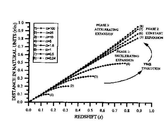
Figure 1 describes the Hubble diagram of the above solutions for the three types of expansion for values of $\Omega_{m}$ from 100 to 0.245. The figure describes the three-phase evolution of the Universe. Curves (1)-(5) represent the stages of decelerating expansion according to Eq. (3.1). As the density of matter $\rho$ decreases, the Universe goes over from the lower curves to the upper ones, but it does not have enough time to close up to a Big Crunch. The Universe subsequently goes over to curve (6) with $\Omega_{m}=1$, at which time it has a constant expansion for a fraction of a second. This then followed by going to the upper curves (7) and (8) with $\Omega_{m}<1$, where the Universe expands with acceleration according to Eq. (3.2). Curve no. 8 fits the present situation of the Universe. For curves (1)-(4) in the diagram we use the cutoff when the curves were at their maximum.

Figure 1: Hubble’s diagram describing the three-phase evolution of the Universe according to cosmological general relativity theory.

5 Theory versus experiment

To find out the numerical value of $\tau$ we use the relationship between $h=\tau^{-1}$ and $H_{0}$ given by Eq. (4.1)(CR denote values according to Cosmological Relativity):

$$H_{0}=h\left[1-\left(1-\Omega_{m}^{CR}\right)z^{2}/6\right],$$

where $z=v/c$ is the redshift and $\Omega_{m}^{CR}=\rho_{m}/\rho_{c}$ with $\rho_{c}=3h^{2}/8\pi G$. (Notice that our $\rho_{c}=1.194\times 10^{-29}g/cm^{3}$ is different from the standard $\rho_{c}$ defined with $H_{0}$.) The redshift parameter $z$ determines the distance at which $H_{0}$ is measured. We choose $z=1$ and take for $\Omega_{m}^{CR}=0.245$, its value at the present time (corresponds to 0.32 in the standard theory), Eq. (5.1) then gives $H_{0}=0.874h.$ At $z=1$ the corresponding Hubble parameter $H_{0}$ according to the latest results from HST can be taken [20] as $H_{0}=70$km/s-Mpc, thus $h=(70/0.874)$km/s-Mpc, or $h=80.092\mbox{\rm km/s-Mpc},$ and $\tau=12.486Gyr=3.938\times 10^{17}s.$

What is left is to find the value of $\Omega_{\Lambda}^{CR}$. We have $\Omega_{\Lambda}^{CR}=\rho_{c}^{ST}/\rho_{c}$, where $\rho_{c}^{ST}=3H_{0}^{2}/8\pi G$ and $\rho_{c}=3h^{2}/8\pi G$. Thus $\Omega_{\Lambda}^{CR}=(H_{0}/h)^{2}=0.874^{2}$, or $\Omega_{\Lambda}^{CR}=0.764.$ As is seen from the above equations one has

$$\Omega_{T}=\Omega_{m}^{CR}+\Omega_{\Lambda}^{CR}=0.245+0.764=1.009\approx 1,$$

which means the Universe is Euclidean.

Our results confirm those of the supernovae experiments and indicate on the existance of the dark energy as has recently received confirmation from the Boomerang cosmic microwave background experiment [21, 22], which showed that the Universe is Euclidean.

6 Comparison with general relativity

One has to add the time coordinate and the result is a five-dimensional theory of space-time-velocity. One can show that all the classical experiments predicted by general relativity are also predicted by CGR. Also predicted a wave equation for gravitational radiation. In the linear approximation one obtains

$$\left(\frac{1}{c^{2}}\frac{\partial^{2}}{\partial t^{2}}-\nabla^{2}+\frac{1}{\tau^{2}}\frac{\partial^{2}}{\partial v^{2}}\right)\gamma_{\mu\nu}=-2\kappa T_{\mu\nu},$$

where $\gamma_{\mu\nu}$ is a first approximation term,

$$g_{\mu\nu}\approx\eta_{\mu\nu}+h_{\mu\nu}=\eta_{\mu\nu}+\gamma_{\mu\nu}-\eta_{\mu\nu}\gamma/2,$$

$$\gamma=\eta^{\alpha\beta}\gamma_{\alpha\beta}.$$

Hence CGR predicts that gravitational waves depend not only on space and time but also on the redshift of the emitting source.

	COSMOLOGICAL	STANDARD
	RELATIVITY	THEORY
Theory type	Spacevelocity	Spacetime
Expansion	Tri-phase:	One phase
type	decelerating, constant,
	accelerating
Present expansion	Accelerating	One of three
	(predicted)	possibilities
Pressure	$0.034g/cm^{2}$	Negative
Cosmological constant	$1.934\times 10^{-35}s^{-2}$	Depends
	(predicted)
$\Omega_{T}=\Omega_{m}+\Omega_{\Lambda}$	1.009	Depends
Constant-expansion	8.5Gyr ago	No prediction
occurs at	(Gravity is included)
Constant-expansion	Fraction of	Not known
duration	second
Temperature at	146K	No prediction
constant expansion	(Gravity is included)

Table 1: Cosmological parameters in cosmological general relativity and in standard theory.

7 New developments on dark matter

Using the theory presented here, John Hartnett has recently shown that there is no need for the existence of dark matter in spiral galaxies. We only give the references to this work by Hartnett [25, 26, 27].

References

- [1] M. Carmeli, Cosmological Special Relativity, 2nd Edition, World Scientific (2002)
- [2] M. Carmeli and T. Kuzmenko, ”Value of the cosmological constant”, astro-ph/0110590
- [3] M. Carmeli, Proc. 20th Texas Symp., AIP Conf. Proc., 586 (2001), astro-ph/012033
- [4] M. Carmeli, ”Accelerating Universe: Theory vs experiment”, astro-ph/0205396
- [5] M. Carmeli, ”Five-dimensional cosmological theory of unified space, time and velocity”, Nuclear Phys B124, 258 (2003); asrto-ph/0205113
- [6] M. Carmeli, ”The line element in the Hubble expansion”, In: Gravitation and cosmology, A. Lobo et al. Eds., Universitat de Barcelona, 2003, pp. 113-130 (Proceedings of the Spanish Relativity Meeting, Menorca, Spain, 22-24 September 2002); astro-ph/0211043
- [7] M. Carmeli, Commun. Theor. Phys. 5, 159 (1996)
- [8] M. Carmeli, Classical Fields: General Relativity and Gauge Theory, Wiley, New York (1982) [reprinted by World Scientific (2001)]
- [9] S. Behar and M. Carmeli, Intern. J. Theor. Phys. 39, 1375 (2000), astro-ph/0008352
- [10] M. Carmeli and S. Behar, ”Cosmological general relativity”, pp. 5-26, in: Quest for Mathematical Physics, T.M. Karade et al. Eds., New Delhi (2000)
- [11] M. Carmeli and S. Behar, ”Cosmological relativity: a general relativistic theory for the accelerating Universe”, Talk given at Dark Matter 2000, Los Angeles, February 2000, pp.182–191, in: Sources and Detection of Dark Matter/Energy in the Universe, D. Cline, Ed., Springer (2001)
- [12] P.J.E. Peebles, Status of the big bang cosmology, in: Texas/Pascos 92: Relativistic Astrophysics and Particle Cosmology, C.W. Akerlof and M.A. Srednicki, Editors, p. 84, New York Academy of Sciences, New York (1993)
- [13] P.M. Garnavich et al., Astrophys. J. 493, L53 (1998) [Hi-Z Supernova Team Collaboration (astro-ph/9710123)]
- [14] B.P. Schmidt et al., Astrophys. J. 507, 46 (1998) [Hi-Z Supernova Team Collaboration (astro-ph/9805200)]
- [15] A.G. Riess et al., Astronom. J. 116, 1009 (1998) [Hi-Z Supernova Team Collaboration (astro-ph/9805201)]
- [16] P.M. Garnavich et al., Astrophys. J. 509, 74 (1998) [Hi-Z Supernova Team Collaboration (astro-ph/9806396)]
- [17] S. Perlmutter et al., Astrophys. J. 483, 565 (1997) [Supernova Cosmology Project Collaboration (astro-ph/9608192)].
- [18] S. Perlmutter et al., Nature 391, 51 (1998) [Supernova Cosmology Project Collaboration (astro-ph/9712212)]
- [19] S. Perlmutter et al., Astrophys. J. 517, 565 (1999) [Supernova Cosmology Project Collaboration (astro-ph/9812133)]
- [20] W.L. Freedman et al., ”Final results from the Hubble Space Telescope”, Talk given at the 20th Texas Symposium on Relativistic Astrophysics, Austin, Texas 10-15 December 2000, (astro-ph/0012376)
- [21] P. de Bernardis et al., Nature 404, 955 (2000), (astro-ph/0004404)
- [22] J.R. Bond et al., in Proc. IAU Symposium 201 (2000), (astro-ph/0011378)
- [23] A.V. Filippenko and A.G. Riess, p.227 in: Particle Physics and Cosmology: Second Tropical Workshop, J.F. Nieves, Editor, AIP, New York (2000)
- [24] A.G. Riess et al., Astrophys. J., in press, astro-ph/0104455
- [25] J. Hartnett, ”Carmeli’s accelerating Universe is spatially flat without dark matter”, Intern. J. Theor. Phys., in press (accepted for publication) (2004), gr-qc/0407082
- [26] J. Hartnett, ”Can the Carmeli metric correctly describe spiral galaxy rotation curves?” 2004, gr-qc/0407083
- [27] J. Hartnett, ”Carmeli’s cosmology: The Universe is spatially flat without dark matter”, invited talk given at the international conference ”Frontiers of Fundamental Physics 6”, held in Udine, Italy, September 26-29, 2004