Extra-galactic magnetic fields and the second knee in the cosmic-ray spectrum

Abstract

Recent work suggests that the cosmic ray spectrum may be dominated by Galactic sources up to $\sim 10^{17.5}\,$eV, and by an extra-Galactic component beyond, provided this latter cuts off below the transition energy. Here it is shown that this cut-off could be interpreted in this framework as a signature of extra-galactic magnetic fields with equivalent average strength $B$ and coherence length $l_{\rm c}$ such that $B\sqrt{l_{\rm c}}\sim 2-3\cdot 10^{-10}\,$G$\cdot$Mpc^1/2, assuming $l_{\rm c}<r_{\rm L}$ (Larmor radius at $\lesssim 10^{17}\,$eV) and continuously emitting sources with density $10^{-5}\,$Mpc^-3. The extra-Galactic flux is suppressed below $\sim 10^{17}\,$eV as the diffusive propagation time from the source to the detector becomes larger than the age of the Universe.

I Introduction

Recent developments, both experimental and theoretical, have significantly broadened the landscape of ultra-high energy cosmic ray phenomenology. The High Resolution Fly’s Eye experiment has reported the detection of a high energy cut-off $\sim 10^{20}\,$eV HiRes , as would be expected from a cosmological population of sources. This experiment has also observed that the chemical composition is dominated by protons down to $\sim 10^{18}\,$eV, and by heavy nuclei further below, in agreement with preliminary KASCADE data KASCADE . This and the steepening of the cosmic-ray spectrum at the “second knee” $\sim 10^{17.5}\,$eV suggest the disappearance of the low-energy (heavy nuclei) component and the nearly simultaneous emergence of a high-energy (proton) component. On theoretical grounds, it has been observed by Berezinsky et al. BGG1 that a cosmological distribution of sources producing a single powerlaw could fit the high energy part of the cosmic-ray spectrum from the second knee up to the cut-off at $10^{20}\,$eV, including the dip of the ”ankle” $\sim 10^{18.5}$eV. In light of these results, it is thus tempting to think that the cosmic-ray spectrum consists of only two main components: one Galactic, another extra-galactic, with the transition around the second knee.

There are alternative views, admittedly, in which the Galactic component dominates the all-particle spectrum up the ankle WW04 ; this latter feature would then mark the emergence of the extra-galactic component rather than the signature of pair production as in Ref. BGG1 . This issue will be hopefully settled by ongoing and future cosmic ray experiments, through more accurate composition and anisotropy measurements. The discussion that follows assumes that the interpretation of Berezinsky and coworkers BGG1 is correct, namely, that the transition between the Galactic and extra-galactic cosmic ray component arises at the second knee.

This model then requires to impose a low-energy cut-off on the extra-galactic spectrum around $10^{18}\,$eV in order to not overproduce the flux close to the second knee. The exact position of this cut-off as well as the spectral slope below it must be tuned to how the Galactic component extends above the knee BGG2 .

The objective of the present work is to demonstrate that this cut-off could be interpreted as a signature of extra-galactic magnetic fields with average strength $B$ and coherence length $l_{\rm c}$ such that $B\sqrt{l_{\rm c}}\sim 2-3\cdot 10^{-10}\,$G$\cdot$Mpc^1/2, assuming $l_{\rm c}<r_{\rm L}$ Larmor radius at $\lesssim 10^{17}\,$eV and continuously emitting sources with density $10^{-5}\,$Mpc^-3. In this picture, the extra-Galactic spectrum shuts off below $10^{17}\,$eV as the diffusion time from the closest sources becomes larger than the age of the Universe. The first knee is viewed here as the maximal injection energy for protons at the (Galactic) source.

The existence of extra-galactic magnetic fields is of importance to various fields of astrophysics, including ultra-high energy cosmic ray phenomenology, but very little is known on their origin, on their spatial configuration and on their amplitude W03 . The upper limits on $B\sqrt{l_{\rm c}}$ from Faraday observations lie some two orders of magnitude above the value suggested here. In the present framework, experiments such as KASCADE-Grande KASCADE could probe these magnetic fields thanks to accurate measurements of the spectrum and composition in the range $10^{16}\rightarrow 10^{18}\,$eV.

II Particle propagation

The main effect of extra-galactic magnetic fields on $\sim 10^{17}\,$eV particles is as follows. In a Hubble time, these particles travel by diffusing on magnetic inhomogeneities a linear distance $d\sim\left(cH_{0}^{-1}l_{\rm scatt}\right)^{1/2}\simeq 65\,{\rm Mpc}\,(l_{\rm scatt}/1\,{\rm Mpc})^{1/2}$, with $l_{\rm scatt}$ the scattering length of the particle. If $d$ is much smaller than the typical source distance, the particle cannot reach the detector in a Hubble time; since $l_{\rm scatt}$, hence $d$, increases with increasing energy, this produces a low-energy cut-off in the propagated spectrum. Current data at the highest energies, notably the clustering seen by various experiments, suggests a cosmic-ray source density $n\sim 10^{-6}-10^{-5}\,$Mpc^-3 ns , which corresponds to a source distance scale $\sim 50-100\,$Mpc. Hence $l_{\rm scatt}\lesssim 0.3-1\,$Mpc at $10^{17}\,$eV would shut off the spectrum below this energy ILS01 .

To be more quantitative one has to calculate the propagated spectrum and compare it to the observed data. The low energy part ($\lesssim 10^{18}\,$eV in what follows) of the extra-galactic proton spectrum diffuses in the extra-galactic magnetic field since the scattering length $l_{\rm scatt}\ll d$ ($d$ typical source distance). In contrast, particles of higher energies ($\gtrsim 10^{19}\,$eV in what follows) travel in a quasi-rectilinear fashion, meaning that the total deflection angle $\theta_{\rm rms}\ll 1$, since $l_{\rm scatt}\gg l_{\rm loss}$, where $l_{\rm loss}\lesssim 1\,$Gpc at $E\gtrsim 10^{19}\,$eV is the energy loss length (which gives an upper bound to the linear distance across which particles can travel).

In the diffusion approximation, the propagated differential spectrum reads (see the Appendix):

$$J_{\rm diff}(E)\,=\,{c\over 4\pi}\int{\rm d}t\sum_{i}\,{e^{-r_{i}^{2}/(4\lambda^{2})}\over(4\pi\lambda^{2})^{3/2}}\,{{\rm d}E_{\rm g}(t,E)\over{\rm d}E}\,Q\left[E_{\rm g}(t,E)\right].$$ (1)

The sum carries over the discrete source distribution; $r_{i}$ is the comoving distance to source $i$. Note that a factor $(a_{0}/a_{\rm e})^{-3}$ in Eq. (4), with $a_{0}$ and $a_{\rm e}$ the scale factor at observation and emission respectively, has been absorbed in defining a comoving source density; the remaining factor $(a_{0}/a_{\rm e})\approx{\rm d}E_{\rm g}/{\rm d}E$, see below. The function $E_{\rm g}(t,E)$ defines the energy of the particle at time $t$, assuming it has energy $E$ at time $t_{0}$. This function and its derivative ${\rm d}E_{\rm g}/{\rm d}E$ can be reconstructed by integrating the energy losses BGG1 . In the Appendix, it is shown that Eq. (1) provides a solution to the diffusion equation in the expanding space-time under the assumption that the energy loss of the particle is dominated by expansion losses, which is found to be a good approximation for particles with observed energies $E\lesssim 10^{18}\,$eV. In this case, ${\rm d}E_{\rm g}/{\rm d}E\approx E_{\rm g}/E\approx a_{0}/a_{\rm e}$. Although photopair and photopion production losses on diffuse backgrounds are negligible with respect to expansion losses for most of the particle history, they set the maximum linear distance (hence the maximum time) across which a particle can travel. The time integral in Eq.(1) is indeed bounded by the maximal lookback time $t$ at which $E_{\rm g}(t,E)=E_{\rm max}$ and by the minimal lookback time $t_{0}-t\approx l_{\rm scatt}/c$ necessary to enter the diffusing regime, taken to be the solution of $r(t)=\lambda(t,E)$, where $r(t)=\int_{t}^{t_{0}}{\rm d}t^{\prime}/a(t^{\prime})$ is the comoving light cone distance. The (comoving) path length $\lambda$ is defined in Eq. (5) as $\lambda^{2}\,=\,\int_{t_{\rm e}}^{t_{0}}{\rm d}t\,a^{-1}(t)D\left[a_{e}E_{e}/a(\eta)\right]$, with $E_{e}=E_{\rm g}(t_{e},E)$ the energy at injection. The physical meaning of $\lambda$ is that of a typical distance traveled by diffusion, accounting for energy losses.

The injection spectrum extends from some minimum energy ($\lesssim 10^{16}\,$eV in the present model) up to $E_{\rm max}=10^{22}\,$eV (the exact value is of little importance here). The function $Q(E_{\rm g})=K(E_{\rm g}/E_{\rm max})^{-\gamma}$ gives the emission rate per source at energy $E_{\rm g}$, $K$ a normalization factor such that $\int{\rm d}E\,EQ(E)=L$, with $L$ the total luminosity, which is assumed to scale as the cosmic star formation rate from SH04 . This theoretical star formation rate history agrees with existing data at moderate redshifts and provides an argued prediction for higher redshifts. It also fits in nicely the constraints of the diffuse supernova neutrino background SBWZ05 which would be violated by more steeply evolving star formation rates. The choice of the star formation rate is not crucial to the present analysis since the exponential cut-off due to the magnetic horizon dominates the effect of the star formation history on the low energy part of the spectrum.

Only continuously emitting sources are considered here, although the effect of a finite activity timescale for the source is discussed further below. The cosmological evolution of the magnetic field has been neglected for simplicity; if the diffusion coefficient depends explicitly on time $t$ the solution Eq. (1) remains exact.

At higher energies, the propagated spectrum is given by:

$$J_{\rm rect}(E)\,=\,{1\over 4\pi}\sum_{i}\,{1\over 4\pi r_{i}^{2}}\,{{\rm d}E_{\rm g}(t_{i},E)\over{\rm d}E}\,Q\left[E_{\rm g}(t_{i},E)\right],$$ (2)

and $t_{i}$ in Eq. (2) is related to $r_{i}$ by $r_{i}=\int_{t_{i}}^{t_{0}}\,{\rm d}t^{\prime}/a(t^{\prime})$; $r_{i}$ should not exceed $\lambda(t_{i},E)$, beyond which point motion must have become diffusive.

The Galactic cosmic ray component is modeled as follows. Supernovae are accepted as standard acceleration sites, yet it is notoriously difficult to explain acceleration up to a maximal energy $\sim 10^{18}\,$eV. Thus it is assumed that the knee sets the maximal acceleration energy for Galactic cosmic rays: in this conservative model, the spectrum of species $i$ with charge $Z$ takes the form $j_{Z}(E)\approx(E/E_{Z})^{-\gamma_{i}}\exp(-E/E_{Z})$, with $\gamma_{i}\sim 2.4-2.7$ a species dependent spectral index, $E_{Z}=Z\times E_{\rm p}$ the location of the knee, with $E_{\rm p}\approx 2\cdot 10^{15}\,$eV KASCADE . This scenario is consistent with preliminary KASCADE data.

Datasets from the most recent experiments are considered here: KASCADE $10^{15}\rightarrow 10^{17}\,$eV KASCADE , Akeno $10^{15}\rightarrow 10^{18.6}\,$eV Akeno , AGASA $10^{18.5}\rightarrow 10^{20.5}\,$eV AGASA , HiRes $10^{17.3}\rightarrow 10^{20}\,$eV HiRes and Fly’s Eye $10^{17.3}\rightarrow 10^{20}\,$eV FE . Akeno is not recent but it is the only experiment whose data bridge the gap between the knee and the ankle. These experiments use different techniques and their results span different energy ranges, hence the data do not always match. A clear example is the discrepancy between HiRes and AGASA at the highest energies. In the following, the high energy datasets have been split in two groups: one with HiRes and Fly’s Eye, the other with Akeno and AGASA. The flux of the extra-galactic component was given two possible normalization values in order to accomodate either of these datasets, while the flux of the low energy part is scaled to the recent KASCADE data. A more robust comparison of this model with the data will be possible with the upcoming results of the KASCADE-Grande experiment covering the range $\sim 10^{16}\,\rightarrow 10^{18}\,$eV KASCADE .

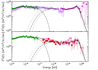
Figure 1: Open squares: Akeno; filled circles: KASCADE; filled diamonds: AGASA; filled squares: HiRes-2; open triangles: Hires-1; open diamonds: Fly’s Eye. Fit of the Galactic (low-energy dot-dash line) and extra-galactic (high-energy dot-dash) to cosmic ray data. Total flux: solid line; dotted lines: upper $75^{\rm th}$ and lower $25^{\rm th}$ percentiles for the prediction of the extra-galactic flux.

III Results and discussion

Figure 1 shows the total spectrum (Galactic + Extra-galactic) compared to the data, assuming continuously emitting sources with density $n=10^{-5}$Mpc^-3 and spectral index $\gamma=2.6$. The solid and dot-dashed lines for the extra-galactic show the median spectrum obtained over $500$ realizations of the source locations. For each realization the locations of the first hundred closest sources (i.e. within $\simeq 140\,$Mpc) were drawn at random, using a uniform probability law per unit volume; for farther sources, the continuous source approximation is valid and it was used numerically. The upper and lower dotted curves show the $75^{\rm th}$ and $25^{\rm th}$ percentiles around this prediction, meaning that only 25% of spectra are respectively higher / respectively lower than indicated by these curves. This uncertainty is related to the location of the closest sources, see below.

Considering the difficulty of comparing different datasets, the fit shown in Fig. 1 appears satisfying. One should also note that this fit uses a minimum number of free parameters ($\gamma$ and $l_{\rm scatt}$ at $10^{17}\,$eV), in order to consider the most economical scenario. As discussed below, there are various ways in which one could extend the present analysis, although this comes at the price of handling a larger number of (unknown) parameters.

In Fig. 1, a straight dashed line was drawn across the region $1.5\cdot 10^{18}\rightarrow 8\cdot 10^{18}\,$eV in which the propagation is neither rectilinear nor diffusive. These limits were found by comparing the diffusive and rectilinear spectra with the no magnetic field spectrum. In this energy range the diffusive path length becomes of the same order as the rectilinear distance at some point during the particle history. The diffusion theorem AB04 suggests that the flux in this intermediate region should follow the no magnetic field spectrum (in which case it would dip $\sim 10\,$% below the dashed line around $3\cdot 10^{18}\,$eV). This theorem rests on the observation that integrating Eq. (1) for a continuous distribution of sources over an infinite volume gives the rectilinear spectrum Eq. (2). However the actual volume is bounded by the past light cone; this is why the diffusive spectrum shuts off exponentially at energies $\gtrsim 10^{18}\,$eV. The rectilinear part shuts off at energies $\lesssim 7\cdot 10^{18}\,$eV as the maximal lookback time that bounds the integral of Eq. (2) decreases sharply. Hence one might expect a small dip in the spectrum around $2-3\cdot 10^{18}\,$eV. Interestingly the data is not inconsistent with such a dip at that location. Monte Carlo simulations of particle propagation are best suited (and should be performed) to probe the spectrum in this region.

The scattering length was assumed to scale as $l_{\rm scatt}\propto E^{2}$, and its value at $10^{18}\,$eV was set here to $17\,$Mpc. This scaling of the scattering length is typical for particles with Larmor radius larger than the coherence scale of the field, in which case $l_{\rm scatt}\simeq l_{\rm c}(r_{\rm L}/l_{\rm c})^{2}$. Since the Larmor radius $r_{\rm L}\simeq 1\,{\rm Mpc}\,(E/10^{18}\,{\rm eV})(B/10^{-9}\,{\rm G})^{-1}$, one may expect this approximation to be valid. In effect, $1\,$Mpc is a strict upper bound to the coherence length of a turbulent inter-galactic magnetic field WB99 ; AB04 , and available numerical simulations indicate much smaller coherence lengths DGST in clusters of galaxies. A value $l_{\rm c}\sim 10\,$kpc could also be expected if the inter-galactic magnetic field is produced by galactic outflows. The above condition for $l_{\rm scatt}$ corresponds to $B\sqrt{l_{\rm c}}\sim 2.5\cdot 10^{-10}\,$G$\cdot$Mpc^1/2 for an all-pervading magnetic field. Hence, for $l_{\rm c}\sim 20\,$kpc, and $B\sim 2\cdot 10^{-9}\,$G (in order to obtain the correct scattering length at $10^{18}\,$eV), one finds $r_{\rm L}\gtrsim l_{\rm c}$ for $E\gtrsim 3\cdot 10^{16}\,$eV.

It is possible that the scaling of $l_{\rm scatt}$ with energy changes in the range $10^{16}\rightarrow 10^{17}\,$eV as $r_{\rm L}$ may become smaller than $l_{\rm c}$. There is no universal scaling for $l_{\rm scatt}$ when $r_{\rm L}<l_{\rm c}$ as the exact relationship then depends on the structure of the magnetic field; for instance, in Kolmogorov turbulence, one finds $l_{\rm scatt}\propto r_{\rm L}$ for $0.1l_{\rm c}\lesssim r_{\rm L}\lesssim l_{\rm c}$ and $l_{\rm scatt}\propto r_{\rm L}^{1/3}$ at lower energies CLP01 . The possible existence of regular components of extra-galactic magnetic fields may also modify $l_{\rm scatt}$. A change in the scaling of $l_{\rm scatt}$ with $E$, if it occurs at $E\gtrsim 10^{16.5}\,$eV, would imply a different value for $B\sqrt{l_{\rm c}}$, with the difference being a factor of order unity to a few. It is exciting to note that, in the present framework, experiments such as KASCADE-Grande KASCADE may allow to constrain the energy dependence of the scattering length (hence the magnetic field structure) by measuring accurately the energy spectrum and composition between the first and second knees.

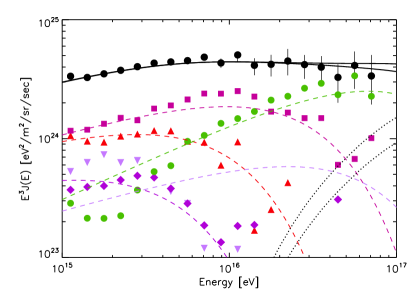
Figure 2: KASCADE (SYBILL) data: solid lines: all-particle spectra (Galactic + extra-galactic); dotted lines: extra-galactic component; dashed lines: Galactic spectra, for p, He, C, Si and Fe, in order of increasing $x-$axis intercept. Filled circles: all-particle; diamonds: p; upward-pointing triangles: He; squares: C; downward pointing triangles: Si; circles: Fe. Error bars on reconstucted chemical composition have been omitted for clarity, but are significant, see  KASCADE .

The predictions (for both normalizations in Fig. 1) for the extra-galactic proton flux are shown and compared to the chemical composition measurement of KASCADE in Fig. 2. These composition measurements remain uncertain, as can be seen by comparing the QGSJet and SYBILL reconstructions in KASCADE ; the proton and helium knee positions seem robust however. The dotted lines represent the median proton signal from the extra-galactic component, whose detection seems within the reach of KASCADE-Grande. One may note that Galactic spectra with exponential suppression beyond the knee agree with the KASCADE data. Nonetheless, if the Galactic spectra are found to extend as powerlaws beyond the knee, the scattering length of extra-galactic protons should be smaller by a factor of order unity (and $B\sqrt{l_{\rm c}}$ correspondingly higher).

The result for $B\sqrt{l_{\rm c}}$ depends weakly on the source density: since the diffusive (low energy) part of the spectrum shuts off as $\exp\left[-r^{2}/4\lambda^{2}\right]$ with $r\sim n^{-1/3}$ the closest source distance, the cut-off energy depends on the ratio $n^{-1/3}/\lambda\propto n^{-1/3}(B\sqrt{l_{\rm c}})$, hence $B\sqrt{l_{\rm c}}$ scales with $n$ according to: $B\sqrt{l_{\rm c}}\sim 2-3\cdot 10^{-10}(n/10^{-5}\,{\rm Mpc}^{-3})^{1/3}\,$G$\cdot$Mpc^1/2.

Cosmic variance related to the distance $d$ to the closest sources is significant for the low energy ($E\lesssim 10^{17}\,$eV) and for the high energy ($E\gtrsim 10^{20}\,$eV) parts of the spectrum, as illustrated by the confidence intervals around the median flux shown in Fig. 1. In these two energy ranges, the effective linear distance to the source is limited to $\lesssim 50\,$Mpc, which is comparable to the expected distance to the closest source. Interestingly, the spectra close to both low and high energy cut-offs are strongly correlated due to the above effect. The distances to within which one should find $N=(1,2,3,4,5)$ sources (with $N$ the Poisson average) are $r\simeq(29,36,41,46,50)\,$Mpc respectively. The diffusive spectrum sums up contributions that scale as $\exp\left[-r_{i}^{2}/4\lambda^{2}\right]$, with $r_{i}$ the distance to the $i^{\rm th}$ closest source. Therefore, close to the cut-off energy, where $r_{1}^{2}/4\lambda^{2}\gg 1$, the total spectrum is dominated on the average by the individual spectrum of the closest or the two closest sources. At higher energies spectra of more remote sources contribute with a weight $\sim\exp\left[-r_{i}^{2}/4\lambda^{2}\right]$. Since what matters most for the comparison to the data is the cut-off energy, one finds that as a first approximation, cosmic variance related to the position of the closest source at distance $r_{1}$ induces an uncertainty of the inferred magnetic field strength $\Delta B/B\sim\Delta d/d\sim{\cal O}(1)$ since, as before, the cut-off energy depends on the ratio $r_{1}/\lambda$.

It is possible that the ultra-high energy cosmic ray sources are intermittent with an activity timescale $T_{\rm source}\ll H_{0}^{-1}$; the previous discussion has assumed steady sources corresponding to $T_{\rm source}\sim H_{0}^{-1}$. If $T_{\rm source}\ll H_{0}^{-1}$, the number density of sources inferred from clustering at high energies ($E\gtrsim 4\cdot 10^{19}\,$eV) underestimates the actual density of potential sources by a factor $T/H_{0}^{-1}$, with $T^{2}\sim T_{\rm source}^{2}+\Delta\tau_{B}^{2}$, and where $\Delta\tau_{B}$ is the typical time spread at $E\sim 4\cdot 10^{19}\,$eV due to magnetic delay. The average time delay reads: $\tau_{B}\sim 1.5\cdot 10^{8}\,{\rm yr}\,(E/10^{19}\,{\rm eV})^{-2}(d/1\,{\rm Gpc})^{2}(B\sqrt{l_{\rm c}}/3\cdot 10^{-10}\,{\rm G}\cdot{\rm Mpc}^{1/2})^{2}$ WM96 ; the ratio $\Delta\tau_{B}/\tau_{B}\lesssim 1$ depends on the structure of the random magnetic field, see WM96 ; Lea97 . Each source then contributes for a fraction $T/H_{0}^{-1}$ of a Hubble time to the diffusive spectrum given in Eq. (1), but there are $H_{0}^{-1}/T$ times more sources: the total flux remains the same than evaluated previously, except that the cut-off energy will correspond to that expected for a source density larger by $H_{0}^{-1}/T$. Hence, following the previous discussion, the present scenario remains valid if the magnetic field strength is higher by a factor $(H_{0}^{-1}/T)^{1/3}$. For instance, for active galactic nuclei sources of ultra-high energy cosmic rays with $T_{\rm source}\sim 10^{8}\,$yr, a fit similar to that shown in Fig. 1 can be obtained for a magnetic field strength $B\sqrt{l_{\rm c}}\sim 10^{-9}\,{\rm G}\cdot{\rm Mpc}^{1/2}$. For the particular case of transient Galactic sources, such as $\gamma-$ray bursts, the situation is different, since the closest sources lie at distance $r_{i}\approx 0$. Therefore the diffusive spectrum $J_{\rm diff}(E)\approx\sum_{i}(c/4\pi)\left[4\pi D(E)t_{i}\right]^{-3/2}q(E)$, since $\lambda^{2}\simeq D(E)t_{i}$ for close by sources, with $t_{i}$ the lookback time to the $i^{\rm th}$ event, and $q(E)$ the injection spectrum per source. Diffusion in extra-magnetic fields thus does not produce a low energy cut-off in this case; the spectrum is rather subject to the fluctuations of the time distribution of past Galactic events.

At high energies, $E\gtrsim 10^{19}\,$eV, particles travel in a quasi-rectilinear fashion, i.e. the deflection angle suffered by crossing a coherence cell of the magnetic field $\delta\theta\sim l_{\rm c}/r_{\rm L}\sim 3\times 10^{-3}(l_{\rm c}/30\,{\rm kpc})(E/10^{19}\,{\rm eV})^{-1}(B/10^{-9}\,{\rm G})$ is much smaller than unity. The total deflection angle summed over the trajectory remains smaller than unity, and this justifies the use of Eq. (2) WM96 : $\theta_{\rm rms}\sim 25^{o}(E/10^{19}\,{\rm eV})^{-1}(d/1\,{\rm Gpc})^{1/2}(B\sqrt{l_{\rm c}}/3\cdot 10^{-10}\,{\rm G}\cdot{\rm Mpc}^{1/2})$. This also implies that charged particle astronomy will be possible at the highest energies. Recent studies have attempted to obtain definite predictions for $\theta_{\rm rms}$ by using MHD simulations of large-scale structure formation with magnetic fields scaled to reproduce existing data in clusters of galaxies DGST ; SME . Their results differ widely, thereby illustrating the difficulty of constraining ab initio the strength of extra-galactic magnetic fields. The present value for $\theta_{\rm rms}$ is comparable to or slightly larger than that of Ref. DGST , and substantially smaller than that of Ref. SME . The magnitude of $\theta_{\rm rms}$ indicates that extra-galactic magnetic fields could be probed through the angular images of ultra-high energy cosmic ray point sources, and this will constitute a strong test of the present scenario.

The proposed scattering length cannot result from scattering on magnetic fields associated with galaxies or groups and clusters of galaxies, since the collision mean free path with either of these objects is too large, being $\sim{\cal O}(1\,{\rm Gpc})$. The inferred magnetic field might in principle be concentrated around the source (on distance scale $L$) and negligible everywhere else. Since the spectrum would cut off below an energy such that $2\lambda\approx 2\left[cH_{0}^{-1}l_{\rm scatt}\right]^{1/2}\lesssim L$, this requires $B\gtrsim 1\,\mu{\rm G}\,(l_{\rm c}/10\,{\rm kpc})^{-1/2}(L/100\,{\rm kpc})^{-1}$ (for a cut-off at $10^{17}\,$eV). This possibility cannot be excluded but it gives a non-trivial constraint on the source environment. Searches for counterparts at the highest energies would help test this possibility: for instance, magnetic fields such as above are found in clusters of galaxies but there is no report of clusters in the arrival directions of the highest energy events. If this magnetic field is intrinsic to the source, or if the cut-off at $\lesssim 10^{18}\,$eV is due to injection physics in the source BGG2 , then, under the present assumptions, the present work still gives a stringent upper bound on all-pervading magnetic fields. To remain conservative, one may require that the cut-off should not occur above $\sim 10^{18}\,$eV, in which case one finds $B\sqrt{l_{\rm c}}\lesssim 10^{-9}\,$G$\cdot$Mpc^1/2. This limit is still an order of magnitude below existing Faraday bounds.

The magnetic field in question thus appears inter-galactic in nature, in which case it is likely to be inhomogeneously distributed on small scales. Further studies are then required to relate the average $B\sqrt{l_{\rm c}}$ with the actual structure and distribution of these magnetic fields. One needs to account for the possible existence of a regular magnetic field component aligned with filaments and walls, which would inhibit perpendicular transport, and consider the respective filling fractions and amplitudes of the turbulent and regular components. It would be certainly worthwhile to extend the simulations of particle propagation made in realistic magnetic fields DGST ; SME to the energies of interest.

Finally there are various ways in which the present study could be extended. One should notably consider the possible energy dependences of the scattering length (including the above effects of inhomogeneous and regular magnetic fields), the role of intermittent sources, the possible cosmological evolution of the magnetic field and of the source density, and, as mentioned above, the possibly inhomogeneous structure of the magnetic field on a scale comparable to the closest ultra-high energy cosmic ray sources.

*

Appendix A Diffusion over cosmological scales

The diffusion of particles in an expanding background space-time can be seen as a standard diffusion process on a fixed background in conformal coordinates $(\eta,{\mathbf{r}})$, with $\eta$ the conformal time defined by $a(\eta){\rm d}\eta={\rm d}t$ and ${\mathbf{r}}$ the comoving coordinates in a Friedman-Lemaître-Robertson-Walker metric; $a$ denotes the scale factor and $t$ cosmic time. One can indeed approximate the diffusing process as a random walk against scattering centers of constant comoving coordinates.

Particles also experience dilution due to expansion, expansion energy losses and energy losses due to pair and pion production on diffuse backgrounds. At redshift $z=0$, these photo-interaction losses are negligible with respect to expansion losses for energies $E\lesssim 2\cdot 10^{18}\,$eV, but become increasingly more important at higher redshift due to the increased cosmic microwave background temperature and density BGG1 . Nonetheless the main energy loss in the course of the history of a particle with present energy $E_{0}\lesssim 10^{18}\,$eV is due to expansion. One reason is that the majority of the sources that contribute to the diffuse flux at energy $E_{0}$ are located at moderate redshifts as a result of the nonlinear time-redshift relation: redshift $z=2$, for instance, corresponds to a lookback time of $76$% of the age of the Universe cosmology . More importantly, pion and pair production losses at high redshift become catastrophic, so that the time interval during which the losses are dominated by photo-interactions is much smaller than a Hubble time. Finally, the contribution to the diffuse flux at energy $E_{0}$ of particles injected with energy $E_{\rm g}$ scales, in a first approximation, as $q(E_{\rm g}){\rm d}E_{\rm g}/{\rm d}E$, with $q(E_{\rm g})$ the injection spectrum and ${\rm d}E_{\rm g}/{\rm d}E$ acounts for the dilation of the energy interval. The function $E_{\rm g}(\eta,E)$ defines the energy of the particle at time $\eta$, assuming it has energy $E$ at time $t_{0}$. This function and its derivative ${\rm d}E_{\rm g}/{\rm d}E$ can be reconstructed by integrating the energy losses BGG1 . Assuming ${\rm d}E_{\rm g}/{\rm d}E\approx E_{\rm g}/E$, which is exact for expansion losses, one sees that the contribution of particles injected at remote lookback times (hence with high $E_{\rm g}$) is negligible with respect to that of particles injected recently with $E_{\rm g}\approx E$ since $q(E_{\rm g})\propto E_{\rm g}^{-\gamma}$ and $\gamma\sim 2.6$ here. The numerical difference between a diffuse flux computed using only expansion losses and that computed with all energy losses included is indeed less than $5$% at $E\ll 10^{18}\,$eV, and increases to $20$% at $E\sim 10^{18}\,$eV. Consequently, it is assumed in this discussion that particles with present $E_{0}\lesssim 10^{18}\,$eV have been subject to expansion losses only throughout their history.

Energy losses due to expansion are expressed as: ${\rm d}E/{\rm d}\eta=-{\cal H}E$, with ${\cal H}\equiv(1/a){\rm d}a/{\rm d}\eta$ the expansion rate in conformal time. The phase space density of particles $N(\eta,E,{\mathbf{r}})$ at coordinates ${\mathbf{r}}$, time $\eta$ and energy $E$, which is related to the distribution function by $N(\eta,E,{\mathbf{r}})=(4\pi p^{2}/c)f(\eta,{\mathbf{p}},{\mathbf{r}})$, with $pc=E$, is solution to the diffusion equation:

$${\partial\over\partial\eta}\left(a^{3}N\right)-\nabla D\nabla\left(a^{3}N\right)-{\cal H}{\partial\over\partial E}\left(Ea^{3}N\right)\,=\,a^{3}\tilde{Q}\left(\eta,E,{\mathbf{r}}\right),$$ (3)

where $\tilde{Q}$ gives the (physical) number density of particles injected per unit energy and conformal time intervals. The $a^{3}$ prefactor of $N$ takes into account the effect of dilution of particle density through expansion. The fact that expansion losses are separable in terms of the two variables $E$ and $\eta$ allows to find an exact solution to this diffusion equation, using standard Green functions methods; see S59 for the same problem with time independent losses in a non-expanding background. Explicitly, through the change of variables $(\eta,E)\rightarrow(u,v)$, with $u=\log(aE)$ and $v=\log(a/E)$, one can derive the Green function (for the equation for $N$) as:

$$G\left(\eta_{0},E_{0},{\mathbf{r}}_{0};\eta_{e},E_{e},{\mathbf{r}}_{e}\right) \,=\, \left({a_{e}\over a_{0}}\right)^{2}{\exp\left[-{|{\mathbf{r}_{0}-\mathbf{r}_{e}}|^{2}\over 4\lambda^{2}}\right]\over\left(4\pi\lambda^{2}\right)^{3/2}}$$ (4)

$$\times\delta\left(E_{e}-{a_{0}E_{0}\over a_{e}}\right),$$

with the shorthand notations: $a_{0}\equiv a(\eta_{0})$ and $a_{e}\equiv a(\eta_{e})$. The path length $\lambda$ is defined by:

$$\lambda^{2}\,=\,\int_{\eta_{e}}^{\eta_{0}}{\rm d}\eta\,D\left[{a_{e}E_{e}\over a(\eta)}\right],$$ (5)

where $D(E)$ is the diffusion coefficient; if this latter depends explicitly on time, for instance if the magnetic field strength evolves with redshift, the solution remains valid.

References

- (1) R. U. Abbasi et al. (HiRes collaboration), PRL 92 (2004) 151101.
- (2) K.-H. Kampert et al. (KASCADE collaboration), arXiv:astro-ph/0405608.
- (3) V. Berezinsky, A. Gazizov, S. Grigorieva, arXiv:hep-ph/0204357; arXiv:astro-ph/0210095
- (4) see for instance T. Wibig, A. Wolfendale, arXiv:astro-ph/0410624.
- (5) V. S. Berezinsky, S. I. Grigorieva, B. I. Hnatyk, Astropart.Phys.21 (2004) 617.
- (6) L. M. Widrow, Rev.Mod.Phys.74 (2003) 775 and references therein.
- (7) P. Blasi, D. de Marco, Astropart.Phys. 20 (2004) 559; H. Yoshiguchi, S. Nagataki, S. Tsubaki, K. Sato, Astrophys.J. 586 (2003) 1211; M. Kachelriess, D. Semikoz, arXiv:astro-ph/0405258.
- (8) Similar magnetic horizons effects have been noted in C. Isola, M. Lemoine, G. Sigl G., 2001, PRD 65 (2002) 023004; T. Stanev, arXiv:astro-ph/0303123 (2003); O. Deligny, A. Letessier-Selvon, E. Parizot, Astropart.Phys.21 (2004) 609; T. Wibig, A. Wolfendale, arXiv:astro-ph/0406511 (2004).
- (9) V. Springel, L. Hernquist, Month. Not. Roy. Astron. Soc. 339 (2003) 312.
- (10) L. E. Strigari, J. F. Beacom, T. P. Walker, P. Zhang, arXiv:astro-ph/0502150 (2005).
- (11) M. Nagano et al. (Akeno collaboration), J.Phys.G18 (1992) 423.
- (12) M. Takeda et al. (AGASA collaboration), PRL 81 (1998) 1163.
- (13) D. J. Bird et al. (Fly’s Eye collaboration), Astrophys.J.424 (1994) 491.
- (14) R. Aloisio, V. S. Berezinsky, arXiv:astro-ph/0403095.
- (15) E. Waxman, J. N. Bahcall, PRD 59 (1999) 023002.
- (16) K. Dolag, D. Grasso, V. Springel, I. Tkachev, JETP Lett.79 (2004) 583 [Pisma Zh.Eksp.Teor.Fiz.79 (2004) 719]; arXiv:astro-ph/0410419.
- (17) F. Casse, M. Lemoine, G. Pelletier, PRD 65 (2002) 023002; J. Candia, E. Roulet, JCAP 0410 (2004) 007.
- (18) E. Waxman, J. Miralda-Escudé, Astrophys. J. 472 (1996) L89.
- (19) M. Lemoine, G. Sigl, A. Olinto, D. Schramm, Astrophys. J. 486 (1997) L115; G. Sigl, M. Lemoine, Astropart. Phys. 9 (1998) 65.
- (20) G. Sigl, F. Miniati, T. A. Ensslin, PRD 68 (2003) 043002; arXiv:astro-ph/0309695; PRD 70 (2004) 043007.
- (21) It is assumed that , , km/s/Mpc.
- (22) S. I. Syrovastkii, Sov. Astron. 3 (1959) 22 [Astron. Zh. 36 (1959) 17].