ON THE METHOD OF ESTIMATING EMISSION ALTITUDE FROM RELATIVISTIC PHASE SHIFT IN PULSARS

Abstract

The radiation by relativistic plasma particles is beamed in the direction of field line tangents in the corotating frame, but in an inertial frame it is aberrated toward the direction of rotation. We have revised the relation of aberration phase shift by taking into account of the colatitude of emission spot and the plasma rotation velocity. In the limit of small angle approximation, aberration phase shift becomes independent of the inclination angle $\alpha$ and the sight line impact angle $\beta.$ However, at larger altitudes or larger rotation phases, the shift does depend on $\alpha$ and $\beta.$ We have given an expression for the phase shift in the intensity profile by taking into account of aberration, retardation and polar cap currents. We have re-estimated the emission heights of the six classical pulsars, and analyzed the profile of a millisecond pulsar PSR J0437-4715 at 1440 MHz by fitting the Gaussians to pulse components. By this procedure we have been able to identify 11 emission components of PSR J0437-4715. We propose that they form a emission beam with 5 nested cones centered on the core. Using the phase location of component peaks, we have estimated the relativistic phase shift and the emission height of conal components. We find some of the components are emitted from the altitudes as high as 23 percent of light cylinder radius.

1 INTRODUCTION

The profile morphology and polarization of pulsars has been widely attempted to interpret in terms of emission in dipolar magnetic field lines (e.g., Radhakrishan & Cooke 1969; Sturrock 1971; Ruderman & Sutherland 1975; Lyne & Manchester 1988; Blaskiewicz et al. 1991; Rankin 1983a&b, 1990, 1993; Hibschman & Arons 2001). Most of the radio emission models assume (1) radiation is emitted by the relativistic secondary pair plasma, (2) beamed radio waves are emitted in the direction of field line tangents, and (3) emitted radiation is polarized in the plane of dipolar field lines or in the perpendicular directions.

From the theoretical point of view, it is highly preferable to know the precise altitude of radio emission region in the pulsar magnetosphere. By knowing the emission altitude, one can infer the probable plasma density, rotation velocity, magnetic field strength, field line curvature radii etc, which prevail in the radio emission region. For estimating the radio emission altitudes two kinds of methods have been proposed: (1) Purely geometric method, which assumes the pulse edge is emitted from last open field lines (e.g., Cordes 1978; Gil & Kijak 1993; Kijak & Gil 2003), (2) Relativistic phase shift method, which assumes the asymmetry in the conal components phase location, relative to core, is due to the aberration-retardation phase shift (e.g., Gangadhara & Gupta 2001, hereafter GG01). By estimating the phase lag of polarization angle inflection point with respect to the centroid of the intensity pulse, Blaskiewicz et al. (1991) have estimated the emission heights. The results of purely geometric method are found to be in rough agreement with those of Blaskiewicz et al. (1991). However, compared to geometric method, the emission heights estimated from relativistic phase shift are found to be notably larger, particularly in the case of nearly aligned rotators (Gupta & Gangadhara 2003, hereafter GG03). Dyks, Rudak and Harding (2004, hereafter DRH04) by revising the relation for aberration phase shift given by GG01, have re-estimated the emission heights. In the small angle approximation, they have found that the revision furnishes a method for estimating radio emission altitudes, which is free of polarization measurements and does not depend on $\alpha$ the magnetic axis inclination angle and $\beta$ the sight line impact angle. By assuming the beamed radio waves are emitted in the direction of field line tangents, Gangadhara (2004, hereafter G04) has solved the viewing geometry in an inclined and rotating dipole magnetic field.

In §2, we derive the angle between the corotation velocity of particles/plasma bunches and dipolar magnetic field. Using the magnetic colatitude and azimuth of the emission spot in an inclined and rotating dipole, we have derived the phase shift due to aberration, retardation and polar cap current in §3, and the emission radius in §4. In §5, we compare the shifts due to various process. As an application of our model, in §6, we have re-estimated the emission heights of six classical pulsars. Further, by considering a mean profile of a millisecond pulsar PSR J0437-4715, we have estimated the relativistic phase shift in conal components and their emission heights.

2 ANGLE BETWEEN PLASMA ROTATION VELOCITY AND DIPOLAR MAGNETIC FIELD

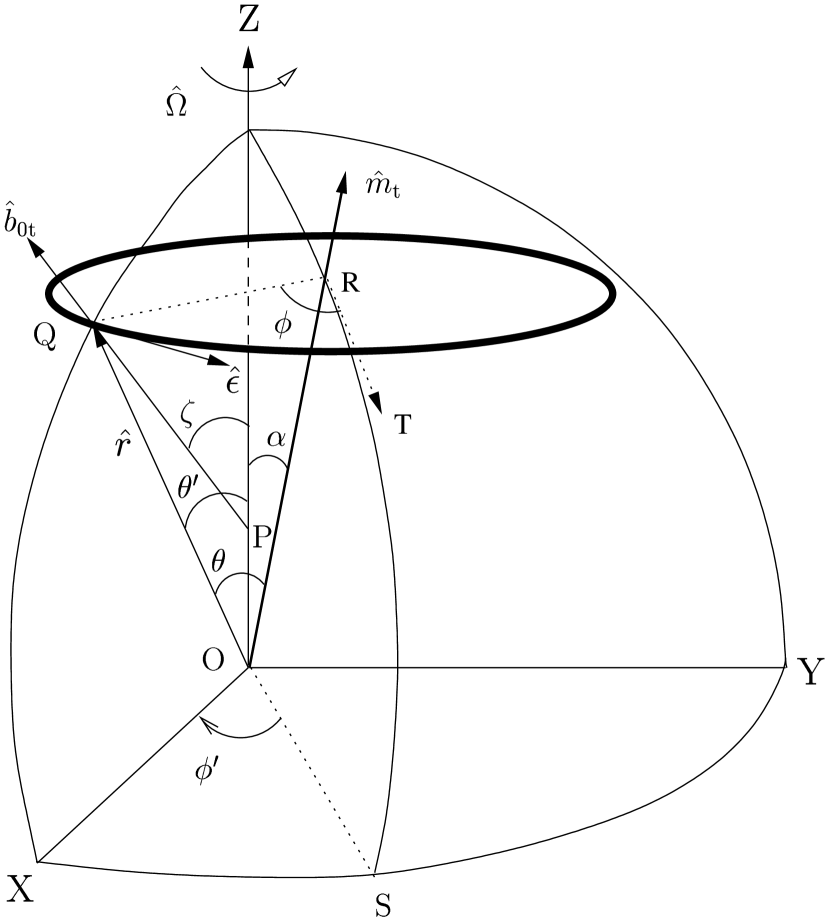
Figure 1: Viewing geometry of emission beam. The heavy line ellipse represents the cone of emission centered on the magnetic axis ${\hat{m}}_{\rm t}$. The arcs ZQX, ZRS, ZY and XSY represent the great circles centered at O (star center). The magnetic colatitude $\phi$ and the phase angle $\phi^{\prime}$ of the emission spot are measured from the meridional $(\Omega,~{}{\hat{m}}_{\rm t})$ plane. They have the signs in such a way that $\phi^{\prime}$ is positive while $\phi$ is negative on the trailing side, and the vice versa on leading side.

Consider an inclined and rotating magnetic dipole ($\hat{m}_{\rm t}$) with the rotation axis $\hat{\Omega},$ as shown in Figure 1. The angles $\alpha$ and $\phi^{\prime}$ are the magnetic axis inclination angle and the rotation phase, respectively. Assume that the relativistic secondary plasma flows along the dipolar field lines, and emit the beamed radiation in the direction of field line tangents $(\hat{b}_{\rm 0t}).$ In a non-rotating case, to receive such an emission the sight line $(\hat{n})$ must line up with $\hat{b}_{\rm 0t}.$ Let Q be the emission point on a field line at which $\hat{n}=(\sin\zeta,0,\cos\zeta)$ is parallel $\hat{b}_{\rm 0t},$ where $\zeta=\alpha+\beta$ and $\beta$ is the sight line impact angle relative to $\hat{m}_{\rm t}.$ The angles $\angle{\rm QOR}=\theta$ and $\angle{\rm QRT}=\phi$ are the magnetic colatitude and azimuth of Q relative to $\hat{m}_{\rm t}$, respectively. While $\angle{\rm QOZ}=\theta^{\prime}$ and $\angle{\rm XOS}=\phi^{\prime}$ are the colatitude and azimuth of Q relative to rotation axis, respectively.

The position vector of Q is given by ${\bf r}_{\rm ct}$ (see eq. 2 in G04). For brevity we shall drop the suffix, and take ${\bf r}={\bf r}_{\rm ct}.$ The angle between $\bf r$ and $\hat{\Omega}$ is given by

$$\cos\theta^{\prime}=\hat{\Omega}.\hat{r}=\cos\alpha\,\cos\theta-\sin\alpha\,\sin\theta\,\cos\phi~{},$$ (1)

where the unit vector $\hat{r}={\bf r}/|{\bf r}|,$ and the expressions for $\theta$ and $\phi$ as functions of $\phi^{\prime},$ $\alpha$ and $\beta$ are given in G04.

For the field line which lies in the meridional plane, defined by $\hat{\Omega}$ and $\hat{m}_{\rm t},$ we have $\theta^{\prime}_{\rm min}=\alpha+\theta_{\rm min}.$ The magnetic colatitude $\theta_{\rm min}$ of Q can be obtained by setting $\phi^{\prime}=0$ in equation (9) of G04:

$$\theta_{\rm min} = \frac{1}{2}\arccos\!\!\left(\frac{\cos(2\beta)+{\sqrt{2}}\cos\beta{\sqrt{17+\cos(2\beta)}}-1}{6}\right)$$ (2)

$$\approx \frac{2}{3}\beta+O(\beta)^{3}\quad\quad\hbox{for}\quad\beta\ll 1.$$

This is the minimum value, which $\theta$ takes at $\phi^{\prime}=0.$

The rotation velocity of the plasma particle (bunch) at Q is given by

$${\bf v}_{\rm rot}={\bf\Omega}\times{\bf r}=\Omega r\sin\theta^{\prime}\,\hat{\epsilon}\,,$$ (3)

where $\bf\Omega$ is the pulsar angular velocity, and the unit vector $\hat{\epsilon}$ represents the direction of rotation. Consider a Cartesian coordinate system - XYZ, with Z-axis parallel to the rotation axis and X-axis lies in the fiducial plane defined by $\hat{n}$ and $\hat{\Omega}.$ Let $\Theta$ be the angle between the field line tangent $\hat{b}_{\rm 0t}$ and $\hat{\epsilon},$ then we have

$$\hat{\epsilon}=\cos\Theta\,\hat{\epsilon}_{\parallel}+\sin\Theta\,\hat{\epsilon}_{\perp}\,,$$ (4)

where the unit vectors $\hat{\epsilon}_{\parallel}$ and $\hat{\epsilon}_{\perp}$ are parallel and perpendicular to $\hat{b}_{\rm 0t}.$ Therefore, the angle $\Theta$ is given by

$$\cos\Theta=\hat{\epsilon}.{\hat{b}_{\rm 0t}}=\frac{a_{1}}{{\sqrt{(1+4\,a^{2}_{2})a_{3}}}}~{},$$ (5)

where

$$a_{1}=\sin\alpha\,\sin\phi,\quad a_{2}=\cot\theta,$$

$$a_{3}=\frac{{\cos^{2}\alpha}\,{\cos^{2}\phi}+a^{2}_{2}\,{\sin^{2}\alpha}+{a_{2}}\,\cos\phi\,\sin(2\,\alpha)+{\sin^{2}\phi}}{1+a^{2}_{2}}.$$

We have plotted $\Theta$ as a function of rotation phase $\phi^{\prime}$ for different $\alpha$ in Figure 2. It shows $\Theta=90^{\circ}$ for the field lines which lie in the meridional plane ($\phi^{\prime}=0$) but for other field lines it is $<90^{\circ}$ on leading side and $>90^{\circ}$ in the trailing side. But for an aligned rotator $(\alpha=0^{\circ}),$ it is $90^{\circ}$ for all the field lines.

3 PHASE SHIFT OF RADIATION EMITTED BY A PARTICLE (BUNCH)

Since the pulsar spin rate is quite high, the rotation effects such as the aberration and retardation play an important role in the morphology of pulse profiles. For an observer in an inertial frame, the radiation beam gets phase shifted due to the corotation of plasma particles and the difference in emission radii.

Since the radiation by a relativistic particle is beamed in the direction of velocity, to receive it sight line must align with the particle velocity within the angle $1/\gamma,$ where $\gamma$ is the Lorentz factor. The particle velocity is given by

$${\bf v}=\kappa c\,{\hat{b}}_{\rm 0t}+{\bf v}_{\rm rot},$$ (6)

where $c$ is the speed of light. By substituting for ${\bf v}_{\rm rot}$ from equation (3) into equation (6) we obtain

$${\bf v}=(\kappa c+\Omega r\sin\theta^{\prime}\cos\Theta)\,{\hat{b}}_{\rm 0t}+\Omega r\sin\theta^{\prime}\sin\Theta\,\hat{\epsilon}_{\perp}\,.$$ (7)

By assuming $|{\bf v}|\sim c,$ from equation (7) we obtain the parameter

$$\kappa=\sqrt{1-\left(\frac{\Omega r}{c}\right)^{2}\sin^{2}\theta^{\prime}\sin^{2}\Theta}-\frac{\Omega r}{c}\sin\theta^{\prime}\cos\Theta\,.$$ (8)

In Figure 3, we have plotted $\kappa$ as a function of $r$ for different $\alpha.$ It shows $\kappa\sim 1$ for $r/r_{{}_{\rm LC}}\ll 1,$ but at large $r$ it decreases from unity due to increase in rotation velocity, where $r_{{}_{\rm LC}}$ is the light cylinder radius. Machabeli & Rogava (1994), by considering the motion of a bead inside a rotating linear tube, have deduced a similar behavior in the velocity components of bead.

Using equation (3) we can solve equation (4) for $\hat{\epsilon}_{\perp},$ and obtain

$$\hat{\epsilon}_{\perp}=\frac{\hat{\Omega}\times\hat{r}}{\sin\theta^{\prime}\sin\Theta}-\cot\Theta\,\hat{b}_{\rm 0t}~{}.$$ (9)

Let $\psi$ be the angle between the rotation axis and $\bf v,$ then we have

$$\cos\psi=\hat{\Omega}.{\hat{v}} = \cos\zeta\left(\sqrt{1-\left(\frac{\Omega r}{c}\right)^{2}\sin^{2}\theta^{\prime}\sin^{2}\Theta}-\frac{\Omega r}{c}\sin\theta^{\prime}\cos\Theta\right)~{}$$ (10)

$$= \kappa\,\cos\zeta~{},$$

where ${\hat{v}}={\bf v}/|{\bf v}|.$ For $r/r_{{}_{\rm LC}}\ll 1,$ it reduces to $\psi\sim\zeta.$

3.1 Aberration Angle

If $\eta$ is the aberration angle, then we have

$$\cos\eta = {\hat{b}}_{\rm 0t}\cdot{\hat{v}}=\frac{\kappa c+\Omega r\sin\theta^{\prime}\cos\Theta}{|\bf v|}~{},$$ (11)

$$\sin\eta = \hat{\epsilon}_{\perp}\cdot{\hat{v}}=\frac{\Omega\,r}{|\bf v|}\sin\theta^{\prime}\sin\Theta~{}.$$ (12)

Therefore, from equations (11) and (12), we obtain

$$\tan\eta=\frac{\Omega r}{c}{\sin\theta^{\prime}\sin\Theta\over\sqrt{1-(\Omega r/c)^{2}\sin^{2}\theta^{\prime}\sin^{2}\Theta}}.$$ (13)

Hence the radiation beam, which is centered on the direction of $\bf v,$ gets tilted (aberrated) with respect to ${\hat{b}}_{\rm 0t}$ due to rotation.

For $\Omega r/c\ll 1$, it can be approximated as

$$\tan\eta\approx\frac{\Omega r}{c}\sin\theta^{\prime}\sin\Theta~{}.$$ (14)

3.2 Aberration Phase Shift

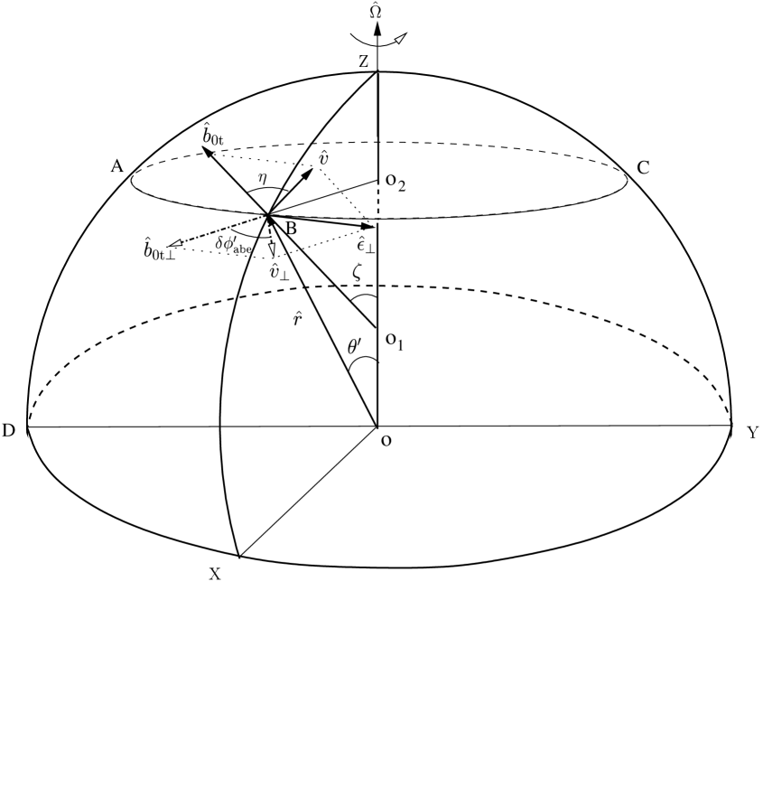
Figure 4: Celestial sphere describing the aberration phase shift of pulsar radio emission, where $\eta$ is the aberration angle, and $\delta\phi^{\prime}_{\rm abe}$ is the corresponding phase shift.

Consider Figure 4 in which ZAD, ZBX, ZCY and DXY are the great circles centered on the neutron star. The small circle ABC is parallel to the equatorial great circle DXY. The unit vector $\hat{b}_{\rm 0t}$ represents a field line tangent, which makes the angle $\zeta$ with respect to the rotation axis ZO. The velocity unit vector $\hat{v}$ is inclined by the angles $\eta$ and $\psi$ with respect to $\hat{b}_{\rm 0t}$ and ZO, respectively. We resolve the vectors $\hat{b}_{\rm 0t}$ and $\hat{v}$ into the components parallel and perpendicular to the rotation axis:

$$\hat{b}_{\rm 0t}=\sin\zeta~{}\hat{b}_{\rm 0t\perp}+\cos\zeta~{}\hat{\Omega}~{},$$ (15)

$$\hat{v}=\sin\psi~{}\hat{v}_{\rm\perp}+\cos\psi~{}\hat{\Omega}~{},$$ (16)

where the unit vectors $\hat{b}_{\rm 0t\perp}$ and $\hat{v}_{\rm\perp}$ lie in the plane of small circle ABC. Next, by solving for $\hat{b}_{\rm 0t\perp}$ and $\hat{v}_{\rm\perp}$, we obtain

$$\hat{b}_{\rm 0t\perp}={1\over\sin\zeta}(\hat{b}_{\rm 0t}-\cos\zeta~{}\hat{\Omega})~{},$$ (17)

$$\hat{v}_{\rm\perp}={1\over\sin\psi}(\hat{v}-\cos\psi~{}\hat{\Omega}~{}).$$ (18)

By taking scalar product with $\hat{b}_{\rm 0t\perp}$ on both sides of equation (18), we obtain

$$\cos(\delta\phi^{\prime}_{\rm abe})=\hat{v}_{\rm\perp}\cdot\hat{b}_{\rm 0t\perp}={1\over\sin\psi}(\hat{v}\cdot\hat{b}_{\rm 0t\perp}-\cos\psi~{}\hat{\Omega}\cdot\hat{b}_{\rm 0t\perp}~{}).$$ (19)

Since $\hat{\Omega}$ and $\hat{b}_{\rm 0t\perp}$ are orthogonal, we have

$$\cos(\delta\phi^{\prime}_{\rm abe})={1\over\sin\psi}(\hat{v}\cdot\hat{b}_{\rm 0t\perp}).$$ (20)

Using $\hat{b}_{\rm 0t\perp}$ from equation (17) we obtain

$$\cos(\delta\phi^{\prime}_{\rm abe})={1\over\sin\psi}{(\hat{v}\cdot\hat{b}_{\rm 0t}-\cos\zeta~{}\hat{v}\cdot\hat{\Omega})\over\sin\zeta}.$$ (21)

By substituting for $\hat{v}\cdot\hat{b}_{\rm 0t}$ and $\hat{v}\cdot\hat{\Omega}$ from equations (11) and (10), we obtain

$$\cos(\delta\phi^{\prime}_{\rm abe})={1\over\sin\psi}{(\cos\eta-\cos\zeta~{}\cos\psi)\over\sin\zeta}.$$ (22)

Substituting for $\eta$ again from equation (11), we obtain

$$\cos(\delta\phi^{\prime}_{\rm abe})={1\over\sin\zeta\sin\psi}\left(\kappa+{\Omega r\over c}\sin\theta^{\prime}\cos\Theta-\cos\zeta\cos\psi\right).$$ (23)

By substituting for $\kappa$ from equation (10), we obtain

$$\cos(\delta\phi^{\prime}_{\rm abe})={1\over\sin\zeta\sin\psi}\left(\frac{\cos\psi}{\cos\zeta}+\frac{\Omega r}{c}\sin\theta^{\prime}\cos\Theta-\cos\zeta\cos\psi\right).$$ (24)

It can be further reduced to

$$\cos(\delta\phi^{\prime}_{\rm abe})=\tan\zeta\cot\psi+\frac{\Omega r}{c}\frac{\sin\theta^{\prime}\cos\Theta}{\sin\zeta\sin\psi}.$$ (25)

Next, by taking a scalar product with $\hat{\Omega}\times\hat{b}_{\rm 0t\perp}$ on both sides of equation (18), we obtain

$$\sin(\delta\phi^{\prime}_{\rm abe})=(\hat{\Omega}\times\hat{b}_{\rm 0t\perp})\cdot\hat{v}_{\rm\perp}={1\over\sin\zeta\sin\psi}(\hat{\Omega}\times\hat{b}_{\rm 0t})\cdot\hat{v}~{}~{}.$$ (26)

By substituting for $\hat{v}$ from equation (7), we obtain

$$\sin(\delta\phi^{\prime}_{\rm abe})={\Omega r\over c}{\sin\theta^{\prime}\sin\Theta\over\sin\zeta\sin\psi}(\hat{\Omega}\times\hat{b}_{\rm 0t})\cdot\hat{\epsilon}_{\perp}~{}~{}.$$ (27)

Using $\hat{\epsilon}_{\perp}$ from equation (9), it can be further reduced to

$$\sin(\delta\phi^{\prime}_{\rm abe})={\Omega r\over c}{A\over\sin\psi}~{},$$ (28)

where

$$A = (\hat{\Omega}\times\hat{b}_{\rm 0t})\cdot(\hat{\Omega}\times\hat{r})/\sin\zeta$$

$$= \cos\phi^{\prime}(\cos\theta\sin\alpha+\cos\alpha\cos\phi\sin\theta)-\sin\phi^{\prime}\sin\phi\sin\theta.$$

Thus, we obtain from equations (25) and (28):

$$\tan(\delta\phi^{\prime}_{\rm abe})={(\Omega r/c)\sin\zeta\,A\over\sin\zeta\tan\zeta\cos\psi+(\Omega r/c)\sin\theta^{\prime}\cos\Theta}~{}.$$ (29)

The aberration phase shift $\delta\phi^{\prime}_{\rm abe}$ is plotted as a function of $\beta$ in Figure 5 for different $\alpha$ in the two cases: (1) $\phi^{\prime}=0^{\circ}$ and $r/r_{{}_{\rm LC}}=0.1,$ and (2) $\phi^{\prime}=60^{\circ}$ and $r/r_{{}_{\rm LC}}=0.1.$ The Figure 5a shows for $\alpha\sim 90^{\circ},$ $\delta\phi^{\prime}_{\rm abe}\approx r/r_{{}_{\rm LC}},$ which is nearly independent of $\beta.$ But, for other values of $\alpha,$ it does depend on $\beta:$ larger for $\beta<0$ and smaller for $\beta>0.$ Since $\theta^{\prime}$ decreases with $|\phi^{\prime}|,$ and $\Theta<90^{\circ}$ on leading side and $>90^{\circ}$ on trailing side, $\delta\phi^{\prime}_{\rm abe}$ is smaller in Figure 5b compared to its corresponding values in Figure 5a. Further, we note that $\delta\phi^{\prime}_{\rm abe}$ has negative gradient with respect to $|\phi^{\prime}|$ for both the signs of $\beta.$ In Figure 6a, $\delta\phi^{\prime}_{\rm abe}$ is plotted as a function of $\phi^{\prime}$ for different $\alpha$ and fixed $\beta=4^{\circ}.$ It is highest at large $\alpha$ and small $|\phi^{\prime}|.$

For $r/r_{\rm LC}\ll 1,$ we can series expand $\delta\phi^{\prime}_{\rm abe}$ and obtain

$$\delta\phi^{\prime}_{\rm abe}=b_{1}\,r_{\rm n}+b_{2}\,r_{\rm n}^{2}+O(r_{\rm n})^{3}~{},$$ (30)

where $r_{\rm n}=r/r_{\rm LC},$

$$b_{1} = {A\over\sin\zeta}~{},$$

$$b_{2} = -\cot^{2}\zeta\cos\Theta\sin\theta^{\prime}\,b_{1}~{}.$$

3.3 Retardation phase shift

Let $\theta_{\rm e},$ $\phi_{\rm e}$ and $\hat{r}_{\rm e}$ be the magnetic colatitude, azimuth and the position vector of the emission spot at the emission time. In the expressions for $\theta$ and $\phi$ (see eqs. 9 and 11 in G04) we replace $\phi^{\prime}$ by $\phi^{\prime}+\delta\phi^{\prime}_{\rm abe}$ to obtain $\theta_{\rm e}$ and $\phi_{\rm e}.$ Then using the values of $\theta_{\rm e}$ and $\phi_{\rm e}$ we find the unit vector $\hat{r}_{\rm e}$ (see eq. 2 in G04). For brevity, we shall drop the suffix on $\hat{r}.$ Note that $\phi^{\prime}>0$ on the trailing side (Fig. 1). Consider the emission radii $r_{1}$ and $r_{2}$ such that $r_{1}<r_{2}.$ The time taken by the signal emitted at the radius ${\bf r}_{1}$ is given by

$$t_{1}={1\over c}(d-{\bf r}_{1}\cdot\hat{n}),$$ (31)

where $d$ is the distance to the pulsar, and $\hat{n}=(\sin\zeta,\,0,\,\cos\zeta)$ is the unit vector pointing toward the observer. For another radius ${\bf r}_{2},$ the propagation time is given by

$$t_{2}={1\over c}(d-{\bf r}_{2}\cdot\hat{n}),$$ (32)

The radiation emitted at the lower radius ${\bf r}_{1}$ takes more time to reach the observer than the one emitted at ${\bf r}_{2}.$ The time delay between the two signals is given by

$$\delta t=t_{1}-t_{2}={1\over c}({\bf r}_{2}\cdot\hat{n}-{\bf r}_{1}\cdot\hat{n}).$$ (33)

By considering the neutron star center (${\bf r}_{1}=0$) as the reference and ${\bf r}_{2}={\bf r},$ we obtain

$$\delta t={r\over c}({\hat{r}}\cdot\hat{n}).$$ (34)

Let $\sigma$ be the angle between $\hat{r}$ and $\hat{n}$, then we have

$$\cos\sigma={\hat{r}}\cdot\hat{n} = \cos\zeta(\cos\alpha\cos\theta_{\rm e}-\cos\phi_{\rm e}\sin\alpha\sin\theta_{\rm e})-\sin\zeta[\sin\phi^{\prime}\sin\phi_{\rm e}\sin\theta_{\rm e}-$$ (35)

$$\cos\phi^{\prime}(\cos\theta_{\rm e}\sin\alpha+\cos\alpha\cos\phi_{\rm e}\sin\theta_{\rm e})].$$

The time delay $\delta t$ of components emitted at lower heights, shifts them to later phases of the profile by (e.g., Phillips 1992)

$$\delta\phi^{\prime}_{\rm ret}=\Omega\delta t={\Omega r\over c}\cos\sigma~{}.$$ (36)

In Figure 6b, $\delta\phi^{\prime}_{\rm ret}$ is plotted as a function of $\phi^{\prime}$ for different $\alpha$ and fixed $\beta=4^{\circ}$. At small $\alpha,$ it is nearly constant and larger. But at larger $\alpha$ it falls with respect to $|\phi^{\prime}|,$ as $\hat{r}$ inclines more from $\hat{n}.$

For $r_{\rm n}\ll 1,$ we can find the series expansion:

$$\delta\phi^{\prime}_{\rm ret}=c_{1}\,r_{\rm n}+c_{2}\,r_{\rm n}^{2}+O(r_{\rm n})^{3}~{},$$ (37)

where

$$c_{1} = \cos(\Gamma-\theta)~{},$$

$$c_{2} = {3\over 2}{\sin\alpha\,\sin^{2}\phi\sin(2\,\theta)\sin(\Gamma-\theta)\over\sin\zeta\sin\phi^{\prime}\sqrt{8+\cos^{2}\Gamma}}b_{1}~{},$$

and $\Gamma$ is the half-opening angle of the emission beam (see eq. 7 in G04).

3.4 Relativistic Phase Shift

Since the retardation and aberration phase shifts are additive, they can collectively introduce an asymmetry into the pulse profile (e.g., GG01). Therefore, the relativistic phase shift is given by

$$\delta\phi^{\prime}_{\rm rps} = \delta\phi^{\prime}_{\rm ret}+\delta\phi^{\prime}_{\rm abe}~{}$$ (38)

$$= r_{\rm n}\cos\sigma+\arctan\left({r_{\rm n}\sin\zeta\,A\over\sin\zeta\tan\zeta\cos\psi+r_{\rm n}\sin\theta^{\prime}\cos\Theta}\right).$$

In Figure 7, we have plotted $\delta\phi^{\prime}_{\rm rps}$ as a function of $\phi^{\prime}$ for different $\alpha$ in the two cases of $\beta=\pm 4^{\circ}.$ It shows $\delta\phi^{\prime}_{\rm rps}$ reaches maximum at $\phi^{\prime}\sim 0,$ and falls at large $|\phi^{\prime}|.$

In the limit of $r_{\rm n}\ll 1,$ we can series expand $\delta\phi^{\prime}_{\rm rps}$ and obtain

$$\delta\phi^{\prime}_{\rm rps}=\mu_{1}\,r_{\rm n}+\mu_{2}\,r_{\rm n}^{2}+{{O}(r_{\rm n})}^{3}~{},$$ (39)

where

$$\mu_{1} = \cos(\Gamma-\theta)+{A\over\sin\zeta}~{},$$

$$\mu_{2} = \left({3\over 2}{\sin\alpha\,\sin\zeta\sin^{2}\phi\sin(2\,\theta)\sin(\Gamma-\theta)\over\sin\phi^{\prime}\sqrt{8+\cos^{2}\Gamma}}-\cos^{2}\zeta\cos\Theta\sin\theta^{\prime}\right){A\over\sin^{3}\zeta}~{}.$$

3.5 Phase Shift Due to Polar Cap Current

Goldreich and Julian (1969) have elucidated that the charged particles relativistically stream out along the magnetic field lines of neutron star with aligned magnetic moment and rotation axis. Hibschman and Arons (2001) have shown that the field-aligned currents can produce perturbation magnetic field ${\bf B}_{1}$ over the unperturbed dipole field ${\bf B}_{0},$ and it can cause a shift in the polarization angle sweep. Here we intend to estimate the phase shift in the intensity profile due to the perturbation field ${\bf B}_{1}.$ We assume that the observed radiation is emitted in the direction of tangent to the field ${\bf B}={\bf B}_{0}+{\bf B}_{1}.$ Using the equations D5 and D6 given by Hibschman and Arons (2001), we find the Cartesian components of perturbation field:

$${\bf B}_{1}=\left[2\frac{\mu}{r_{\rm LC}}\frac{\cos\alpha\sin\theta\sin\phi}{r^{2}},~{}-2\frac{\mu}{r_{\rm LC}}\frac{\cos\alpha\sin\theta\cos\phi}{r^{2}},~{}0\right],$$ (40)

where $\mu$ is the magnetic moment. The Cartesian components of unperturbed dipole is given by

$${\bf B}_{0}=\left[\frac{3}{2}\frac{\mu}{r^{3}}\sin(2\theta)\cos\phi,~{}\frac{3}{2}\frac{\mu}{r^{3}}\sin(2\theta)\sin\phi,~{}\frac{\mu}{r^{3}}(3\cos^{2}\theta-1)\right].$$ (41)

The magnetic field, which is tilted and rotated, is given by

$${\bf B}_{\rm t}=\Lambda\cdot{\bf B},$$ (42)

where $\Lambda$ is the transformation matrix given in G04.

The component of ${\bf B}_{\rm t}$ perpendicular to the rotation axis is given by

$${\bf B}_{\rm t\perp}={\bf B}_{\rm t}-({\bf B}_{\rm t}.{\hat{\Omega}}){\hat{\Omega}}.$$ (43)

Similarly, we find the perpendicular components of $\bf B_{\rm 0t}=\Lambda\cdot{\bf B}_{0}:$

$${\bf B}_{\rm 0t\perp}={\bf B}_{\rm 0t}-({\bf B}_{\rm 0t}.{\hat{\Omega}}){\hat{\Omega}}.$$ (44)

If $\delta\phi^{\prime}_{\rm pc}$ is the phase shift in ${\bf B}_{\rm t}$ due to the polar cap current then we have

$$\cos(\delta\phi^{\prime}_{\rm pc})={\hat{b}}_{\rm t\perp}\cdot\hat{b}_{0t\perp}={B_{\rm t\perp,x}\over|{\bf B}_{\rm t\perp}|},$$ (45)

where $\hat{b}_{t\perp}={\bf B}_{\rm t\perp}/|{\bf B}_{\rm t\perp}|,$ the unit vector $\hat{b}_{0t\perp}={\bf B}_{\rm 0t\perp}/|{\bf B}_{\rm 0t\perp}|$ is parallel to the unit vector $\hat{x}$ along the X-axis, and $B_{\rm t\perp,x}$ is the X-component of ${\bf B}_{\rm t\perp}.$ If $\hat{y}$ is the unit vector along Y-axis, then we have

$$\sin(\delta\phi^{\prime}_{\rm pc})={\hat{b}}_{\rm t\perp}\cdot\hat{y}={B_{\rm t\perp,y}\over|{\bf B}_{\rm t\perp}|}.$$ (46)

Therefore, we have

$$\tan(\delta\phi^{\prime}_{\rm pc}) = {B_{\rm t\perp,y}\over B_{\rm t\perp,x}}$$ (47)

$$= {d_{1}~{}r_{\rm n}\over d_{2}+d_{3}~{}r_{\rm n}}~{},$$

where

$$d_{1} = \cos\phi^{\prime}\sin(2\alpha)-2\cos^{2}\alpha\tan\zeta~{},$$

$$d_{2} = 3\cos\theta\tan\zeta~{},$$

$$d_{3} = -\sin(2\alpha)\sin\phi^{\prime}~{}.$$

We have plotted $\delta\phi^{\prime}_{\rm pc}$ as a function of $\phi^{\prime}$ in Figure 8 at $\alpha=10^{\circ},$ $r_{\rm n}=0.01$ and 0.1. It decreases with the increasing $|\phi^{\prime}|$ and it is mostly negative, except in the case of $\beta<0,$ where it is positive over a small range of $\phi^{\prime}$ near $(\hat{\Omega},~{}\hat{m}_{\rm t})$ plane. So, $\delta\phi^{\prime}_{\rm pc}$ tries to reduce the relativistic phase shift $\delta\phi^{\prime}_{\rm rps},$ except over a small range of $\phi^{\prime}$ where it enhances the shift in the case of $\beta<0.$

In the limit of $r_{\rm n}\ll 1$, we can series expand equation (47) and obtain

$$\delta\phi^{\prime}_{\rm pc}=\frac{d_{1}}{d_{2}}r_{\rm n}-\frac{d_{1}\,d_{3}}{d_{2}^{2}}r_{\rm n}^{2}+{{O}(r_{\rm n})}^{3}.$$ (48)

4 EMISSION RADIUS FROM PHASE SHIFT

We can find the net phase shift due to aberration, retardation and polar cap current by adding equations (38) and (47):

$$\delta\phi^{\prime} = \delta\phi^{\prime}_{\rm rps}+\delta\phi^{\prime}_{\rm pc}$$ (49)

$$= r_{\rm n}\cos\sigma+\arctan\left({r_{\rm n}\sin\zeta\,A\over\sin\zeta\tan\zeta\cos\psi+r_{\rm n}\sin\theta^{\prime}\cos\Theta}\right)+$$

$$\arctan\left[{d_{1}\,r_{\rm n}\over d_{2}+d_{3}\,r_{\rm n}}\right]~{},$$

In Figure 9 we have plotted $\delta\phi^{\prime}$ as a function of $\phi^{\prime}$ in the four cases of $r_{\rm n}$ (0.01, 0.1, 0.2 and 0.3). It shows $\delta\phi^{\prime}$ reaches maximum near the $(\hat{\Omega},\,\hat{m}_{t})$ plane and falls with respect to $|\phi^{\prime}|$. Note that the magnitude of gradient of $\delta\phi^{\prime}$ with respect to $|\phi^{\prime}|$ is higher than that of $\delta\phi^{\prime}_{\rm rps}.$ In the case of $\beta<0,$ we find $\delta\phi^{\prime}$ becomes negative at large $|\phi^{\prime}|$ as the magnitude of $\delta\phi^{\prime}_{\rm pc}$ exceeds the magnitude of $\delta\phi^{\prime}_{\rm rps}.$ At higher $r_{\rm n},$ we note that $\delta\phi^{\prime}$ is slightly asymmetric about $\phi^{\prime}=0.$

For $r_{\rm n}\ll 1,$ we obtain

$$\delta\phi^{\prime}=\nu_{1}\,r_{\rm n}+\nu_{2}\,r_{\rm n}^{2}+{{O}(r_{\rm n})}^{3},$$ (50)

where $\nu_{1}=\mu_{1}+({d_{1}}/{d_{2})}$ and $\nu_{2}=\mu_{2}-({d_{1}\,d_{3}}/{d_{2}^{2}})$.

For $\delta\phi^{\prime}\ll 1,$ we can solve equation (50) for the emission radius and obtain

$$r=\frac{r_{\rm LC}}{\nu_{1}}\,{\delta\phi^{\prime}}-\frac{\nu_{2}\,r_{\rm LC}}{\nu_{1}^{3}}\,{\delta\phi^{\prime}}^{2}+O(\delta\phi^{\prime})^{3}.$$ (51)

5 DISCUSSION

There are many processes such as aberration, retardation, polar cap currents etc, which can collectively introduce a phase shift in the pulse components. To compare the magnitude of shifts due to each one of these processes, we estimate the shifts in the order of $r_{\rm n}.$

5.1 Relativistic phase shift $\delta\phi^{\prime}_{\rm rps}$ in the order of $r_{\rm n}$

To estimate the order of magnitude of $\delta\phi^{\prime}_{\rm rps}$ in the order of $r_{\rm n}$, we set $\delta\phi^{\prime}_{\rm rps}=r_{\rm n}^{\xi_{\rm rps}},$ and obtain

$$\xi_{\rm rps}={\ln(\delta\phi^{\prime}_{\rm rps})\over\ln(r_{\rm n})}.$$ (52)

We have plotted $\xi_{\rm rps}$ as a function of $\phi^{\prime}$ in Figure 10 for $r_{\rm n}=0.01$ and 0.1. It is less than unity in both the cases.

5.2 Magnitude of refinement in $\delta\phi^{\prime}_{\rm rps}$ in the order of $r_{\rm n}$

In the limit of small angle $(\theta^{\prime}\sim\zeta),$ i.e., in the emission region close to the meridional $(\Omega,~{}\hat{m}_{\rm t})$ plane and for $r_{\rm n}\ll 1$, it can be shown that our expression for relativistic phase shift (eq. 38) reduces to $r\approx(r_{\rm LC}/2)\delta\phi^{\prime}_{DRH}$ given in DRH04, where $\delta\phi^{\prime}_{DRH}$ is the relativistic phase shift. We can estimate $\delta\phi^{\prime}_{\rm diff,1}=\delta\phi^{\prime}_{\rm rps}-\delta\phi^{\prime}_{DRH},$ i.e., the difference in the phase shifts predicted by the two formulas. By substituting for $\delta\phi^{\prime}_{\rm rps}$ from equation (38) and $\delta\phi^{\prime}_{DRH}$ into the expression for $\delta\phi^{\prime}_{\rm diff,1}$, and series expanding it in powers of $r_{\rm n}$, we obtain

$$\delta\phi^{\prime}_{\rm diff,1}=(\mu_{1}-2)r_{\rm n}+\mu_{2}r_{\rm n}^{2}+O(r_{\rm n}^{3}).$$ (53)

In Figure 11, we have plotted the factor $(\mu_{1}-2)$ which appears in the leading term of above equation as a function of phase $\phi^{\prime}$ for the two cases: (i) $\alpha=10^{\circ}$ and $\beta=-4^{\circ},~{}0^{\circ},~{}4^{\circ}$ and (ii) $\alpha=90^{\circ}$ and $\beta=0^{\circ},~{}\pm 20^{\circ},~{}\pm 40^{\circ}.$ It shows the factor $(\mu_{1}-2)$ varies from zero with respect to $\phi^{\prime}$ as well as $\beta.$ At $\phi^{\prime}=0$ and $\beta=0,$ i.e., along the magnetic axis in the meridional $(\hat{\Omega},\hat{m}_{\rm t})$ plane we find $\mu_{1}=2,$ and hence $\delta\phi^{\prime}_{\rm diff,1}$ becomes third order in $r_{\rm n}.$

To estimate the magnitude of the leading term in equation (53) in the order of $r_{\rm n},$ we set $(\mu_{1}-2)r_{\rm n}=r_{\rm n}^{\xi_{\rm diff,1}},$ and obtain the index

$$\xi_{\rm diff,1}=1+\frac{\ln(|\mu_{1}-2|)}{\ln(r_{\rm n})},$$ (54)

where we consider the absolute values of $(\mu_{1}-2)$ as $\mu_{1}$ can have values $>$ as well as $<2.$ In Figure 12 we have plotted $\xi_{\rm diff,1}$ as a function of $\phi^{\prime}$ in the cases of different $\alpha$ and $\beta.$ The panels (a) and (c) for $r_{\rm n}=0.01$ shows $\xi_{\rm diff,1}<2$ at almost all the longitude except at the spikes where $\mu_{1}-2$ crosses the zero. The panels (b) and (d) for larger $r_{\rm n}=0.1,$ shows $\xi_{\rm diff,1}$ is larger than 2 for $|\beta|\leq 1$ near the $(\hat{\Omega},\,\hat{m}_{\rm t})$ plane, but at large $|\phi^{\prime}|$ it lies between 1 and 2.

5.3 Phase shift due to Polar cap current $\delta\phi^{\prime}_{\rm pc}$ in the order $r_{\rm n}$

To estimate the magnitude of $\delta\phi^{\prime}_{\rm pc}$ in the order $r_{\rm n},$ we define $\delta\phi^{\prime}_{\rm pc}=(r_{\rm n})^{\xi_{\rm pc}}$, and obtain

$$\xi_{\rm pc}={\ln(|\delta\phi^{\prime}_{\rm pc}|)\over\ln(r_{\rm n})}.$$ (55)

Since $\delta\phi^{\prime}_{\rm pc}$ is mostly negative except in the case of $\beta<0$ where it is positive near the meridional plane, we use the absolute values of $\delta\phi^{\prime}_{\rm pc}$ in computing $\xi_{\rm pc}.$ We have plotted $\xi_{\rm pc}$ as a function of $\phi^{\prime}$ in Figure 13. It shows $\xi_{\rm pc}$ is of the order of 3/2 near $\phi^{\prime}\sim 0$ and unity at large $|\phi^{\prime}|$ except at the spikes.

5.4 Net phase shift $\delta\phi^{\prime}$ in the order $r_{\rm n}$

To estimate $\delta\phi^{\prime}$ in the order $r_{\rm n},$ we define $\delta\phi^{\prime}=r_{\rm n}^{\xi}$ and obtain

$$\xi={\ln(|\delta\phi^{\prime}|)\over\ln(r_{\rm n})}.$$ (56)

In Figure 14 we have plotted $\xi$ as a function of $\phi^{\prime}.$ It is of the order of unity in the region close to $\phi^{\prime}\sim 0$ and greater than unity at large $|\phi^{\prime}|.$

Again, we can estimate difference in phase shifts $\delta\phi^{\prime}_{\rm diff,2}=\delta\phi^{\prime}-\delta\phi^{\prime}_{DRH}$ predicted by the two formulas. If $\delta\phi^{\prime}_{\rm diff,2}=r_{\rm n}^{\xi_{\rm diff,2}}$ then we have

$${\xi_{\rm diff,2}}={\ln(|\delta\phi^{\prime}_{\rm diff,2}|)\over\ln(r_{\rm n})}.$$ (57)

In Figure 15 we have plotted $\xi_{\rm diff,2}$ as a function of $\phi^{\prime}.$ It shows, except in the spiky regions, $\xi_{\rm diff,2}$ is $\sim 3/2$ near $\phi^{\prime}\sim 0$ and $<1$ at large $|\phi^{\prime}|.$

5.5 Magnetic field sweep back

Due to the rotational distortions such as the magnetic field sweep back of the vacuum dipole magnetic field lines, the relativistic phase shift is likely to be reduced. The magnetic field sweep back was first considered in detail by Shitov (1983). Recently, Dyks and Harding (2004) investigated the rotational distortions of pulsar magnetic field by assuming the approximation of vacuum magnetosphere. We used their expressions (eqs. (12) and (13) in Dyks and Harding, 2004), to estimate the magnetic field sweep back:

$$\delta\phi^{\prime}_{\rm mfsb}={\Delta\phi_{\rm l-t}\over 2}\approx\frac{2}{3}\sin\alpha\left[3\frac{xz}{r^{2}}\cos\alpha+\left(3\frac{x^{2}}{r^{2}}-1\right)\sin\alpha\right]^{-1}r_{\rm n}^{3}.$$ (58)

Using $x=r\sin\theta^{\prime}\cos\phi^{\prime}$ and $z=r\cos\theta^{\prime},$ we have plotted $\delta\phi^{\prime}_{\rm mfsb}$ as a function of $r_{\rm n}$ in Figure 16a using $\phi^{\prime}=50^{\circ},$ $\beta=0^{\circ},$ $\alpha=10^{\circ}$ and $90^{\circ}.$ It shows $\delta\phi^{\prime}_{\rm mfsb}$ increases with $r_{\rm n},$ and higher in the case of orthogonal rotators. However, it is smaller than the aberration, retardation and polar cap current phase shifts for $r_{\rm n}<0.2.$ By defining $\delta\phi^{\prime}_{\rm mfsb}=r_{\rm n}^{\xi_{\rm mfsb}},$ we obtained

$$\xi_{\rm mfsb}={\ln(\delta\phi^{\prime}_{\rm mfsb})\over\ln(r_{\rm n})}.$$ (59)

In Figure 16b, we have plotted $\xi_{\rm mfsb}$ as a function of $r_{\rm n}.$ It shows the index $\xi_{\rm mfsb}>3$ in the case of $\alpha=10^{\circ},$ while in the case of $\alpha=90^{\circ}$ it lies in the range of $2<\xi_{\rm mfsb}<3.$

In addition to the various processes, which have been considered, the corotation of Goldreich-Julian charge density $(\eta_{\rm GJ})$ can also produce the phase shift. The corotating charges induces magnetic field $\bf B_{\rm rot}$ given by

$$\nabla\times{\bf B_{\rm rot}}=\frac{4\pi}{c}\eta_{\rm GJ}\,{\bf\Omega}\times{\bf r}.$$ (60)

By defining ${\bf B_{\rm rot}}={\bf B_{\rm rot,1}}+{\bf B_{\rm rot,2}}$, and the expression for ${\bf\Omega}\times{\bf r}$ from equation (3), we can resolve equation (60) into two component equations:

$$\nabla\times{\bf B_{\rm rot,1}}=\frac{4\pi}{c}\eta_{\rm GJ}\,\Omega\,r\sin\theta^{\prime}\sin\Theta\,\hat{\epsilon}_{\perp}\,,$$ (61)

$$\nabla\times{\bf B_{\rm rot,2}}=\frac{4\pi}{c}\eta_{\rm GJ}\,\Omega\,r\sin\theta^{\prime}\cos\Theta\,\hat{\epsilon}_{\parallel}\,.$$ (62)

The equation (61) implies $\hat{b}_{\rm 0t}\cdot\nabla\times{\bf B_{\rm rot,1}}=0.$ Since ${\bf B_{\rm rot,1}}$ lies almost parallel to $\hat{b}_{\rm 0t}$ in the emission region, we do not expect any significant phase shift due to ${\bf B_{\rm rot,1}}.$ But ${\bf B_{\rm rot,2}}$ can introduce a phase shift. Since both $\Omega\,r/c$ and $r\eta_{\rm GJ}/B_{0}$ are first order in $r_{\rm n},$ $B_{\rm rot,2}/B_{0}$ becomes second order in $r_{\rm n}$. In addition $\Theta\sim 90^{\circ},$ therefore, we neglect the phase shift due to ${\bf B_{\rm rot,2}}.$

Finally, we may summarize that among the various phase shifts considered the relativistic phase shift due to aberration-retardation is the dominant, as indicated by the Figure 10. In the small angle approximation, i.e., when the range of $\phi^{\prime}$ and $\beta$ are small, our equation (38) for the relativistic phase shift reduces to the expression given by DRH04. The neglected effects such as the magnetic field lines sweep back due to the reaction force exerted by the magnetic dipole radiation and the toroidal current due to the corotation of magnetosphere are of higher order than the proposed refinement.

6 APPLICATION

The conal components are believed to arise from the nested hollow cones of emission (Rankin 1983a,b, 1990, 1993), which along with the central core emission, make up the pulsar emission beam. The observed phase shift of conal pair with respect to core is given by

$$\delta\phi^{\prime}_{\rm obs}=\delta\phi^{\prime}_{\rm cone}-\delta\phi^{\prime}_{\rm cr}~{},\quad\quad\quad\delta\phi^{\prime}_{\rm cone}>\delta\phi^{\prime}_{\rm cr}\geq 0,$$ (63)

where $\delta\phi^{\prime}_{\rm cone}$ is the phase shift of cone center and $\delta\phi^{\prime}_{\rm cr}$ is the phase shift of core peak with respect to the meridional plane. In the relativistic phase shift model, we assume that the core is emitted from the lower altitudes and hence $\delta\phi^{\prime}_{\rm cr}\approx 0$ as the aberration and retardation effects are minimal at those heights.

Let $\phi^{\prime}_{\rm L}$ and $\phi^{\prime}_{\rm T}$ be the peak locations of conal components on leading and trailing sides of a pulse profile, respectively. Then, using the following equations (GG01), we estimate the phase shift of cone center with respect to core and the phase location of component peaks in the absence of phase shift, i.e., in the corotating frame:

$$\delta\phi^{\prime}_{\rm obs}=-\frac{1}{2}(\phi^{\prime}_{\rm T}+\phi^{\prime}_{\rm L})~{},\quad\quad\phi^{\prime}=\frac{1}{2}(\phi^{\prime}_{\rm T}-\phi^{\prime}_{\rm L})~{}.$$ (64)

Table 1: Radio emission altitudes $h_{\rm em}$ and refinement $\Delta.$ The numbers are based on the cone shifts measured by GG01 and GG03, and $\alpha$ and $\beta$ values from Rankin (1993).

Pulsar	$P$ [s]	$\nu$ [MHz]	Cone	$h_{\rm em}$ [km]	$h_{\rm em}$ [% of $r_{\rm LC}$]	$\Delta[\%]$	$s/s_{\rm lof}$
B0329$+$54	0.7145	325	1	154$\pm$80	0.45	3.12	0.58$\pm$0.15
		325	2	339$\pm$59	0.99	3.39	0.56$\pm$0.05
		325	3	619$\pm$84	1.82	3.84	0.56$\pm$0.04
		325	4	921$\pm$250	2.70	4.73	0.64$\pm$0.09
		606	1	123$\pm$77	0.36	3.11	0.64$\pm$0.20
		606	2	292$\pm$55	0.86	3.34	0.57$\pm$0.06
		606	3	479$\pm$140	1.40	3.71	0.60$\pm$0.09
		606	4	670$\pm$180	1.96	4.46	0.69$\pm$0.10
B0450$-$18	0.5489	318	1	248$\pm$18	0.95	7.10	0.63$\pm$0.02
B1237$+$25	1.3824	318	1	161$\pm$40	0.24	0.01	0.35$\pm$0.04
		318	2	415$\pm$29	0.63	0.06	0.43$\pm$0.02
		318	3	536$\pm$23	0.81	0.15	0.62$\pm$0.01
B1821$+$05	0.7529	318	1	235$\pm$100	0.65	2.43	0.48$\pm$0.10
		318	2	332$\pm$94	0.92	2.76	0.64$\pm$0.09
		318	3	456$\pm$87	1.27	3.15	0.71$\pm$0.07
B1857$-$26	0.6122	318	1	170$\pm$53	0.58	4.31	0.70$\pm$0.11
		318	2	372$\pm$30	1.27	5.50	0.78$\pm$0.03
		318	3	536$\pm$82	1.83	6.72	0.84$\pm$0.06
B2111$+$46	1.0147	333	1	878$\pm$210	1.81	8.55	0.27$\pm$0.03
		333	2	1420$\pm$54	2.94	13.60	0.38$\pm$0.01

6.1 Classical pulsars

The emission height $r_{\rm em}$ of PSR B0329+54 has been estimated by GG01 and six more pulsars by GG03. Later, DRH04 have revised the aberration formula of GG01 and re-estimated the emission heights of all those seven pulsars. Using the revised phase shift given by equation (49) and $\delta\phi^{\prime}\approx\delta\phi^{\prime}_{\rm obs}$, we have computed the emission heights of all those pulsars considered in GG01 and GG03, except PSR B2045-16. Since the emission heights of PSR B2045-16 reported in GG03 and DRH04 are notoriously large, we have dropped it from this study. The drifting phenomenon of PSR B2045-16 (e.g., Oster & Sieber 1977) has probably complicated the identification of the component peak locations. In Table 1, we have given the cone number in column 4 and the revised emission heights in columns 5. Note that these emission heights are measured upwards from the core emission region. In the present calculations, we have assumed core emission height is zero. However, if there is any finite emission height for the core then the emission heights of all the cones will increase correspondingly. To compare the emission heights predicted by our formula (eq. 49) with those by equation (7) in DRH04, we define the percentage of refinement $\Delta$ as

$$\Delta=\frac{(h_{\rm em}-h^{\prime}_{\rm em})}{h_{\rm em}}100,$$ (65)

where $h_{\rm em}$ is the emission height estimated from equation (49), and $h^{\prime}_{\rm em}$ from the equation (7) in DRH04. In column 7, we have given the values of $\Delta.$ We note that the refinement increases from inner cone to outer cones for any given pulsar in the table. It is least $(<1\%)$ in the case of PSR 1237+25 but greater than 2% for all other pulsars. It is maximum ($13\%$) in the case of PSR B2111+46. In column 8, we have given the colatitude $s$ of foot field lines (eq. 15 in GG01) relative to magnetic axis on the polar cap. It is normalized with the colatitude $s_{\rm lof}$ of last open field line.

6.2 Millisecond pulsar: PSR J0437-4715

We consider the nearest bright millisecond pulsar PSR J0457-4715, which has a period of 5.75 ms. It was discovered in Parkes southern survey (Johnston et al. 1993), and is in a binary system with white dwarf companion. Manchester & Johnston (1995) have presented the mean pulse polarization properties of PSR J0437-4715 at 1440 MHz. There is significant linear and circular polarization across the pulse with rapid changes near the pulse center. The position angle has a complex swing across the pulse, which is not well fitted with the rotating vector model, probably, due to the presence of orthogonal polarization modes. The mean intensity pulse has a strong peak near the center, where the circular polarization shows a clear sense reversal and the polarization angle has a rapid sweep. These two features strongly indicate that it is a core. The profile shows more than 8 identifiable components.

Table 2: Parameters related to radio emission from PSR J0437-4715 at 1440 MHz

Cone	$\phi^{\prime}_{\rm L}$	$\phi^{\prime}_{\rm T}$	$\delta\phi^{\prime}_{\rm obs}$	$\Gamma$	$h_{\rm em}$		$\Delta$	$s/s_{{}_{\rm lof}}$
	$(^{\circ})$	$(^{\circ})$	$(^{\circ})$	$(^{\circ})$	(Km)	(%$r_{\rm LC}$)	(%)
3	$-$72.00$\pm$0.15	47.44$\pm$0.08	12.30$\pm$0.08	18.00$\pm$0.02	35.90$\pm$0.25	13.10	18.00	0.57$\pm$0.00
4	$-$92.51$\pm$0.36	65.64$\pm$0.29	13.40$\pm$0.23	22.90$\pm$0.05	49.90$\pm$0.87	18.20	35.50	0.61$\pm$0.01
5	$-$120.00$\pm$1.01	99.04$\pm$4.15	10.50$\pm$2.10	29.30$\pm$0.40	63.40$\pm$9.60	23.10	60.40	0.69$\pm$0.05

Consider the average pulse profile given in Figure 17 for PSR J0437-4715 at 1440 MHz. To identify pulse components and to estimate their peak locations we followed the procedure of Gaussian fitting to pulse components. Two approaches have been developed and used by different authors. Unlike Kramer et al. (1994), who fitted the sum of Gaussians to the total pulse profile, we separately fitted a single Gaussian to each of the pulse components. We used the package Statistics‘NonlinearFit‘ in Mathematica (version 4.1) for fitting Gaussians to pulse components. It can fit the data to the model with the named variables and parameters, return the model evaluated at the parameter estimates achieving the least­squares fit. The steps are as follows: (i) Fitted a Gaussian to the core component (VI), (ii) Subtracted the core fitted Gaussian from the data (raw), (iii) The residual data was then fitted for the next strongest peak, i.e., the component IV, (iv) Added the two Gaussians and subtracted from the raw data, (v) Next, fitted a Gaussian to the strongest peak (IX) in the residual data. The procedure was repeated for other peaks till the residual data has no prominent peak above the off pulse noise level.

By this procedure we have been able to identify 11 of its emission components: I, II, III, IV, V, VI, VII, VIII, IX, X and XI, as indicated by the 11 Gaussians in Figure 17. The distribution of conal components about the core (VI) reflect the core-cone structure of the emission beam. We propose that they can be paired into 5 nested cones with core at the center. In column 1 of Table 2 we have given the cone numbers. Since the assumption that $r_{\rm core}\ll r_{\rm cone}$ is not fulfilled for the inner cones (1 and 2), we have not included their results. The peak locations of conal components on leading and trailing sides are given in columns 2 and 3, respectively. In column 4 we have given the values of $\delta\phi^{\prime}_{\rm obs}.$

Manchester & Johnston (1995) have fitted the rotating vector model (RVM) of Radhakrishnan & Cooke (1969) to polarization angle data of PSR J0437-4715 and estimated the polarization parameters $\alpha=145^{\circ}$ and $\zeta=140^{\circ}.$ However, for these values of $\alpha$ and $\zeta$ the colatitude $s/s_{\rm lof}$ (eq. 15 in GG01) exceeds 1 for all the cones. The parameter $s$ gives the foot location of field lines, which are associated with the conal emissions, relative to magnetic axis on the polar cap. It is normalized with the colatitude $s_{\rm lof}$ of last open field line. However, Gil and Krawczyk (1997) have deduced $\alpha=20^{\circ}$ and $\beta=-4^{\circ}$ by fitting the average pulse profile of PSR J0437-4715 at 1.4 GHz rather than by formally fitting the position angle curve. Further, they find the relativistic RVM by Blaskiewicz et al. (1991) calculated with these $\alpha$ and $\beta$ seems to fit the observed position angle quite well than the non-relativistic RVM. We have adopted these values of $\alpha$ and $\beta$ in our model as they also confirm $s/s_{\rm lof}\leq 1$ (see below).

The half-opening angle $\Gamma$ of the emission beam is given in column 5, and it is about $30^{\circ}$ for the last cone. Using the revised phase shift given by equation (49) and $\delta\phi^{\prime}\approx\delta\phi^{\prime}_{\rm obs}$, we have computed the emission heights given in column 6, and their percentage values in $r_{\rm LC}$ in column 7. It shows that the third cone is emitted at the height of about 13 Km and all other successive cones are emitted from the higher altitudes. Note that these conal emission heights are measured upwards from the core emission region. In the present calculations, we have assumed that the core emission height is approximately zero. However, if there is any finite emission height for the core then the emission heights of all the cones will increase correspondingly. Based on the purely geometric method Gil and Krawczyk (1997) have estimated the emission height of 44 Km. Of course, their method is a symmetrical model which assumes the pulse edge is emitted from the last open field lines.

The refinement $\Delta$ values are given in column 8. It is about $18\%$ at the third cone and 60% at the outer most. In column 9, we have given the colatitude $s/s_{\rm lof}$ of foot field lines, which are associated with the conal emissions. It shows due to the relativistic beaming and geometric restrictions, observer tends to receive the emissions from the open field lines which are located in the colatitude range of 0.6 to 0.7 on the polar cap.

7 CONCLUSION

We have derived a relation for the aberration phase shift, which is valid for the full range of pulse phase. Though in the small angle approximation we can show that the aberration phase shift becomes independent of parameters $\alpha$ and $\beta$, it does depend $\alpha$ and $\beta$ in the case emissions from large rotation phases or altitudes. We have given the revised phase shift relation by taking into account of aberration, retardation and polar cap current. We find among the various phase shifts considered the relativistic phase shift due to aberration-retardation is the dominant.

The emission heights of six classical pulsars have been recomputed, and analyzed the profile of a millisecond pulsar PSR J0437-4715. In the profile of PSR J0437-4715 we have identified 11 of its emission components. We propose that they form a emission beam consist of 5 nested cones with core component at the center. The emission height increases successively from cone 3 to cone 5.

In the limit of small angle $(\beta\sim 0)$ and low altitude $r_{\rm n}\ll 1)$ approximation, our expression for relativistic phase shift (eq. 49) reduces to equation (7) given by DRH04. In the case of pulsars with small $\beta$ and narrow profiles, we can use the approximate expression (eq. 7) given in DRH04 to estimate the emission heights while for the pulsars with wide profiles or large $\beta$ we have to use the revised phase shift given by our equation (49).

Figure 2: The angle $\Theta$ vs rotation phase $\phi^{\prime}$ is plotted for different values of $\alpha$ and a fixed $\beta=2^{\circ}.$

Figure 3: The parameter $\kappa$ vs $r/r_{{}_{\rm LC}}$ for different $\alpha$ at $\phi^{\prime}=0^{\circ}$ and $\beta=2^{\circ}$.

Figure 5: Aberration phase shift $\delta\phi^{\prime}_{\rm abe}$ vs the sight line impact angle $\beta$ for different $\alpha:$ panel (a) for $r_{\rm n}=0.1$ and $\phi^{\prime}=0^{\circ}$, and (b) for $r_{\rm n}=0.1$ and $\phi^{\prime}=60^{\circ}$.

Figure 6: Aberration and retardation phase shifts vs the phase $\phi^{\prime}.$ Chosen $r_{\rm n}=0.1,$ $\beta=4^{\circ}$ and different $\alpha$ for both panels.

Figure 7: Relativistic phase shift vs the phase $\phi^{\prime}$ for different $\alpha$ at $r_{\rm n}=0.1.$ Chosen $\beta=4^{\circ}$ for panel (a) and $\beta=-4^{\circ}$ for (b).

Figure 8: The phase shift $\delta\phi^{\prime}_{\rm pc}$ due to polar cap current vs phase $\phi^{\prime}.$ Chosen $\alpha=10^{\circ}$ and $r_{\rm n}=0.01$ for panel (a), and $r_{\rm n}=0.1$ for (b).

Figure 9: The net phase shift due to aberration, retardation and polar cap current $\delta\phi^{\prime}$ vs phase $\phi^{\prime}.$ Chosen $\alpha=10^{\circ}$ and $r_{\rm n}=0.01,~{}0.1,~{}0.2$ and 0.3 for panels (a), (b), (c) and (d), respectively.

Figure 10: The index $\xi_{\rm rps}$ vs phase $\phi^{\prime}.$ Chosen $\alpha=10^{\circ}$ and $r_{\rm n}=0.01$ for panel (a), and $\alpha=10^{\circ}$ and $r_{\rm n}=0.1$ for (b).

Figure 11: The factor $(\mu_{1}-2)$ vs the phase $\phi^{\prime}$ at a fixed $\alpha$ and different $\beta.$ The panel (a) is plotted using $\alpha=10^{\circ}$ and $\beta=-4^{\circ},~{}0^{\circ},~{}4^{\circ},$ and (b) with $\alpha=90^{\circ}$ and $\beta=0^{\circ},~{}\pm 20^{\circ},~{}\pm 40^{\circ}.$

Figure 12: The index $\xi_{\rm diff,1}$ vs phase $\phi^{\prime}$ at a fixed $\alpha$ and different $\beta.$ Chosen for panel (a) $r_{\rm n}=0.01,$ $\alpha=10^{\circ},$ (b) $r_{\rm n}=0.1,$ $\alpha=10^{\circ},$ (c) $r_{\rm n}=0.01,$ $\alpha=90^{\circ},$ and (d) $r_{\rm n}=0.1,$ $\alpha=90^{\circ}.$

Figure 13: The index $\xi_{\rm pc}$ vs phase $\phi^{\prime}.$ Chosen $\alpha=10^{\circ}$ and $r_{\rm n}=0.01$ for panel (a), and $\alpha=10^{\circ}$ and $r_{\rm n}=0.1$ for (b).

Figure 14: The index $\xi$ vs phase $\phi^{\prime}.$ Chosen $\alpha=10^{\circ}$ and $r_{\rm n}=0.01$ for panel (a), and $\alpha=10^{\circ}$ and $r_{\rm n}=0.1$ for (b).

Figure 15: The index $\xi_{\rm diff,2}$ vs phase $\phi^{\prime}.$ Chosen $\alpha=10^{\circ}$ and $r_{\rm n}=0.01$ for panel (a), and $\alpha=10^{\circ}$ and $r_{\rm n}=0.1$ for (b).

Figure 16: The magnetic field sweep back $\delta\phi^{\prime}_{\rm mfsb}$ and the index $\xi_{\rm mfsb}$ are plotted as functions of $r/r_{\rm LC}~{}(r_{\rm n})$ in panels (a) and (b), respectively. Chosen $\phi^{\prime}=50^{\circ},$ $\beta=0^{\circ},$ $\alpha=10^{\circ}$ and $90^{\circ}.$

Figure 17: Average pulse of PSR J0437-4715 at 1440 MHz and the model Gaussians (dotted line curves) fitted to emission components.

References

- Blaskiewicz et al. (1991) Blaskiewicz, M., Cordes, J. M., & Wasserman, I. 1991, ApJ, 370, 643
- Cordes (1978) Cordes, J. M. 1978, ApJ, 222, 1006
- Dyks et al. (2004) Dyks, J., Rudak, B., & Harding, A. K. 2004, ApJ, 607, 939 (DRH04)
- Dyks & Haridng (2004) Dyks, J., & Harding, A. K. 2004, astro-ph/0402507
- Gangadhara (2004) Gangadhara, R. T. 2004, ApJ, 609, 335, (G04)
- Gangadhara & Gupta (2001) Gangadhara, R. T. & Gupta, Y. 2001, ApJ, 555, 31 (GG01)
- Gil & Kijak (1993) Gil, J. A., & Kijak, J. 1993, A&A, 273, 563
- Gil & Krawczyk (1997) Gil, J. A., & Krawczyk, A. 1997, MNRAS, 285, 561
- Goldreich & Julian (1969) Goldreich, P., & Julian, W. H. 1969, ApJ, 157, 869
- Gupta & Gangadhara (2003) Gupta, Y., & Gangadhara, R. T. 2003, ApJ, 584, 418 (GG03)
- Hibschman & Arons (2001) Hibschman, J. A., & Arons, J. 2001, ApJ, 546, 382
- Johnston (1993) Johnston, S., et al. 1993, Nature, 361, 613
- Kijak & Gil (2003) Kijak, J., & Gil, J. 2003, A&A, 397, 969
- Kramer & etal (1994) Kramer M., Wielebinski, R., Jessner, A. , Gil, J. A. & Seiradakis, J. H. 1994, A&AS, 107, 515
- Lyne & Manchester (1988) Lyne, A. G., & Manchester, R. N. 1988, MNRAS, 234, 477
- Machabeli & Rogava (1994) Machabeli, G. Z., & Rogava, A. D. 1994, Phys. Rev. A, 50, 98