Gaussianity of the CMB: Smooth Goodness of Fit Tests Applied to Interferometric Data

Abstract

We adapt the smooth tests of goodness of fit developed by Rayner & Best (1989, 1990) to the study of the non-Gaussianity of interferometric observations of the cosmic microwave background (CMB). The interferometric measurements (visibilities) are transformed into signal-to-noise eigenmodes, and then the method is applied directly in Fourier space. This transformation allows us to perform the analysis in different subsets of eigenmodes according to their signal-to-noise level. The method can also deal with non-uniform or incomplete coverage of the $UV$ plane. We explore here two possibilities: we analyse either the real and imaginary parts of the complex visibilities (Gaussianly distributed under the Gaussianity hypothesis) or their phases (uniformly distributed under the Gaussianity hypothesis). The power of the method in discriminating between Gaussian and non-Gaussian distributions is studied by using several kinds of non-Gaussian simulations. On the one hand, we introduce a certain degree of non-Gaussianity directly into the Fourier space using the Edgeworth expansion, and afterwards the desired correlation is introduced. On the other hand, we consider interferometric observations of a map with topological defects (cosmic strings). To these previous non-Gaussian simulations we add different noise levels and quantify the required signal-to-noise ratio necessary to achieve a detection of these non-Gaussian features. Finally, we have also studied the ability of the method to constrain the so-called nonlinear coupling constant $f_{NL}$ using $\chi^{2}$ simulations. The whole method is illustrated here by application to simulated data from the Very Small Array interferometer.

1 Introduction

The study of the probability distribution of the primordial density fluctuations in the Universe is one of the most fundamental challenges in the present day cosmology. The determination of this probability distribution could constrain the ensemble of cosmological theories of the formation of primordial density fluctuations. In particular, standard inflationary theories establish that these density fluctuations are Gaussianly distributed (Guth, 1981). So the detection of some non-Gaussian features would question these kinds of theories. A powerful tool in the determination of cosmological parameters is the cosmic microwave background (CMB). The primordial density fluctuations left their imprint in the CMB because of the thermal equilibrium existing before matter–radiation decoupling. In this manner, the initial density fluctuations led to anisotropies in the CMB, and these inherited the probability distribution of the former. In short, testing CMB Gaussianity is equivalent to testing the Gaussianity of the primordial fluctuations and hence the validity of standard inflation.

For these reasons there is great interest in the implementation of statistical methods to analyse the Gaussianity of current and future CMB data. A representative sample of these methods (containing real-space statistics, wavelets and Fourier-based analyses) have been recently applied to probe the Gaussianity of the data from the WMAP mission (Komatsu et al., 2003; Chiang et al., 2003; Eriksen et al., 2004a, b; Vielva et al., 2004; Park, 2004; Cruz et al., 2004).

In this paper, we shall concentrate on the smooth tests of goodness of fit developed by Rayner & Best (1989, 1990). These methods have been already adapted to CMB data analysis, and applied (Cayón et al., 2003b) to the study of the Gaussianity of MAXIMA data (Balbi et al., 2000; Hanany et al., 2000). We further adapt this method here to deal with data from interferometers.

With their intrinsic stability (only the correlated signal is detected) and their ability to reject atmospheric signals (e.g. Melhuish et al. 1999; Lay & Halverson 2000) interferometers have proved their worth in ground-based observations of the CMB. Over the last few years several interferometers have provided high-sensitivity measurements of the power spectrum at intermediate angular scales. In particular, these experiments include the Very Small Array (VSA, Watson et al. 2003), DASI (Leitch et al., 2002) and CBI (Padin et al., 2001); for a more detailed compilation of interferometric experiments measuring the CMB, e.g. White et al. (1999). These instruments sample the Fourier modes of the measured intensity, so they provide a direct measurement of the power spectrum on the sky and allow us to study the Gaussianity directly in harmonic space.

Non-Gaussianity analyses have been already performed on interferometer datasets (Savage et al., 2004; Smith et al., 2004). In the first case these analyses are mainly based on real-space statistics (they are applied to the maximum-entropy reconstructed maps in real space); while in the second case, the analysis is performed in Fourier space by computing the bispectrum in a similar way to the computation of the power spectrum. We follow the second approach and present here the smooth tests of goodness-of-fit adapted to the study of the Gaussianity of interferometric data directly in the visibility space, so we test directly the Gaussian nature of the Fourier modes on the sky.

Since an interferometer measures complex quantities (visibilities), we present two different analyses in this paper, one on the real and imaginary parts, and another on the phases. The experimental data are a combination of the signal plus noise. In principle, it would be desirable to analyse data in which signal dominates over the noise; that is, data with a high signal-to-noise ratio. One suitable approach to select only data with high signal-to-noise ratio is the transformation of the data into signal-to-noise eigenmodes (Bond, 1995). This formalism allows us to eliminate the data dominated by noise. Moreover, as we explain below, the signal-to-noise eigenmodes are not correlated, allowing the direct implementation of the method.

As it is shown below, our method looks for deviations with respect to the null hypothesis (Gaussianity) in statistics related to the measured moments (mean, variance, skewness, kurtosis, …) of the visibility signal-to-noise eigenmodes. Thus, it is clear that the test is specially tailored for detecting non-Gaussian signals directly in the Fourier domain. This Gaussianity analysis of the Fourier components completes the analysis of Gaussianity in the real space, given that some non-Gaussian detection in the Fourier space could indicate some degree of non-Gaussianity in the real space and vice versa (a linear transformation of Gaussian variables is also Gaussian). In fact, for example, the analysis of Gaussianity directly in the Fourier space by means of the bispectrum has demonstrated to be a powerful tool in the detection of the $f_{NL}$ parameter (Komatsu & Spergel, 2001; Komatsu et al., 2003). Then, the analysis in Fourier space could detect non-Gaussianity that, in principle, should be more evident in real space. As an illustration of this fact, we will show how our method detects the non-Gaussianity of a cosmic strings map directly in Fourier space, even though it seems more natural to search the non-Gaussian features of these objects in real space.

The organization of the paper is as follows. Smooth tests of goodness-of-fit are introduced in Section 2. We focus our interest in the statistics developed by Rayner & Best (1989, 1990) and their application to the Gaussian and uniform distributions that we are going to test. In Section 3 signal-to-noise eigenmodes are reviewed and applied to the case of interferometer observations. The simulations we are using are described in Section 4, where the Very Small Array (VSA) is taken as a reference experiment. The application to Gaussian simulations is described in Section 5. The power of the test in discriminating between Gaussian and non-Gaussian signals affected by Gaussian noise is studied in Section 6. We consider three kinds of non-Gaussian simulations: those performed using the Edgeworth expansion introduced by Martínez-González et al. (2002), a string simulation created by Bouchet et al. (1988) and $\chi^{2}$ simulations with a $f_{NL}$ coupling parameter. Finally, Section 7 is dedicated to discussion and conclusions.

2 Smooth tests of goodness-of-fit

In this section we present the smooth tests of goodness-of-fit and the work of Rayner & Best (1989, 1990) applied to a Gaussian and a uniform variable.

Let us suppose $n$ independent realizations, $\{x_{i}\}$, of a statistical variable $x$ ($i=1,\ldots,n)$. Our aim is to test whether the probability density function of $x$ is equal to a prefixed function $f(x)$. The smooth tests of goodness-of-fit are constructed to discriminate between the predetermined function $f(x)$ and another that deviates smoothly from the former and is called the alternative density function. We consider an alternative density function given by $f(x,\mn@boldsymbol{\theta})$, where $\mn@boldsymbol{\theta}$ is a parameter vector whose $i$th component is $\theta_{i}$ and there exists a value $\mn@boldsymbol{\theta}_{0}$ such that $f(x,\mn@boldsymbol{\theta}_{0})=f(x)$. The alternative function deviates smoothly from $f(x)$ when $\mn@boldsymbol{\theta}$ is displaced from $\mn@boldsymbol{\theta}_{0}$.

The probability density function of the $n$ independent realizations of $x$ is given by $\prod_{i=1}^{n}f(x_{i},\mn@boldsymbol{\theta})$. Given these realizations, we calculate the estimated value of $\mn@boldsymbol{\theta}$ by means of the maximum likelihood method and denote this value by $\mn@boldsymbol{\hat{\theta}}$. The quantity $W$ is defined such that

$$\exp\bigg{(}\frac{W}{2}\bigg{)}=\frac{\prod_{i=1}^{n}f(x_{i},\mn@boldsymbol{\hat{\theta}})}{\prod_{i=1}^{n}f(x_{i},\mn@boldsymbol{\theta}_{0})},$$

where $W$ is a measurement of the difference between $\mn@boldsymbol{\hat{\theta}}$ and $\mn@boldsymbol{\theta}_{0}$ and is therefore a test of the hypothesis that $\mn@boldsymbol{\theta}=\mn@boldsymbol{\theta}_{0}$. Assuming $\mn@boldsymbol{\hat{\theta}}$ to be close to $\mn@boldsymbol{\theta}_{0}$ and $n$ to be very large ($n\rightarrow\infty$), the quantity $W$ is equal to the so-called score statistic (Cox & Hinkley, 1974; Aliaga et al., 2003b),

$$S=\mn@boldsymbol{U}^{\mathrm{t}}(\mn@boldsymbol{\theta}_{0})\textbf{{I}}^{-1}(\mn@boldsymbol{\theta}_{0})\mn@boldsymbol{U}(\mn@boldsymbol{\theta}_{0}),$$ (1)

where $\mn@boldsymbol{U}(\mn@boldsymbol{\theta})$ is the vector whose components are $U_{i}(\mn@boldsymbol{\theta})\equiv\partial\ell(\{x_{j}\},\mn@boldsymbol{\theta})/\partial\theta_{i}$, with the log-likelihood function defined as $\ell(\{x_{j}\},\mn@boldsymbol{\theta})\equiv\log\prod_{i=1}^{n}f(x_{i},\mn@boldsymbol{\theta})$. $\mn@boldsymbol{U}^{\mathrm{t}}$ is the transposed vector of $\mn@boldsymbol{U}$ and the components of the matrix I are equal to $I_{ij}(\mn@boldsymbol{\theta})\equiv\langle U_{i}(\mn@boldsymbol{\theta})U_{j}(\mn@boldsymbol{\theta})\rangle$.

Among all the possible choices of alternative density functions, we select that presented in the work of Rayner & Best (1989, 1990).

2.1 Rayner–Best Test

In the work of Rayner & Best (1989, 1990) an alternative density function is defined as

$$g_{k}(x)=C(\theta_{1},\ldots,\theta_{k})\exp\bigg{\{}\sum_{i=1}^{k}\theta_{i}h_{i}(x)\bigg{\}}f(x),$$

where $C(\theta_{1},\ldots,\theta_{k})$ is a normalization constant and the $h_{i}$ functions are orthonormal on $f$ with $h_{0}(x)=1$ (note that $\mn@boldsymbol{\theta}_{0}=0$). It can be demonstrated that the score statistic associated with the $k$ alternative is given by

$$S_{k}=\sum_{i=1}^{k}U_{i}^{2},\qquad\textrm{with}\qquad U_{i}=\frac{1}{\sqrt{n}}\sum_{j=1}^{n}h_{i}(x_{j}).$$ (2)

Note that the previous $U_{i}$ quantity is not the $i$th component of the vector $\mn@boldsymbol{U}$ in expression (1) (although they are closely related). We denote the two quantities with the same letter to follow the notation of Rayner & Best (1989, 1990). As equation (1) shows, the expression (2) gives the score statistic only when the distribution of the data is $f(x)$ (because the condition $\mn@boldsymbol{\theta}=\mn@boldsymbol{\theta}_{0}$ is imposed). In this case (that is, when the distribution of the data is equal to the prefixed one), the $S_{k}$ statistic is distributed as $\chi_{k}^{2}$ when $n\rightarrow\infty$. This holds because $U_{i}$ is Gaussianly distributed when $n\rightarrow\infty$ (the central limit theorem). Moreover, it is easy to prove that the mean value of $U_{i}^{2}$ is equal to unity, independently of the value of $n$. We see that we can work with the $S_{k}$ quantities or alternately with $U_{i}^{2}$ (if the distribution of the data is equal to $f(x)$, these are distributed following a $\chi_{1}^{2}$ function).

In this paper we apply these statistics to two cases: on one hand, to the real and imaginary parts of the visibilities and on the other hand to the phases of the visibilities. In the first case, the function $f(x)$ is a Gaussian distribution, and in the second case the distribution is a uniform.

2.2 Gaussian Variable

If $f(x)$ is a Gaussian distribution with zero mean and unit variance, the $h_{i}$ functions are the normalized Hermite–Chebyshev polynomials $h_{i}(x)=P_{i}(x)/s_{i}$ with $s_{i}=\sqrt{i!}$, $P_{0}(x)=1$, $P_{1}(x)=x$, and, for $i\geq 1$, $P_{i+1}(x)=xP_{i}(x)-iP_{i-1}(x)$. The $U_{i}^{2}$ statistics are given by:

$$U_{1}^{2} = n(\hat{\mu}_{1})^{2}$$

$$U_{2}^{2} = n(\hat{\mu}_{2}-1)^{2}/2$$

$$U_{3}^{2} = n(\hat{\mu}_{3}-3\hat{\mu}_{1})^{2}/6$$

$$U_{4}^{2} = n[(\hat{\mu}_{4}-3)-6(\hat{\mu}_{2}-1)]^{2}/24$$

where $\hat{\mu}_{\alpha}=(\sum_{j=1}^{n}x_{j}^{\alpha})/n$ is the estimated moment of order $\alpha$. Bearing in mind the relation between the $U_{i}^{2}$ and the $S_{k}$ quantities, we see that the statistic $S_{k}$ is related to moments of order $\leq k$, so that this test is directional; that is, it indicates how the actual distribution deviates from Gaussianity. For example, if $S_{1}$ and $S_{2}$ are small and $S_{3}$ is large. The data then have a large $\hat{\mu}_{3}$ value because of the relation between $\hat{\mu}_{3}$ and $S_{3}$. Then, the data have a large skewness value. This holds for all distributions and not only for the Gaussian case.

These expressions (or the equivalent $S_{k}$) are used in Cayón et al. (2003b) to test the Gaussianity of the MAXIMA data. The skewness and the kurtosis of these data are constrained in Aliaga et al. (2003a) using the same method.

2.3 Uniform Variable

The smooth test of goodness-of-fit applied to the uniform distribution was developed by the first time by Neyman (1937), and his work is the starting point of the work of Rayner & Best (1989, 1990). If we want to test whether $f(x)$ is a uniform distribution in the interval $[0,1]$, we define $z=2x-1$ and then we test if $z$ is a uniform variable in $[-1,1]$. In this case we take the Legendre polynomials: $P_{0}(z)=1$, $P_{1}(z)=z$ and $(i+1)P_{i+1}(z)=(2i+1)zP_{i}(z)-iP_{i-1}(z)$ for $i\geq 1$. Thus the normalized functions are $h_{i}(z)=P_{i}(z)/s_{i}$ with $s_{i}=(2i+1)^{-1/2}$. In this case:

$$U_{1}^{2} = 3n(\hat{\mu}_{1})^{2}$$

$$U_{2}^{2} = 45n(\hat{\mu}_{2}-1/3)^{2}/4$$

$$U_{3}^{2} = 7n(5\hat{\mu}_{3}-3\hat{\mu}_{1})^{2}/4$$

$$U_{4}^{2} = 9n[35(\hat{\mu}_{4}-1/5)-30(\hat{\mu}_{2}-1/3)]^{2}/64$$

where $\hat{\mu}_{\alpha}=(\sum_{j=1}^{n}z_{j}^{\alpha})/n$. As in the Gaussian variable case, we see that the test is directional: deviations in the estimated moments $\hat{\mu}_{\alpha}$ from the expected values for a uniform distribution give deviations in the statistics.

3 Smooth Goodness-of-Fit Tests and Signal-to-noise eigenmodes: Application to interferometer observations

If we assume a small field size (where the flat-sky approximation of the observed region is valid), an interferometer measures complex visibilities at a frequency $\nu$ (the van Cittert–Zernicke theorem):

$$V(\mn@boldsymbol{u},\nu)=\int P(\mn@boldsymbol{x},\nu)B(\mn@boldsymbol{x},\nu)\exp{(i2\pi\mn@boldsymbol{u}\cdot\mn@boldsymbol{x})}\mathrm{d}^{2}\mn@boldsymbol{x},$$ (3)

where $\mn@boldsymbol{x}$ is the angular position of the observed point on the sky and $\mn@boldsymbol{u}$ is a baseline vector in units of the wavelength of the observed radiation ( monochromatic radiation is assumed, and hereinafter we omit the dependence on the frequency, $\nu$). $P(\mn@boldsymbol{x})$ is the primary beam of the antennas (normalized to $P(0)=1$), and the function $B(\mn@boldsymbol{x})$ is the brightness distribution on the sky, which can be easily translated into temperature contrast values $\Delta T(\mn@boldsymbol{x})/T$ for the case of the CMB.

If we denote by $\widetilde{P}$ the Fourier transform of $P$ and by $C(u)$ the CMB power spectrum (in units of brightness, $u=|\mn@boldsymbol{u}|$) then the correlations between the visibilities observed at $\mn@boldsymbol{u}_{i}$ and $\mn@boldsymbol{u}_{j}$ are given by

$$\langle V(\mn@boldsymbol{u}_{i})V^{*}(\mn@boldsymbol{u}_{j})\rangle = \int\widetilde{P}(\mn@boldsymbol{u}_{i}-\mn@boldsymbol{u})\widetilde{P}^{*}(\mn@boldsymbol{u}_{j}-\mn@boldsymbol{u})C(u)\mathrm{d}^{2}\mn@boldsymbol{u}$$

$$\langle V(\mn@boldsymbol{u}_{i})V(\mn@boldsymbol{u}_{j})\rangle = \int\widetilde{P}(\mn@boldsymbol{u}_{i}-\mn@boldsymbol{u})\widetilde{P}(\mn@boldsymbol{u}_{j}+\mn@boldsymbol{u})C(u)\mathrm{d}^{2}\mn@boldsymbol{u}$$ (4)

where $\widetilde{P}^{*}$ denotes the complex conjugate of $\widetilde{P}$.

These quantities can be computed semi-analytically as described in Hobson & Maisinger (2002), who show how to perform a maximum-likelihood analysis to extract the CMB power spectrum from interferometer observations. Note that for the common case in which the primary beam can be approximated by a Gaussian function $P(\mn@boldsymbol{x})=\exp(-|\mn@boldsymbol{x}|^{2}/2\sigma^{2})$, it can be demonstrated that the real and the imaginary parts of the observed complex visibilities are uncorrelated and thus independent, if the Gaussianity of the CMB holds.

Our aim is to test if the visibilities are Gaussianly distributed. This can be done by analysing the real and imaginary parts of the visibilities or studying their phases. The following subsections explain how we work with the data.

3.1 Signal-to-Noise Eigenmodes

We work with signal-to-noise eigenmodes as they are defined in the work of Bond (1995). Let us suppose an observed variable $\Delta_{k}$, where the subscript $k$ denotes a pixel or a position in the space where that variable is defined (for example the real or the imaginary parts of the visibility $V(\mn@boldsymbol{u}_{k})$ are measured in the position $\mn@boldsymbol{u}_{k}$ of the called $UV$ space). This variable is the sum of a signal and a noise component ($\Delta_{k}=s_{k}+n_{k}$) whose respective correlation matrices have components given by $C_{s,kk^{\prime}}=\langle s_{k}s_{k^{\prime}}\rangle$ and $C_{n,kk^{\prime}}=\langle n_{k}n_{k^{\prime}}\rangle$. The brackets indicate average to many realizations. The signal-to-noise eigenmodes are defined by

$$\xi_{k}=\sum_{p}(\textbf{{R}}\textbf{{L}}_{n}^{-1})_{kp}\Delta_{p},$$ (5)

where $\textbf{{L}}_{n}$ is the called square root matrix of the noise correlation matrix (i.e. $\textbf{{C}}_{n}=\textbf{{L}}_{n}\textbf{{L}}_{n}^{\mathrm{t}}$) and R is the rotation matrix which diagonalizes the matrix $\textbf{{L}}_{n}^{-1}\textbf{{C}}_{s}\textbf{{L}}_{n}^{-\mathrm{t}}$. The eigenvalues of this diagonalization are denoted by $E_{k}$. In the case we are studying, the noise has zero mean and is not correlated, i.e. $\langle n_{k}n_{k^{\prime}}\rangle=\sigma_{k}^{2}\delta_{kk^{\prime}}$, so the components of $\textbf{{L}}_{n}$ are $L_{n,kk^{\prime}}=\sigma_{k}\delta_{kk^{\prime}}$.

Eq. (5) gives us transformed signal and noise $\tilde{s}_{k}$ and $\tilde{n}_{k}$ such that: $\xi_{k}=\tilde{s}_{k}+\tilde{n}_{k}$ with $\langle\tilde{s}_{k}\tilde{s}_{k^{\prime}}\rangle=E_{k}\delta_{kk^{\prime}}$ and $\langle\tilde{n}_{k}\tilde{n}_{k^{\prime}}\rangle=\delta_{kk^{\prime}}$. So, the correlation matrix of $\xi_{k}$ is given by $\textbf{{C}}_{\xi}=\textbf{{L}}_{\xi}\textbf{{L}}_{\xi}^{\mathrm{t}}$ with $L_{\xi,kk^{\prime}}=(E_{k}+1)^{1/2}\delta_{kk^{\prime}}$. We now have a clear characterization of the signal-to-noise relation of our (transformed) data. The noise dominates over the signal if $E_{k}<1$. So signal-to-noise eigenmodes $\xi_{k}$ with a very low value of the associated eigenvalue $E_{k}$ are very much dominated by the noise and we do not want to include them in our analysis. This is the main interest of this approach, but there is another interesting point: the signal-to-noise eigenmodes are uncorrelated data. This latter fact will be very useful in the application of the tests of Gaussianity described in this paper as explained in the next subsection.

3.2 Real and Imaginary Parts

We write the visibilities in terms of their real and imaginary parts:

$$V(\mn@boldsymbol{u}_{i})=V_{i}^{R}+iV_{i}^{I}$$

Testing the Gaussianity of the visibilities is equivalent to testing the joint Gaussianity of their real and imaginary parts. As indicated above, when the primary beam is Gaussian, the real and imaginary parts are independent if the Gaussianity of the CMB holds.

Our data to be analysed are the set of real parts of the visibilities which are correlated among them (that is: $\langle V_{i}^{R}V_{j}^{R}\rangle\neq 0$) and imaginary parts which also are correlated ($\langle V_{i}^{I}V_{j}^{I}\rangle\neq 0$). Moreover, we only have one realization. The test here presented works with a large amount of independent data (see the hypothesis in the deduction of the score statistic, section 2). To convert our correlated (and then dependent) data to a sample of independent data we proceed in the following way. Given the real part of the visibilities, we perform the transformation in signal-to-noise eigenmodes (expression 5) and define the variable

$$y_{k}=\sum_{j}L^{-1}_{\xi,kj}\xi_{j}=\xi_{k}/(E_{k}+1)^{1/2}.$$ (6)

These new data are uncorrelated and normalized (zero mean, unit dispersion). We operate in the same way with the imaginary parts and add the resulting quantities to those obtained with the real parts. Finally, we have the $y_{i}$ data ($i=1,\ldots,2\times$number of visibilities) which are uncorrelated and normalized. Moreover, if the visibility distribution is multinormal then the ${y_{i}}$ data are independent and Gaussian distributed with zero mean and unit dispersion. Then, if Gaussianity holds, the $y_{i}$ data fulfill the hypothesis of the smooth tests of goodness-of-fit and their $U_{i}^{2}$ statistics must have a $\chi^{2}_{1}$ distribution. The test is then applied to the ${y_{i}}$ quantities.

3.3 Phases

The analysis can be performed on the visibility phases. It is well-known that if the visibility, $V(\mn@boldsymbol{u}_{i})$, is Gaussianly distributed, its phase has a uniform distribution. The phases of the visibilities are not independent because there are correlations of the real parts among themselves, and among the imaginary parts (the real and imaginary parts are not correlated if the primary beam is a Gaussian function). Thus, and for the case of a Gaussian primary beam, given two points $\mn@boldsymbol{u}_{1}$ and $\mn@boldsymbol{u}_{2}$ in the $UV$ plane, the joint probability of finding the phase value $\theta_{1}$ in $\mn@boldsymbol{u}_{1}$ and $\theta_{2}$ in $\mn@boldsymbol{u}_{2}$ is given by

$$P(\theta_{1},\theta_{2})=E^{2}F\left(\frac{1}{\alpha\beta}+\frac{\gamma k_{3}}{(\alpha\beta-\gamma^{2})^{3/2}}\right),$$

where:

$$E = (AC-B^{2})(AC-D^{2})$$

$$F = (2\pi)^{-2}E^{-1/2}$$

$$A = \langle(V_{1}^{R})^{2}\rangle=\langle(V_{1}^{I})^{2}\rangle$$

$$B = \langle V_{1}^{R}V_{2}^{R}\rangle$$

$$C = \langle(V_{2}^{R})^{2}\rangle=\langle(V_{2}^{I})^{2}\rangle$$

$$D = \langle V_{1}^{I}V_{2}^{I}\rangle$$

$$\alpha = C(AC-D^{2}\cos^{2}\theta_{1}-B^{2}\sin^{2}\theta_{1})$$

$$\beta = A(AC-D^{2}\cos^{2}\theta_{2}-B^{2}\sin^{2}\theta_{2})$$

$$\gamma = B(AC-D^{2})\cos\theta_{1}\cos\theta_{2}+$$

$$D(AC-B^{2})\sin\theta_{1}\sin\theta_{2}$$

$$k_{3} = \frac{\pi}{2}+\arctan\frac{\gamma}{(\alpha\beta-\gamma^{2})^{1/2}}+\frac{(\alpha\beta-\gamma^{2})^{1/2}\gamma}{\alpha\beta}$$

Thus $P(\theta_{1},\theta_{2})\neq P(\theta_{1})\cdot P(\theta_{2})=(1/2\pi)^{2}\approx 0.0253$. As an example, we have calculated the form of the previous probability for the particular case $A=C=1$ and $B=D=0.1$. The plot is shown in Figure 1.

Figure 1: Joint probability of finding the values of the phases $\theta_{1}$ and $\theta_{2}$ in the positions $\mn@boldsymbol{u}_{1}$ and $\mn@boldsymbol{u}_{2}$.

The statistics of subsection 2.3 cannot be applied directly to the phases because these are not independent. We therefore construct a related independent quantities in the following way. We decorrelate the different visibilities so that, under the assumption of Gaussianity, they will be independent. To do this we proceed as in the previous section: we decorrelate the real parts of the visibilities. That transformation gives us the quantities $y^{R}_{i}$. We proceed in the same way with the imaginary parts and obtain the associated quantities $y^{I}_{i}$. In this way, we have the complex number $y^{R}_{i}+iy^{I}_{i}$. These quantities are independent for different $i$. We calculate the phase of each one and apply to them the statistics explained in subsection 2.3 for a uniform variable.

4 Simulated interferometer observations

To illustrate the method described above, in what follows we apply it to simulated observations with the Very Small Array. The VSA is a 14-element heterodyne interferometer array, operating at frequencies between 28 and 36 GHz with a 1.5 GHz bandwidth and a system temperature of approximately 30 K, sited at 2400 m altitude at the Teide Observatory in Tenerife (see Watson et al. 2003 for a detailed description). It can be operated in two complementary configurations, referred as the compact array (which probes the angular range $\ell\approx$ 150–900; see Taylor et al. 2003 for observations in this configuration) and the extended array ($\ell$ = 300–1500; see Grainge et al. 2003 and Dickinson et al. 2004 for observations in this configuration). For the simulations in this paper, we will use as a template experiment the extended array configuration, which corresponds to the antenna arrangement shown in Figure 2. The observing frequency is 33 GHz, and the primary beam at this frequency has a FWHM of 2.1^∘ (corresponding to a $1/e$ diameter of the aperture function of $\Delta u\sim 24\lambda$). For the VSA, the shape of the antenna can be approximated by a Gaussian function, so we can calculate the correlation matrix using the expressions (11) and (12) presented in Hobson & Maisinger (2002).

Figure 2: The VSA extended array since October 2001 in its extended configuration. There are fourteen antennas mounted at an angle of 35^∘ to a tilting table hinged along its northern edge.

We use a template observation corresponding to $N_{\rm days}\times$4 hr integration time, and we explore several values of $N_{\rm days}$. The corresponding noise level will be simulated by adding to each visibility a random Gaussian number with an amplitude of $\sim$8 Jy per visibility (one channel, one polarization) in an integration time of 1 min, to reproduce the observed sensitivity of the VSA. Thus, in a single day’s 4 hr observation we get an rms of $\sim$54 mJy/beam in the real-space map. A simulated 1 day VSA file typically contains  25000 64 s visibilities. In order to perform the analyses here, we proceed to bin these data into cells of a certain size, as described in Hobson & Maisinger (2002). For the analyses carried out in this paper, we have used a bin size of 9$\lambda$, where $\lambda$ is the wavelength of the measured signal, which is similar to that used for the power spectrum evaluation in Grainge et al. (2003). We have explored different values of the bin size, and the number has been chosen according to two criteria. If the bin size is too small, the signal-to-noise ratio per pixel is very low. On the other hand, for large bin sizes, the number of binned visibilities is too small to apply the test. The value of 9$\lambda$ provides both a reasonable number of visibilities and good power in the detection. Nevertheless, we have checked that small variations in this number (using values from 9 to 14$\lambda$) do not produce significant changes.

Our template observation of the VSA contains a total of 895 visibility points after binning in 9$\lambda$ cells. This template will be used throughout the paper.

5 Gaussian simulations

In this section we calibrate the method by using simulated Gaussian observations. It can be shown that the correlation matrix of the real parts of the visibilities can be written as $\textbf{{C}}_{s}^{R}=\textbf{{L}}_{s}^{R}(\textbf{{L}}_{s}^{R})^{t}$ with $L_{s,ij}^{R}=\sigma_{i}(E_{j}^{R})^{1/2}R^{R}_{ji}$, where $E_{j}^{R}$ are the signal-to-noise eigenvalues and $\textbf{{R}}^{R}$ is the rotation matrix defined in subsection 3.1. To generate Gaussian simulations with the desired correlation we start with a set $y_{i}\sim N(0,1)$ ($i=1,\ldots,$number of visibilities). The real parts of the visibilities are given by $V_{i}^{R}=\sum_{j}L_{s,ij}^{R}y_{j}$. In an analogous way we construct $V_{i}^{I}$. After that, a Gaussian realization of the noise is added to each visibility.

Given the simulated visibilities we decorrelate their real and imaginary parts as explained in subsection 3.1. After that, we calculate the distributions of the $U_{i}^{2}$ quantities (subsection 2.2). As we have Gaussian simulations, if the amount of data is relatively large, these distributions must be very close to $\chi_{1}^{2}$ functions as it is explained above. The form of the distributions is shown in Fig. 3 and they are compared with $\chi_{1}^{2}$ functions normalized to the number of simulations used (dashed line). We have used 10000 simulations of a VSA field, with a noise level corresponding to $25\times 4$ hr for each one. This is the typical noise level achieved in a single-field VSA observation (Grainge et al., 2003). We bin these data using a cell size of 9$\lambda$, to obtain 895 binned visibilities. In Table 1 the mean value and the standard deviation ($\sigma$) of the distributions is compared with the same quantities of the $\chi_{1}^{2}$ distribution.

As mentioned above, the mean value of the $U_{i}^{2}$ must be equal to 1 independently of the number of data. From Table 1 we see that the convergence to this value is very accurate. The value of the standard deviation must be $\sqrt{2}$ only when the number of data tends to infinity (asymptotic case). In the case we are simulating (895 visibilities) we see that the values of the standard deviation are very close to the $\chi_{1}^{2}$ values (only $U_{4}^{2}$ seems to separate slightly from the asymptotic value). The VSA fields we are analysing have a number of visibilities between $\sim$1000 and $\sim$4000 and then the approximation to the $\chi_{1}^{2}$ functions will be better than the case shown in Table 1. Because of that, we can approximate the $U_{i}^{2}$ to $\chi_{1}^{2}$ distributions in a very accurate way. We then suppose the distributions to be $\chi_{1}^{2}$ for the $U_{i}^{2}$ statistics or $\chi_{k}^{2}$ for the $S_{k}$. We have applied to these simulations the method described for the phases and we also find $\chi_{1}^{2}$ distributions for the $U_{i}^{2}$ statistics. The advantage of this assumption is that we do not have to make simulations to calculate the statistical distributions for every VSA field for the Gaussian or uniform null hypothesis. We have checked that the distribution of the $U_{i}^{2}$ statistics is also very close to $\chi_{1}^{2}$ functions even when the number of data is $\sim$200. In the following sections we cut data with low signal-to-noise eigenvalues and the statistics are calculated with $\sim$200 data; also in this case, the distributions of the statistics will then be approximated by $\chi^{2}$ functions.

Table 1: Values of the mean ($\langle U_{i}^{2}\rangle$) and the standard deviation ($\sigma$) of the statistics $U_{i}^{2}$ for 10000 Gaussian CMB plus noise simulations of our template experiment. They are compared with the corresponding asymptotic values (for $\chi_{1}^{2}$), displayed in last column.

	$U_{1}^{2}$	$U_{2}^{2}$	$U_{3}^{2}$	$U_{4}^{2}$	$\chi^{2}_{1}$
$\langle U_{i}^{2}\rangle$	0.9863	0.9983	1.0370	1.0131	1.0000
$\sigma$	1.4077	1.4426	1.4848	1.5265	1.4142

Figure 3: Distributions of the $U_{i}^{2}$ statistics, from left to right, top to bottom $i=1,2,3,4$. They are obtained from 10000 simulated observations of a single-field observation with the VSA, consisting of a Gaussian CMB signal plus a noise level corresponding to $25\times 4$ hr integration. The visibilities are binned in cells of 9$\lambda$, and the number of visibilities in each simulation is equal to 895. The dashed line is a $\chi_{1}^{2}$ function normalized to the total number of simulations.

6 Non-Gaussian simulations

In this section, given our template of a VSA observation, we generate non-Gaussian simulations of the visibilities and add the (Gaussian) VSA noise to them. We analyse three kinds of non-Gaussian simulations. First, we consider simulations created by means of the Edgeworth expansion in the visibility space; in second place, we analyse a cosmic strings simulation; finally, $\chi^{2}$ simulations are considered as an exercise to estimate the power of the test to constrain the $f_{NL}$ parameter.

In order to characterize the power of the method in each of these cases, we use the “power of the test”. Roughly speaking, the power, $p$, of a given test at a certain significance level $\alpha$ ($0<\alpha<1$) is parameterized as the area of the alternative distribution function outside the region which contains the $1-\alpha$ area of distribution function of the null hypothesis (the Gaussian case). Thus, a large value of $p$ for a prefixed small value of $\alpha$ indicates that the two distributions have a small overlap, so we can distinguish between them (e.g. Barreiro & Hobson 2001). For definiteness, in what follows we adopt for the significance levels the values $\alpha=0.05/0.01$ (i.e. significance levels of 5% and 1% respectively), so we shall quote these pair of values for each one of the cases considered.

6.1 Edgeworth Expansion

We first construct simulations with a certain degree of non-Gaussianity by using the Edgeworth expansion (Martínez-González et al., 2002). We then analyse these simulations and calculate the power of the test to discriminate between a Gaussian distribution (the null hypothesis) and a distribution with skewness and kurtosis injected via the Edgeworth expansion (the alternative hypothesis). The aim is to quantify which signal-to-noise level is required to detect a certain degree of non-Gaussianity in the data with our method.

We have two options in preparing these simulations: we can inject the skewness and kurtosis either in real space or in visibility space. If we include the non-Gaussianity through the Edgeworth expansion in real space, this non-Gaussianity is diluted when we transform to the Fourier (or visibility) space (this is illustrated in Appendix A). Thus, we decide to inject the skewness/kurtosis directly in Fourier space, and calibrate our method in terms of the ability to detect deviations of the moments of the signal-to-noise eigenmodes of the visibilities with respect to the Gaussian case. A similar approach has been adopted by other authors (e.g. in Rocha et al. 2001 they explore the non-Gaussianity of the visibilities simultaneously to the estimation of the power spectrum, by using a modified non-Gaussian likelihood function).

To use non-Gaussian simulations with given skewness/kurtosis in Fourier space generated from the Edgeworth expansion is not motivated by any physical model, but it is a reasonable approach to calibrate the power of a non-Gaussianity test because these non-Gaussian maps are easy to prepare with specified statistical properties. Moreover, systematic effects could introduce a non-Gaussian signal in the visibilities which could be mimic with the Edgeworth expansion. The probability distribution of these systematic effects could be, for example, asymmetric and, in a first approximation, this fact can be modeled by a distribution with a non-zero skewness. In addition, the distribution could be more peaked or flat that the Gaussian one, and that can be modeled by a distribution with a non-zero kurtosis. In this manner the Edgeworth simulations are taken as a benchmark to quantify the power of our method to detect some kind of non-Gaussian signals.

These non-Gaussian simulations are generated as follows. We generate a realization of independent values $y_{j}$ with zero mean, unit variance, and skewness and kurtosis $S$ and $K$, respectively. For definiteness, we adopt here the values $S=K=1$. As in subsection 5, the real parts of the visibilities are $V_{i}^{R}=\sum_{j}L_{s,ij}^{R}y_{j}$. The imaginary parts are generated in an analogous way. After that, we add different noise levels according to a VSA observation. We then decorrelate the data of the simulations and calculate the power of the tests.

Again, we use the same VSA template observation, binned into cells of side 9$\lambda$ to study the power of our tests. Figure 4 shows the logarithm of the eigenvalues associated with the real visibilities (those resulting from the diagonalization of $C^{R}_{s,ij}/(\sigma_{i}\sigma_{j})$) and those associated with the imaginary parts (the diagonalization of $C^{I}_{s,ij}/(\sigma_{i}\sigma_{j})$). Only the $23\%$ of the data have an eigenvalue signal-to-noise higher than 0.01; that is, a signal-to-noise ratio higher than 0.1.

Figure 4: Eigenvalues $E_{k}$ obtained from the template observation used in Figure 3. We plot the values associated with both the real and imaginary parts of the visibilities (see the text for details). We have $895\times 2$ eigenvalues, only 420 of which have a value above 0.01, which corresponds to a signal-to-noise of $(0.01)^{1/2}=0.1$.

First, we consider the case of a low signal-to-noise ratio, and we adopt the noise levels corresponding to a single-field VSA observation ($25\times 4$ hr, Grainge et al. 2003). We analyse the non-Gaussian simulations with different cuts in the eigenvalues; that is, we include in the analysis only those eigenmodes whose eigenvalue is higher than a value $E^{\mathrm{cut}}$. In Table 2 is shown the power of the $U_{1}^{2}$, $U_{2}^{2}$, $U_{3}^{2}$ and $U_{4}^{2}$ statistics to discriminate between a Gaussian and a non-Gaussian distribution. It can be demonstrated that the simulations are constructed such that $y_{i}$ has zero mean and unit variance, so only the $U_{3}^{2}$ and $U_{4}^{2}$ distributions are notably different from a $\chi_{1}^{2}$ distribution (see section 2.2). In fact, $U_{2}^{2}$ also deviates slightly from a $\chi_{1}^{2}$ distribution when the analysed data have some degree of kurtosis ($U_{2}^{2}$ is related to $\hat{\mu}_{2}^{2}$, i.e. to the fourth power of the data), but, as we can see in Table 2, this deviation is very low. The corresponding probability function is shown in Fig. 5 (dotted line) and is compared with a Gaussian function (dashed line). We have used 5000 simulations in this computation. Note that although the input skewness and kurtosis is 1.0, the output simulations have a mean skewness equal to $0.96\pm 0.07$ and a mean kurtosis equal to $0.85\pm 0.32$; i.e. we are analysing some simulations with kurtosis $\sim 0.5$. So we expect less power in the detection of the kurtosis that in the detection of the skewness. The first column in Table 2 indicates the minimum value of the signal-to-noise eigenvalues that we use to perform the analysis. We indicate the square root of the latter quantity (signal-to-noise ratio) in parentheses. The second column is the number of eigenmodes that we use to calculate the statistics; that is, the number of eigenvalues such that $E_{k}>E^{\mathrm{cut}}$. Finally, the last columns indicate the power of the different statistics (in percentages) when the significance level is $5\%/1\%$. We see that our test is not able to detect non-Gaussianity when every eigenmode is included in the analysis. When eigenmodes with low signal-to-noise ratio are excluded the power is improved but the values are very poor. This tells us that the noise level of a single VSA pointing ($25\times 4$ hr) is too high to detect the non-Gaussian simulations we have constructed via the Edgeworth expansion.

Figure 5: Dotted line: distribution function created by the Edgeworth expansion with $S=1.0$ and $K=1.0$. Dashed line: Gaussian distribution. Histogram: distribution obtained from a single simulation (signal plus noise) involving all the eigenvalues, for a noise level corresponding to a $25\times 25\times 4$ hr integration. The three distributions have zero mean and unit variance. The non-Gaussianity in the single simulation is hardly seen in its histogram; however, it is easily detected when we used our method, as shown in Table 3.

Table 2: Power of $U_{1}^{2}$, $U_{2}^{2}$, $U_{3}^{2}$ and $U_{4}^{2}$ to discriminate between a Gaussian and a non-Gaussian distribution obtained from the Edgeworth expansion with input skewness and kurtosis equal to 1.0 (see the text for a discussion about the actual skewness and kurtosis of the simulations). The template observation corresponds to an integration time of $25\times 4$ hr. The first column shows the value used for $E^{\mathrm{cut}}$, and the second column displays the number of remaining visibilities above the previous threshold. For each statistic is shown the power (as a percentage) when the significance level is 5%/1%.

$E^{\mathrm{cut}}$($\sqrt{E^{\mathrm{cut}}}$)	Num.	$U_{1}^{2}$	$U_{2}^{2}$	$U_{3}^{2}$	$U_{4}^{2}$
0.0 (0.0)	1790	5.10/1.12	4.92/1.06	9.06/2.46	6.44/ 1.90
0.1 (0.32)	188	5.12/0.82	5.96/1.54	26.20/13.26	12.30/ 7.48
0.2 (0.45)	133	5.08/0.92	6.68/1.70	31.26/17.68	13.76/ 8.76
0.3 (0.55)	107	4.84/1.04	6.38/1.74	32.06/18.46	13.70/ 9.70
0.4 (0.63)	89	5.06/0.94	6.56/2.14	33.64/20.22	15.02/10.90
0.5 (0.71)	76	5.82/1.10	7.14/2.30	34.22/20.56	14.82/10.94

We therefore now explore the case of an integration time of $25\times 25\times 4$ hr, which is comparable to the whole signal-to-noise level achieved in the dataset presented in Dickinson et al. (2004). In this case, the noise levels are reduced by a factor $5$ with respect to the previous case. The results are shown in Table 3. As is to be expected, the detection of non-Gaussianity is better. For example, we could detect our non-Gaussian simulations with a power equal to $\sim$99$\%$ (for the $U_{3}^{2}$ statistic) with the signal-to-noise achieved during $2500$ hours and analysing eigenmodes with eigenvalues higher than 0.4 or 0.5. In this last case the distribution of all the data (every eigenmode) for one simulation is shown by the histogram in Figure 5. We see that this distribution is closer to a Gaussian (dashed line) than the initial one (dotted line) for two reasons: first, the loss of skewness and kurtosis by the construction of the Edgeworth simulations (the actual skewness and kurtosis of the simulations is lower than the input values, see above) and, second, by the addition of Gaussian noise. When we only plot the autovalues higher than 0.4 or 0.5, the histogram is closer to the dotted line; that is, we see the non-Gaussianity.

Table 3: Power of $U_{1}^{2}$, $U_{2}^{2}$, $U_{3}^{2}$ and $U_{4}^{2}$ to discriminate between a Gaussian and a non-Gaussian distribution obtained from the Edgeworth expansion with input skewness and kurtosis equal to 1.0 (see the text for a discussion of the actual skewness and kurtosis of the simulations). The template observation corresponds to an integration time of $25\times 25\times 4$ hr. The columns have the same meaning as in Table 2.

$E^{\mathrm{cut}}$($\sqrt{E^{\mathrm{cut}}}$)	Num.	$U_{1}^{2}$	$U_{2}^{2}$	$U_{3}^{2}$	$U_{4}^{2}$
0.0 (0.0)	1790	5.38/0.86	5.52/1.22	57.96/36.08	18.20/10.04
0.1 (0.32)	513	5.62/1.22	6.48/1.62	95.92/88.62	35.58/25.64
0.2 (0.45)	441	5.94/1.52	7.36/1.82	97.66/91.94	36.24/26.82
0.3 (0.55)	402	5.60/1.08	7.60/2.22	98.26/93.28	37.42/28.52
0.4 (0.63)	371	5.90/1.54	7.52/2.02	98.72/94.28	38.56/29.68
0.5 (0.71)	245	5.52/1.40	7.80/2.38	98.82/94.44	39.24/30.80

In the tables shown in this section we have presented only the power of the $U_{i}^{2}$ statistics. In the case we are studying, $S_{3}$ has less power than $U_{3}^{2}$ because $S_{3}=U_{1}^{2}+U_{2}^{2}+U_{3}^{2}$ also has information about $U_{1}^{2}$ and $U_{2}^{2}$, which do not have power and compensate for the power of $U_{3}^{2}$. However, $S_{3}$ is better than the $U_{3}^{2}$ statistic if we also have detection of non-Gaussianity in $U_{2}^{2}$ and/or $U_{1}^{2}$. For the same reason, $S_{4}$ is slightly better than $U_{4}^{2}$ because it has combined information about $U_{4}^{2}$ and $U_{3}^{2}$. In our case, however, $S_{4}$ is not better than $U_{3}^{2}$, so we show only the $U_{i}^{2}$ statistics.

Finally, we have analysed the Edgeworth simulations with the test applied to the phases (subsection 3.3). We have found that the non-Gaussianity of this kind of simulation is not detected with the phases method; that is, the phases are compatible with a uniform distribution. A deeper analysis of the phases shows that the moments $\hat{\mu}_{\alpha}$ (section 2.3) are sligthly different from the values corresponding to a uniform distribution. However, the quantity, $n$ of data with high signal-to-noise eigenvalues is not large enough to give values of the $U_{i}^{2}$ statistics that differ sufficiently for the values obtained from a uniform distribution, so the power of the test has very low values. (The distribution for the phases can be calculated analytically by assuming, for example, a distribution for the real and imaginary parts given by equation (25) in Martínez-González et al. 2002. We have found this ditribution to oscillate about the uniform one, but the moments are very close to those of the uniform distribution.)

6.2 Detectability of Cosmic Strings

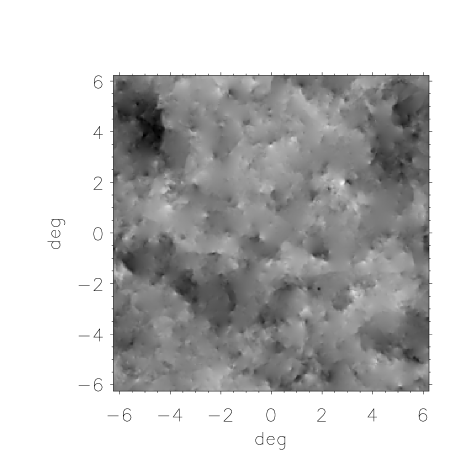
Figure 6: String map analysed in this paper.

In this section, we probe if our method is able to detect the non-Gaussian signature introduced by cosmic strings. To this end, we apply our method to the analysis of the string simulation shown in Fig. 6 (Bouchet et al., 1988). We first analyse the simulation without noise. In this way we can learn what happens when we have only the string map. After that we add different noise levels to see how the method is able to detect the strings.

Although in theory the correlation matrix depends only of the power spectrum and the beam (see expression 3), the (finite) pixel size of the real string map we are analysing and the irregular coverage of the visibility plane could introduce noticeable imprecisions. The correlation matrix of the strings is then calculated using Gaussian maps simulated with the same pixel size: we calculate the power spectrum of the string real map and construct Gaussian real maps with this power spectrum (we use 40000 Gaussian simulations). From these Gaussian maps we calculate the corresponding visibility values (expression 3). The correlation of these visibility simulations is that used for the analysis of the strings. Note that in the expression (3) there is no hypothesis concerning the statistic of the temperature field. The only hypothesis is the homogeneity of the field.

The template observation of the VSA is the same as in previous sections (895 binned visibilities in 9$\lambda$ cells).

6.2.1 Noiseless Map of Strings

In this case we diagonalize the correlation matrix of the signal because we do not have noise. With this diagonalization we decorrelate the data in a similar way as is done in sections 3.1 and 3.2.

We analyse the real and imaginary parts of the visibilities obtained from the string map without noise. The values found for the statistics are: $U_{1}^{2}\simeq 1.4\cdot 10^{3}$, $U_{2}^{2}\simeq 3.4\cdot 10^{8}$, $U_{3}^{2}\simeq 2.9\cdot 10^{13}$ and $U_{4}^{2}\simeq 4.4\cdot 10^{18}$. The estimated moments, $\hat{\mu}_{\alpha}$, are $\hat{\mu}_{1}\simeq-0.89$, $\hat{\mu}_{2}\simeq 6.2\cdot 10^{2}$, $\hat{\mu}_{3}\simeq-3.1\cdot 10^{5}$ and $\hat{\mu}_{4}\simeq 2.5\cdot 10^{8}$. These values are clearly incompatible with a Gaussian realization. The $y_{i}$ quantities (see expression 6) associated with the real parts of the string visibilities are shown in the Fig. 7 (those associated with the imaginary parts have similar features). Every $y_{i}$ has an associated signal eigenvalue $E_{i}$ whose value decreases with $i$. We see, then, that for the strings the absolute value (or amplitude) of $y_{i}$ grows when $E_{i}$ decreases (this explains why the moments $\hat{\mu}_{\alpha}$ are so large). This feature shows that the $y_{i}$ are not well decorrelated or normalized.

We analyse a Gaussian map with the same procedure. Figure 8 shows the resulting $y_{i}$ quantities for this Gaussian case. We see that they have a width of order of unity. Thus, we conclude that the behaviour of Fig. 7 is a feature of the non-Gaussianity of the string signal. The fact that the $y_{i}$ quantities are not well decorrelated or normalized indicates that we are not able to estimate their correlation matrix accurately. This seems to be because we have a model with a very large cosmic variance, and the correlation matrix (or equivalently the power spectrum) cannot be well estimated from only one realization. Moreover, we are estimating the power spectrum with the expression that maximizes the likelihood under the hypothesis of Gaussianity for the temperature field (Bond et al., 2000). But the temperature field is not Gaussian for the strings, and so the estimated power spectrum for the strings (that which maximizes the likelihood in this case) can differ from the one we are using. For a study of the dependence of the power spectrum on non-Gaussianity see Amendola (2002).

In the Gaussian case, however, we are able to calculate the power spectrum and then we decorrelate and normalize the visibilities properly. In this way, the $y_{i}$ quantities have a width equal to unity, i.e. $\langle y_{i}^{2}\rangle=1$, as shown in Figure 8. Summarizing, when there is no noise, in principle we should detect the strings by means of all the $U_{i}^{2}$ statistics (even $U_{1}^{2}$ and $U_{2}^{2}$) because their values are not compatible with a $\chi_{1}^{2}$ distribution (see Table 1).

Figure 7: Values of $y_{i}$ associated with the real part of the visibilities for an observation of the string map presented in Fig. 6 using our VSA template without adding noise.

Figure 8: Same as in Fig. 7, but for a simulated Gaussian CMB map.

Finally, we have applied the smooth tests of goodness-of-fit developed by Neyman to the phases of the visibilities of the noiseless map of strings (section 3.3). The $U_{i}^{2}$ values are: $U_{1}^{2}=3.64$ ($94.36\%$), $U_{2}^{2}=4.59$ ($96.78\%$), $U_{3}^{2}=0.32$ ($42.84\%$) and $U_{4}^{2}=0.13$ ($28.16\%$). And for the $S_{i}$ statistics: $S_{1}=3.64$ ($94.36\%$), $S_{2}=8.23$ ($98.37\%$), $S_{3}=8.55$ ($96.41\%$) and $S_{4}=8.68$ ($93.04\%$). The probability of obtaining a lower or equal statistic value under the null hypothesis (the visibilities are Gaussian) is showed in parentheses.

In the following subsection we discuss the effect of Gaussian noise on the detectability of strings with our method.

6.2.2 String map with different noise levels

The features in Fig. 7 change when (Gaussian) noise is added. The behaviour for low values of $i$ remains unchanged because these values are associated with high signal-to-noise values so that these data are dominated by the signal. However, the behaviour for high $i$ is dominated by the noise (low signal-to-noise eigenvalues) so that the behaviour will resemble that of a Gaussian signal.

The analysis with different noise levels is given in Table 4 (noise corresponding to an integration time equal to $25\times 4$ hr) and Table 5 (noise corresponding to an integration time equal to $25\times 25\times 4$ hr). We have analysed 5000 simulations involving the string simulation plus a noise realization. The analysis is done for different cuts of the eigenvalues ($E^{\mathrm{cut}}$). The power to distinguish between a Gaussian distribution and the strings plus noise when the significance level is $5\%/1\%$ is shown in the tables.

Table 4: Power of the $U_{i}^{2}$ ($i=1,2,3,4$) statistics for simulated observations of the strings map using a noise level corresponding to an integration time of $25\times 4$ hr. The columns indicate the power in percentage when the significance level is $5\%/1\%$.

$E^{\mathrm{cut}}$	$U_{1}^{2}$	$U_{2}^{2}$	$U_{3}^{2}$	$U_{4}^{2}$
0.	5.16/0.82	5.72/1.20	4.92/1.00	4.50/0.98
0.1	3.72/0.58	6.00/0.86	2.28/0.36	1.70/0.28
0.2	3.10/0.30	4.16/0.44	1.70/0.24	1.20/0.34
0.3	5.10/0.66	3.36/0.22	1.48/0.26	1.24/0.30
0.4	1.46/0.14	1.78/0.12	1.08/0.36	1.28/0.30
0.5	1.00/0.10	2.04/0.08	0.80/0.18	0.90/0.22

Table 5: Power of the $U_{i}^{2}$ ($i=1,2,3,4$) statistics for simulated observations of the string map using a noise level corresponding to an integration time of $25\times 25\times 4$ hr. The columns indicate the power in percentage when the significance level is $5\%/1\%$.

$E^{\mathrm{cut}}$	$U_{1}^{2}$	$U_{2}^{2}$	$U_{3}^{2}$	$U_{4}^{2}$
0.	5.30/0.98	24.26/8.44	4.20/0.86	4.28/1.04
0.1	6.56/0.84	79.56/49.32	1.58/0.12	1.30/0.22
0.2	7.18/0.92	86.72/59.60	1.08/0.08	1.24/0.34
0.3	2.94/0.26	87.62/60.44	0.80/0.04	0.70/0.10
0.4	3.74/0.10	90.74/64.16	0.48/0.02	0.66/0.08
0.5	3.20/0.12	92.90/69.58	0.48/0.08	0.38/0.08

The results in Table 4 indicate that the VSA noise of a single field observed during $25\times 4$ hrs is too high for detecting the strings with our method. When the integration time is multiplied by 25 (Table 5) we start to detect the strings by means of the $U^{2}_{2}$ statistic. It is important to note that, even if the data were well decorrelated, the $U^{2}_{2}$ statistic would also be a indicator of non-Gaussianity. For example, given realizations of normalized and independent data with kurtosis $K\neq 0$, the mean value of $U^{2}_{2}$ is equal to $(K+2)/2\neq 1$. Another example of the use of $U^{2}_{2}$ to detect non-Gaussianity can be found in Aliaga et al. (2003b) in the formalism of the multinormal analysis.

As a test, we repeat the same procedure using a Gaussian simulation instead of the string map and, as expected, we obtain a negligible power.

6.3 $\chi^{2}$ simulations

Nowadays, non-Gaussian simulations constructed by the addition of a Gaussian field and its square have acquired a notable relevance because they could represent perturbations produced in several inflationary scenarios (for a review on the subject, see Bartolo et al. 2004 and references therein). The parameter which measures the coupling with the non-linear part is denoted by $f_{NL}$ and, then, an analysis to study the power of our method to detect this parameter seems to be very appropriate. Realistic simulations in the flat-sky approximation would require to develop appropriate software (see e.g. Liguori et al. 2003 for simulations on the full sphere), and this is beyond the scope of the present work. However, we can estimate the power of our method in detecting a non-zero $f_{NL}$ component using a simple approximation. We follow Aghanim et al. (2003), and we generate what they call “$\chi^{2}$ maps” by assuming that the observed temperature contrast field on sky ($\Delta(\mn@boldsymbol{x})\equiv\Delta T(\mn@boldsymbol{x})/T$) can be written as

$$\Delta(\mn@boldsymbol{x})=\Delta_{L}(\mn@boldsymbol{x})+f_{NL}(\Delta_{L}^{2}(\mn@boldsymbol{x})-\langle\Delta_{L}^{2}(\mn@boldsymbol{x})\rangle)$$

where $\Delta_{L}$ is the Gaussian (linear) component. In reality, this approximation is only valid in the Sachs-Wolfe regime (see e.g. Komatsu & Spergel 2001), but we use it as a toy model in our exercise of the study of the detection of the $f_{NL}$ parameter.

We first consider the ideal case where there is no instrumental noise, and we have analyzed different sets of simulations with $f_{NL}$ values $0$ (Gaussian case), $100$, $1000$ and $10000$. We have run $10000$ simulations for every case. Only the case with $f_{NL}=10000$ has been detected via the $U_{2}^{2}$ statistic. Fig. 9 shows the distribution function of the $U_{2}^{2}$ statistic for the Gaussian case (dashed boxes), compared with the corresponding one for the non-Gaussian case with $f_{NL}=10000$ (solid boxes). From here, we infer that the power of this statistic to discriminate between the non-Gaussian simulations and the Gaussian ones is about the $79\%$ ($72\%$) with a significance level of $5\%$ ($1\%$). Analysing the same previous simulations but adding the noise level corresponding to an observation time of $25\times 25\times 4$ hr, we find that the power of our statistic is reduced roughly by a factor 2.

Smith et al. (2004) constrained the $f_{NL}$ parameter by using the bispectrum of the VSA extended array data (note that this is exactly the same configuration that we have adopted to build our visibility template). With their definition of $f_{NL}$, they found an upper limit of 7000 with a confidence level of $95\%$. In the Sachs-Wolfe regime, this would correspond to a value of 31500 according to our $f_{NL}$ definition. However, this value can not be direclty compared with the one obtained in our work, because our model does not correspond to the realistic case which was considered in Smith et al. (2004).

Figure 9: Distributions of $U_{2}^{2}$ for the Gaussian case (dashed boxes) and for the non-Gaussian case with $f_{NL}=10000$ (solid boxes). The solid line is a $\chi^{2}_{1}$ function normalized to the number of simulations (10000 simulations). (For the sake of clarity, the histogram for the Gaussian case has been cut at the top.)

7 Discussion and Conclusions

In this paper we have presented a method of searching for non-Gaussianity in data from interferometric CMB observations, directly in the visibility space. This method can be adapted to other interferometric experiments (e.g. CBI and DASI) if we know the correlation matrices of the signal and of instrumental noise. Note that in this paper, we have dealt with decorrelated noise (which is usually the case for these experiments), but the case of correlated noise can be studied in an analogous way.

We have applied the method to work with the real and imaginary parts of the visibilities. The method tests whether they are Gaussian distributed. However, we have applied the method to the phases of the visibilities to test whether they are uniformly distributed, but we found that it is not very sensitive for detecting the kind of non-Gaussianity we have analysed here.

We have integrated the signal-to-noise formulation into the smooth goodness-of-fit tests. In this way we can deal only with the data dominated by the signal we want to analyse. In the text it is noted that the correlation matrices of the signal-to-noise eigenmodes and of the signal are descomposed as the product of a matrix and its transpose (subsection 3.1 and section 5). This decomposition is analogous to that of Cholesky. This latter decomposition is computationally faster than the one used here; however, the decomposition we use allows us to deal with better quality data, that is, with a higher signal-to-noise ratio. The analysis with the Cholesky decomposition takes every eigenvalue; that is, $E^{\mathrm{cut}}=0$.

It is important to stress that smooth goodness-of-fit tests do not require the data to be on a regular grid, but can be applied to any data set. In that sense the test is perfectly adapted to interferometric data because the coverage of the $UV$ plane is neither regular nor complete. The method could therefore also be applied by selecting those visibilities in a certain $UV$ range, thus allowing study of the non-Gaussianity as a function of angular scale. In addition, although the method has been presented here as a tool to study the non-Gaussian properties of the sky signal, it could also be used as a powerful diagnostic for detecting systematics in the data, as we pointed out in Section 6.1. For short integration periods, a stack of visibilities will be dominated by instrumental noise, so this method could be used to trace the presence of spurious signals in the data (e.g. those comming from cross-talk between antennas), or to study the correlation properties of the noise.

Summarizing, to study the power of our method in detecting non-Gaussian signals on the sky, we have analysed three kinds of simulations. First we have analysed non-Gaussian visibilities created by inserting some degree of skewness and kurtosis ($S=K=1$) with the Edgeworth expansion directly in Fourier space. Using the VSA as a reference experiment, we have shown the performance of the method in detecting those levels of non-Gaussianity in the data with realistic values of the integration time for this experiment. All these results can be easily adapted to other instruments, just by rescaling the integration times according to the square of the ratio of the different sensitivities. In addition, we have also shown the performance of the test in the detection of the non-Gaussian signal introduced by cosmic strings. Even though those kind of signals are usually detected using real-space statistics or wavelets (Hobson et al., 1999; Barreiro & Hobson, 2001), we have demonstrated that the signal-to-noise eigenmodes approach allows us to detect them because the method is very sensitive to the characterization of the covariance matrix. In this particular case, due to the non-Gaussian nature of the strings, a complete decorrelation can not be achieved and the statistics show huge deviations with respect to the Gaussian case. For the case of the VSA, this translates into the fact that cosmic strings can hardly be detected in single-field observations (integration times of $25\times 4$ hr), but they could be detected (if present) using this method, given the current sensitivity achieved by the whole data set published by the VSA team (with a sensitivity of $\sim$25 $\times 25\times 4$ hr integration). Finally, we have studied the power of the method to detect a non-zero $f_{NL}$ component in a toy model based on $\chi^{2}$ maps.

Appendix A Bispectrum of the Edgeworth expansion

Suppose a square real map of pixel coordinates $\mn@boldsymbol{x}$ and pixel data $y_{\mn@boldsymbol{x}}$. These values are generated via the Edgeworth expansion such that they are independent, normalized and have skewness $S$. The map has $N_{\mathrm{side}}$ pixels on a side and the area of the pixel is $\Delta^{2}$. We now perform its Fourier transform:

$$\tilde{a}_{\mn@boldsymbol{k}}=\Delta^{2}\sum_{\mn@boldsymbol{x}}y_{\mn@boldsymbol{x}}e^{i\mn@boldsymbol{k}\mn@boldsymbol{x}}$$

whose bispectrum is

$$\langle\tilde{a}_{\mn@boldsymbol{k_{1}}}\tilde{a}_{\mn@boldsymbol{k_{2}}}\tilde{a}_{\mn@boldsymbol{k_{3}}}\rangle=\Delta^{6}\sum_{\mn@boldsymbol{x_{1}}\mn@boldsymbol{x_{2}}\mn@boldsymbol{x_{3}}}\langle y_{\mn@boldsymbol{x_{1}}}y_{\mn@boldsymbol{x}_{2}}y_{\mn@boldsymbol{x}_{3}}\rangle e^{i\mn@boldsymbol{k}_{1}\mn@boldsymbol{x}_{1}}e^{i\mn@boldsymbol{k}_{2}\mn@boldsymbol{x}_{2}}e^{i\mn@boldsymbol{k}_{3}\mn@boldsymbol{x}_{3}}$$

Taking into account that $y_{\mn@boldsymbol{x}}$ are independent and $\langle y_{\mn@boldsymbol{x}}^{3}\rangle=S$ we have

$$\langle\tilde{a}_{\mn@boldsymbol{k_{1}}}\tilde{a}_{\mn@boldsymbol{k_{2}}}\tilde{a}_{\mn@boldsymbol{k_{3}}}\rangle=N_{\mathrm{side}}^{2}\;\Delta^{6}\;S\;\delta_{\mn@boldsymbol{k}_{1}+\mn@boldsymbol{k}_{2}+\mn@boldsymbol{k}_{3},\mn@boldsymbol{0}}$$

where $\delta_{\mn@boldsymbol{k}_{1},\mn@boldsymbol{k}_{2}}=N_{\mathrm{side}}^{-2}\sum_{\mn@boldsymbol{x}}e^{i(\mn@boldsymbol{k}_{1}-\mn@boldsymbol{k}_{2})\mn@boldsymbol{x}}$ is the Kronecker delta. The Fourier modes could be normalized to the desired spectrum: $a_{\mn@boldsymbol{k}}=C_{k}^{1/2}\tilde{a}_{\mn@boldsymbol{k}}/(N_{\mathrm{side}}\Delta^{2})$ such that $\langle a_{\mn@boldsymbol{k}}a_{\mn@boldsymbol{k}}^{*}\rangle=C_{k}\delta_{\mn@boldsymbol{k}_{1},\mn@boldsymbol{k}_{2}}$. Finally, the (normalized) bispectrum is given by

$$\frac{\langle a_{\mn@boldsymbol{k}_{1}}a_{\mn@boldsymbol{k}_{2}}a_{\mn@boldsymbol{k}_{3}}\rangle}{\langle|a_{\mn@boldsymbol{k}_{1}}|^{2}\rangle^{1/2}\langle|a_{\mn@boldsymbol{k}_{2}}|^{2}\rangle^{1/2}\langle|a_{\mn@boldsymbol{k}_{3}}|^{2}\rangle^{1/2}}=\frac{S}{N_{\mathrm{side}}}\delta_{\mn@boldsymbol{k}_{1}+\mn@boldsymbol{k}_{2}+\mn@boldsymbol{k}_{3},\mn@boldsymbol{0}}.$$

Note that the Gaussianity associated to the third moment in the Fourier space is reduced by a factor $N_{\mathrm{side}}$ compared to that in real space.

Appendix B Skewness and kurtosis of a given eigenmode from the Edgeworth expansion

When we introduce some degree of non-Gaussianity (skewness or kurtosis) by means of the Edgeworth expansion in the visibilities, it is clear that each eigenmode will show a different degree of non-Gaussianity which will depend on the associated signal-to-noise eigenvalue. This relation can be obtained as follows.

As it is explained in the main text, we generate a realization of independent values $y_{j}$ with zero mean, unit variance, and skewness and kurtosis $S$ and $K$, respectively. As in subsection 5, the real parts of the visibilities are $V_{i}^{R}=\sum_{j}L_{s,ij}^{R}y_{j}$. The imaginary parts are generated in an analogous way. After that, we add the corresponding different noise levels and decorrelate the data by using the transformation given by equation (5). Then, bearing in mind the definition of the $E_{k}$ quantities, it can be easily demonstrated that for the final decorrelated and normalized data we have

$$\langle y_{k}^{3}\rangle=\bigg{(}\frac{E_{k}}{E_{k}+1}\bigg{)}^{3/2}S\quad;\quad\langle y_{k}^{4}\rangle-3=\bigg{(}\frac{E_{k}}{E_{k}+1}\bigg{)}^{2}K.$$

As one would expect, the skewness and the kurtosis are lost if the (Gaussian) noise dominates the data ($E_{k}\ll 1$). In contrast, the skewness and the kurtosis are preserved for the case $E_{k}\gg 1$. In the previous expressions, the angled brackets ($\langle\cdot\rangle$) denote an average over realizations.

References

- Aghanim et al. (2003) Aghanim, N., Kunz, M., Castro, P. G., & Forni, O. 2003, A&A, 406, 797
- Aliaga et al. (2003a) Aliaga A. M., Martínez-González E., Cayón L., Argüeso F., Sanz J. L., Barreiro R. B., 2003a, New Astronomy Reviews, 47, 821
- Aliaga et al. (2003b) Aliaga A. M., Martínez-González E., Cayón L., Argüeso F., Sanz J. L., Barreiro R. B., Gallegos J. E., 2003b, New Astronomy Reviews, 47, 907
- Amendola (2002) Amendola, L. 2002, ApJ, 569, 595
- Balbi et al. (2000) Balbi, A. et al. 2000, ApJ, 545, L1
- Barreiro & Hobson (2001) Barreiro, R. B. & Hobson, M. P. 2001, MNRAS, 327, 813
- Bartolo et al. (2004) Bartolo, N., Komatsu, E., Matarrese, S., & Riotto, A. 2004, Phys. Rep., accepted (astro-ph/0406398)
- Bond (1995) Bond, J. R. 1995, Phys. Rev. Lett., 74, 4369
- Bond et al. (2000) Bond, J. R., Jaffe, A. H. & Knox, L. 2000, ApJ, 533, 19
- Bouchet et al. (1988) Bouchet, F. R., Bennett, D. P. & Stebins, A. 1988, Nat, 335, 410
- Cayón et al. (2003a) Cayón, L., Martínez-González, E., Argüeso, F., Banday, A.J. & Górski, K.M., 2003a, MNRAS, 339, 1189
- Cayón et al. (2003b) Cayón, L., Argüeso, F., Martínez-González, E. & Sanz J. L. 2003b, MNRAS, 344, 917
- Chiang et al. (2003) Chiang, L., Naselsky, P. D., Verkhodanov, O. V. & Way, M. J. 2003, ApJ, 590, L65
- Cox & Hinkley (1974) Cox D. R. & Hinkley, D. V. 1974, Theoretical Statistics (London: Chapman & Hall)
- Cruz et al. (2004) Cruz, M., Martínez-González, E., Vielva, P., & Cayón, L. 2004, MNRAS, in press (astro-ph/0405341)
- Dickinson et al. (2004) Dickinson, C. et al. 2004, MNRAS, 353, 732
- Eriksen et al. (2004a) Eriksen, H. K., Hansen, F. K., Banday, A. J., Górski, K. M., & Lilje, P. B. 2004a, ApJ, 604, 14
- Eriksen et al. (2004b) Eriksen, H. K., Novikov, D. I., Lilje, P. B., Banday, A. J., & Górski, K. M. 2004b, ApJ, 612, 64
- Grainge et al. (2003) Grainge, K. et al. 2003, MNRAS, 341, L23
- Guth (1981) Guth, A. H., 1981, Phys. Rev. D., 23, 347
- Hanany et al. (2000) Hanany, S. et al. 2000, ApJ, 545, L5
- Hobson et al. (1999) Hobson, M. P., Jones, A. W. & Lasenby, A. N. 1999, MNRAS, 309, 125
- Hobson & Maisinger (2002) Hobson, M. P. & Maisinger, K. 2002, MNRAS, 334, 569
- Komatsu & Spergel (2001) Komatsu, E. & Spergel, D. N. 2001, Phys.Rev.D, 63, 063002
- Komatsu et al. (2003) Komatsu, E. et al. 2003, ApJS, 148, 119
- Lay & Halverson (2000) Lay, O. P. & Halverson, N. W. 2000, ApJ, 543, 787
- Leitch et al. (2002) Leitch, E. M. et al. 2002, ApJ, 568, 28
- Liguori et al. (2003) Liguori, M., Matarrese, M. & Moscardini, L. 2003, ApJ, 597, 57
- Martínez-González et al. (2002) Martínez-González, E., Gallegos, J. E., Argüeso, F., Cayón, L. & Sanz, J. L. 2002, MNRAS, 336, 22
- Melhuish et al. (1999) Melhuish, S. J., Dicker, S., Davies, R. D., Gutierrez, C. M., Watson, R. A., Davis, R. J., Hoyland, R. & Rebolo, R. 1999, MNRAS, 305, 399
- Neyman (1937) Neyman, J. 1937, Skandinavisk Aktuarietidskrift, 20, 150
- Padin et al. (2001) Padin, S. et al. 2001, ApJ, 549, L1
- Park (2004) Park, C. 2004, MNRAS, 349, 313
- Rayner & Best (1989) Rayner, J. C. W. & Best D. J. 1989, Smooth Tests of Goodness of Fit (New York: Oxford University Press)
- Rayner & Best (1990) Rayner, J. C. W. & Best, D. J. 1990, International Statistical Rev., 58, 9
- Rocha et al. (2001) Rocha, G., Magueijo, J., Hobson, M. & Lasenby, A., 2001, Phys. Rev. D., 64, 063512
- Savage et al. (2004) Savage, R. et al. 2004, MNRAS, 349, 973
- Smith et al. (2004) Smith, S. et al. 2004, MNRAS, 352, 887
- Taylor et al. (2003) Taylor, A. C. et al. 2003, MNRAS, 341, 1066
- Vielva et al. (2004) Vielva, P., Martínez-González, E., Barreiro, R. B., Sanz, J. L., & Cayón, L. 2004, ApJ, 609, 22
- Watson et al. (2003) Watson, R. A. et al. 2003, MNRAS, 341, 1057
- White et al. (1999) White, M., Carlstrom, J. E., Dragovan, M., & Holzapfel W. L. 1999, ApJ, 514, 12