Hybrid Simulation of Cosmic Ray Air Showers

Abstract

Air shower simulations are essential for interpreting data from cosmic ray experiments. At highest energies though, a microscopic treatment of a whole shower is not possible any more, since it would require a huge amount of CPU-time. We review hybrid approaches of air shower simulation which try to overcome this problem without giving rise to artificial fluctuations as generated by the thinning algorithm.

1 Introduction

Ultra-high energy cosmic rays (UHECR) are currently of great interest. One still ignores the nature of these particles, acceleration mechanisms and possible sources. Direct measurements at these energies are impossible due to a very low flux. Upon entering the atmosphere, cosmic rays induce extensive air showers (EAS), cascades of particles produced by collisions of the primary and subsequent secondaries with air nuclei. Experiments measure these showers and try to deduce properties of the primary particle from properties of the shower. One can therefore consider the atmosphere as a huge detector in which a primary cosmic ray is absorbed and observed.

There are basically two types of experimental set-ups. Ground arrays (i.e. AGASA, Auger) measure the density of charged particles on the ground. The lateral distribution function (LDF) is studied to deduce the energy. One can estimate the arrival direction from the different trigger-times of the detectors as the shower front passes through the array. The other kind are optical detectors. They collect the light emitted by fluorescence of nitrogen molecules, which are excited by the flux of charged particles going through the atmosphere. They measure therefore directly the longitudinal profile of a shower. Both types of experiments have advantages and drawbacks. Ground arrays have a high duty cycle and are not very sensitive to details of the atmosphere. Fluorescence experiments depend somewhat less on models, but are influenced by atmospheric fluctuations and have a duty cycle of typically 10%.

For both set-ups, reconstruction of primary properties depends on how good one understands the interactions in the atmosphere. Air shower simulations are therefore crucial for cosmic ray physics as they are needed for interpretation of the data. A major difficulty is that no experimental data from accelerators is available at these energies. LHC is still three orders of magnitudes (lab. system) lower than the currently highest energies measured. Another problem is that air shower development is dominated by forward scattering, since most energy is carried by the leading particles, but accelerators measure mostly at mid-rapidity. Also, the targets are light nuclei, commonly less well studied. Therefore, physics has to be extrapolated into unknown regions (energy and phase-space) which makes interpretation of data less precise. On the other hand, one can argue that cosmic rays provide a unique opportunity to study physics at high energies that may never be reached by accelerator experiments.

Air showers develop rapidly in the atmosphere. A rule of thumb is that the number of charged particles at the maximum of the longitudinal profile is about 60% of the energy measured in GeV; a $10^{11}$ GeV shower has about 60 billion particles. Hence, microscopic simulations seem quite impossible. E.g., a $10^{10}$ GeV shower would take about a year to compute on current CPUs. The thinning algorithm [1] reduces the CPU time but introduces artificial fluctuations. Hybrid simulations [2] try to solve this problem by following the high energy part of an air shower in detail, and using efficient approximations below a given threshold.

2 The thinning problem in microscopic treatment of air shower simulations

Current air shower simulations use the thinning algorithm in order to limit the computation time. The original idea is to follow only one particle of all secondaries below a given threshold $E_{th}=f_{th}E_{0}$, chosen with the probability $p_{i}=E_{i}/E_{\rm tot}$. Neglected particles are compensated by attributing a higher weight $w_{i}=1/p_{i}$ to the chosen particle. In principle, the probability of some particle below the threshold to be followed can be an arbitrary function, but the weight attributed has to be $1/p_{i}$. Statistical thinning means $p_{i}=E_{i}/E_{\rm tot}$ (as above, but the number of followed particles is not fixed to one). Further refinements are possible by imposing a weight limit on the algorithm, or not to thin beyond a given distance from the shower axis. The disadvantage of thinning is that it introduces artificial fluctuations, and one has to be careful to control these.

The hybrid approach tries to overcome these problems by computing the sub-showers of particles efficiently instead of discarding these.

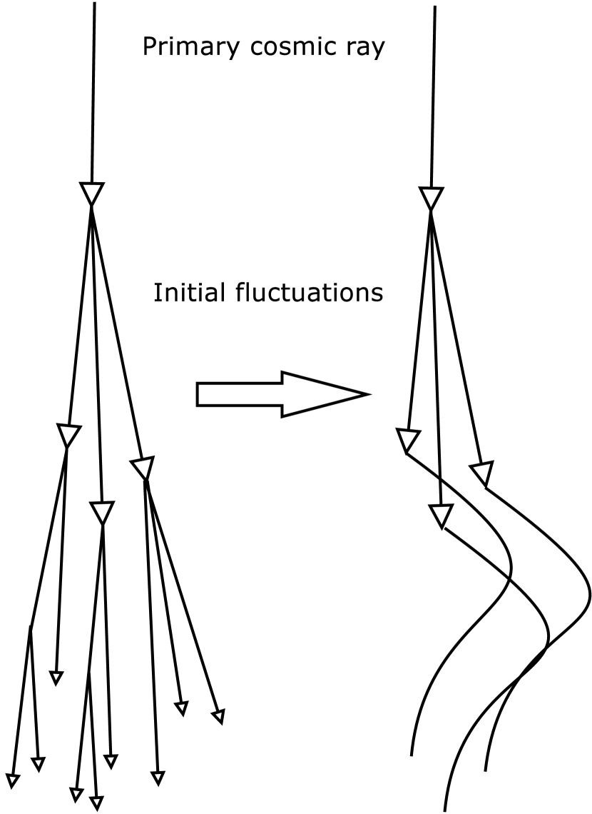
Figure 1: Principle of the hybrid approach: compute sub-showers with efficient algorithms.

3 Hybrid approaches

As mentioned, hybrid methods replace sub-threshold particles with the sub-showers induced by them. We are going to discuss two different approaches, where these sub-showers are obtained from a shower library or the solution of cascade equations. They differ also in the fact, that the former replaces a fluctuating shower whereas the latter solves for mean sub-showers.

3.1 Bartol approach to hybrid simulations

An obvious choice is to implement a data base of pre-simulated showers. During the simulation, all sub-showers below a given energy threshold are replaced with a sample from this data base. The Bartol [7] approach consists of a shower library of pion-initiated showers for different injection depths, energies and zenith angles. Nucleons are followed by Monte-Carlo method, whereas kaons are treated to behave as pions with respect to interaction. The resulting longitudinal profiles are then fitted to a Gaisser-Hillas function, and the parameters are recorded. In addition, the number of muons at ground level for different energy thresholds is stored. The library itself is built with a boot-strap method: Starting from low energy, the pre-simulated showers are used for the computation of higher energies. During the simulation of a given shower, each particle falling below the threshold $E_{\rm th}=0.01E_{0}$ is replaced with a sub-shower sampled from the data base. Note that these sub-showers are not average profiles but account fully for fluctuations even below the hybrid threshold.

3.2 Hybrid approach with cascade equations

Cascade equations are one-dimensional transport equations which are solved numerically. The solution is a mean shower profile without any fluctuations. Given a number of particles $h_{n}(E,X)dE$, of type $n$, at given altitude $X$ and energy $E$, the probability for interaction and decay is

$$\frac{\partial h_{n}(E,X)}{\partial X}=-h_{n}(E,X)\left(\frac{1}{\lambda_{n}(E)}+\frac{d_{n}}{E\rho(X)}\right)$$ (1)

with $\lambda$ being the mean free path of the particle as a function of the energy, $\rho$ being the density of the air, and $d_{n}=m_{n}/(c\tau_{n})$ being the decay constant ($E/d_{n}$ is the decay length in the lab. system).

Accounting for particles produced at higher energies gives rise to the following system of hadronic cascade equations [5]:

$$\frac{\partial h_{n}(E,X)}{\partial X}=-h_{n}(E,X)\left[\frac{1}{\lambda_{n}(E)}+\frac{d_{n}}{E\rho(X)}\right]$$ (2)

$$+\sum_{m}\int_{E}^{E_{\mathrm{max}}}h_{m}(E^{\prime},X)\left[\frac{W_{mn}(E^{\prime},E)}{\lambda_{m}(E^{\prime})}\right.$$

$$\left.+\frac{d_{m}D_{mn}(E^{\prime},E)}{E^{\prime}\rho(X)}\right]dE^{\prime}~{}~{}.$$

The functions $W_{mn}(E^{\prime},E)$ are the energy-spectra $\frac{dN}{dE}$ of secondary particles of type $n$ in a collision of hadron $m$ with air-molecules. $D_{mn}(E^{\prime},E)$ are the corresponding decay-functions. Equation (2) is a typical transport equation with a source term. The first term with the minus-sign accounts for particles disappearing by collisions or decays, whereas the source term accounts for production of secondary particles by collisions or decays of particles at higher energies.

The initial condition for the primary cosmic ray is given by

$$h_{n}(E,X=X_{m})=\delta_{nm}\delta(E-E_{m}).$$ (3)

When using the hybrid approach, the initial condition is a superposition of all particles $E<E_{th}$ produced above the threshold.

3.3 Low energy source functions

At low energies, the three-dimensional spread of particles becomes important. For the computation of the longitudinal profile only, one can apply corrections to the one-dimensional cascade equations in order to account for neglecting the lateral expansion. This is done in the conex model [4].

For the computation of lateral distribution functions one can switch back to the Monte-Carlo scheme. Particles are generated from the so-called source function,

$$\frac{\partial h^{\rm source}_{n}(E,X)}{\partial X}=\sum_{m}\int_{E_{\min}}^{E_{\max}}h_{m}(E^{\prime},X)$$ (4)

$$~{}~{}~{}~{}~{}~{}~{}~{}~{}~{}~{}~{}~{}\left[\frac{W_{mn}(E^{\prime},E)}{\lambda_{m}(E^{\prime})}\right.+\left.\frac{d_{m}D_{mn}(E^{\prime},E)}{E^{\prime}\rho(X)}\right]dE^{\prime}\,.$$

Source functions are used in the seneca model [6] and by Dedenko et al. [3]. Particles are generated according to (4) and placed along the shower axis.

The source function contains a certain energy

$$E_{\rm tot}=\sum_{n}\int_{E_{\min}}^{E_{\max}}dEdX\frac{E\partial h^{\rm source}_{n}(E,X)}{\partial X}~{},$$

which should be used to produce secondary particles. By choosing a fraction $f$ of this energy, one determines the weight of the secondaries. Ideally this should be equal to one, but this would still take too much of CPU power. However, once determined, the weight stays constant even in the subsequent tracking with MC method. This is an advantage over the thinning method where the weight of particles is more difficult to control.

The choice of the energy threshold $E_{\max}$, where to switch back from CE to MC is crucial. A lower value is desirable for computation speed, whereas a higher value might be needed to achieve the desired precision for the lateral distribution function. The best value to choose depends therefore also on the observable to be computed. For example, for longitudinal profiles the lateral spread of muons is not important, and one can choose a lower transition energy.

3.4 Electromagnetic showers

The electromagnetic part of the shower can be treated in a similar way. In seneca, pre-simulated sub-showers for a 2.5 g/cm² thick layer of air are stored in a table. The energies are discretized in ten bins per decade $E_{i}=10^{i/10}$. The table is then a matrix $V_{ij}^{mn}$, where the indices $i,j$ represent primary and secondary energies, $m,n$ stand for the particle types, photons and electrons/positrons. If we have $g_{i}^{n}(X)$ particles of type $n$ and energy $E_{i}$, the corresponding spectrum at $X+\Delta X$ is

$$g_{i}^{n}(X+\Delta X)=\sum_{j,m}V_{ij}^{nm}g_{j}^{m}(X)~{}~{}.$$

Dedenko et al., Lagutin et al. [8], as well as conex choose to implement cascade equations in a similar way to (2) for all electromagnetic interactions, i.e. pair production, bremsstrahlung, etc. At low energies, conex implements a higher effective path length, in order to correct for the neglected transverse dimensions. In seneca one can apply a table of pre-simulated sub-showers. This way, the longitudinal profile can be calculated in a quick way, using the slow MC method only for initial fluctuations.

4 Results and Comparisons

4.1 Internal checks

Figure 2: A single mean CE shower compared with 1000 averaged MC-showers ($10^{-5}$ thinning).

Figure 3: Lateral distributions for electrons/positrons, muons and photons. The cut-off energies are 50 MeV for muons and 1 MeV for the EM-particles.

Figure 4: Energy spectra for both simulation methods.

Figure 5: The spread of $X_{\max}$ as a function of the hybrid threshold $f$.

Figure 6: Mean $X_{\max}$ of conex and seneca compared with corsika results. The Seneca proton result for neXus 3.97 has been computed with CE only ($X_{\max}$ of a mean shower).

Precision is crucial for the hybrid approach. Any lack of precision will appear in the solution systematically. Therefore it is necessary to confirm whether CE and MC give the same results. Since the cascade equations give as result a mean shower, we compare the longitudinal profile of one CE shower to the average of 1000 MC generated showers. Here we do not use MC for the initial part, i.e. $f=1$. The agreement of the two curves is shown in Fig. 2.

Since the CE approach is ideal to compute an average shower, one might ask how good the maximum of a mean shower describes the mean of fluctuating showers, as measured by experiments. Assuming the shower profiles are described by functions $f_{i}(x)$, the mean shower is

$$f(x)=\frac{1}{N}\sum_{i=1}^{N}f_{i}(x)~{}.$$ (5)

The maximum is defined by $f^{\prime}(x)=0$ so $f^{\prime}(X_{\max})=0$ and $f_{i}^{\prime}(X_{\max,i})=0$. Expanding each profile $i$ around its maximum yields

$$f_{i}(x) = f_{i}(X_{\max,i})$$ (6)

$$+\frac{f_{i}^{\prime\prime}(X_{\max,i})}{2}(x-X_{\max,i})^{2}$$

$$+...$$

Differentiating to find the maximum gives

$$0 = f^{\prime}({X_{\max}})=\frac{1}{N}\sum f_{i}^{\prime}(X_{\max})$$ (7)

$$= \frac{1}{N}\sum{f_{i}^{\prime\prime}(X_{\max,i})}(X_{\max}-X_{\max,i})~{},$$

which leads to

$$X_{\max}=\langle X_{\max,i}\rangle~{}{\rm for}~{}f_{i}^{\prime\prime}(X_{\max,i})=c~{}~{}.$$ (8)

So, if the curvature at $X_{\max,i}$ is approximately a constant, the maximum of a mean shower corresponds to the mean of maxima. Simulations show that this relationship (8) is valid within a few g/cm². Hence, for a quick estimate one can use a mean shower computed with the CE approach, instead of doing hundreds of fluctuating showers.

The same does not hold for the shower size, $S_{\max}$. Evaluating formula (6) at $X_{\max}$ yields

$$S_{\max} = f(X_{\max})=\langle S_{\max,i}\rangle$$ (9)

$$+ \frac{c}{2}\left(\langle X_{\max,i}^{2}\rangle-\langle X_{\max,i}\rangle^{2}\right)$$

$S_{\max}$ of a mean shower is smaller than the mean of $S_{\max}$ of many showers, since $c$ is negative. Because of energy conservation, we expect the mean shower to be somewhat wider than on average (larger $\Lambda$ in the Gaisser-Hillas formula). In that sense, a mean shower is not a typical shower, but it can be used to get a good estimate of the mean $X_{\max}$.

4.2 Lateral Distribution Functions

A check of lateral distribution functions (LDF) is shown in Fig. 3. The densities for electrons/positrons, muons, and photons agree with the MC simulated spectra of a vertical $10^{19}$ eV proton induced shower. In this example we compare two fluctuating showers as opposed to comparing the average behavior. The high energy part of the shower is calculated in the same way in both the MC and the CE simulation. Technically this is achieved by implementing a high energy particle stack and using the same seed for the pseudo-random number generator. The high energy stack takes care that the sequence of random numbers is exactly the same until the first particle below the threshold appears in the calculation.

An important parameter for the LDFs is the threshold in energy for switching back to the MC method. We choose $10$ GeV for electromagnetic cascades and $10$ TeV for the hadronic part. This relatively high value is necessary to reproduce correctly the lateral spread of the muons.

4.3 Energy Spectra

Energy spectra of all particles are directly calculated in the CE. An example for energy spectra at 600 g/cm² is shown in Fig. 4. Note the differences in K-short and K-long below $10^{5}$ GeV; this is the energy region where decays of K-shorts start dominate over interaction.

4.4 Fluctuations

An important check for the hybrid approach is whether it can reproduce natural fluctuations in the $X_{\max}$ distribution. Fig. 5 shows the spread $\sigma=\sqrt{\langle X_{\max}^{2}\rangle-\langle X_{\max}\rangle^{2}}$ as a function of the threshold $f$ (below $E=fE_{0}$ cascade equations are used). As of $f=0.01$ the spread seems to converge. Interestingly, already $f=0.99$ reproduces 90% of the spread, i.e. the very first interaction is responsible for most of the fluctuations.

4.5 Shower maximum

A comparison with the well tested corsika[9]  model is given in Fig. 6. Since the physics content in terms of external models is the same, the hybrid approaches should give similar results. qgsjet01 [10], sibyll 2.1[11] and neXus 3.97[12] are used as high energy hadronic models in the framework of conex and seneca.

When computing an iron induced shower with CE, one does not need any additional tables for nucleus primaries, if the energy per nucleon is above the initial fluctuation threshold. For direct computation of a mean shower, one would have in principle to do tables for all possible nucleus primaries up to $A=56$. In that case, it is more reasonable to average over many iron-air collisions (such that no nuclei are left) before solving the transport equations.

4.6 Arrival time

Figure 7: Arrival time distributions of photons and the corresponding maximum weight in a given bin. The peak in the MC figure is due to a single particle with a huge weight.

Arrival times are interesting, since modern experiments try to extract information about the primary via e.g. the rise time. Here, the thinning procedure has a great disadvantage, since the weight of a given particle can be dominant for the signal, as shown in Fig. 7. The largest peak is due to a single particle with a huge weight. Particles generated from the source function have a constant weight, which is adjustable. However, refined thinning algorithms have a weight limit, with which the maximum weight of a particle can be defined.

This is one example where the technique of CE has a useful side-effect, other than the main advantage of reduced CPU-time.

4.7 Very inclined showers

Figure 8: A $80^{\circ}$ inclined $10^{19}$ eV proton induced shower for pure MC and the hybrid (CE) method.

Inclined showers are of great interest for water tank detectors as in the Auger observatory. These are very different from near-vertical showers, due to a huge path-length. For 80^∘ inclined showers, we have 6 times the thickness of the atmosphere, and at $90^{\circ}$ 36 times. The electromagnetic part is almost absorbed in the atmosphere after some 2000 g/cm²; only muons continue to propagate with few interactions due to energy-loss, decays, bremsstrahlung, etc. The result is a relatively flat profile, see Fig. 8. The accompanying electrons/positrons and photons come from interactions and decays of muons. When calculating such a profile with CE, we solve only up to 2000 $g/cm^{2}$ slant depth, since beyond that value muons dominate the shower. The profiles from the MC and CE approaches agree nicely. But since the distance is large, a small error in the creation of hadrons from the source function could result in a wrong lateral shape. This is shown in Fig. 9, where we plot the muon density at ground level in the shower plane. The deflection of positive and negative muons due to the geomagnetic field is clearly visible. This is important to take into account when analyzing experimental data from ground arrays. Fig. 9(top) shows the MC event and Fig. 9(middle) a corresponding result with CE. Since the particles are placed with zero angle along the shower axis, the pattern looks distinctly different. In Fig. 9(bottom) a hybrid calculation is shown, where a mean transverse momentum is applied to all particles generated by the source function. A value of $p_{t}\approx 0.3$ GeV seems to be sufficient to reproduce the right pattern.

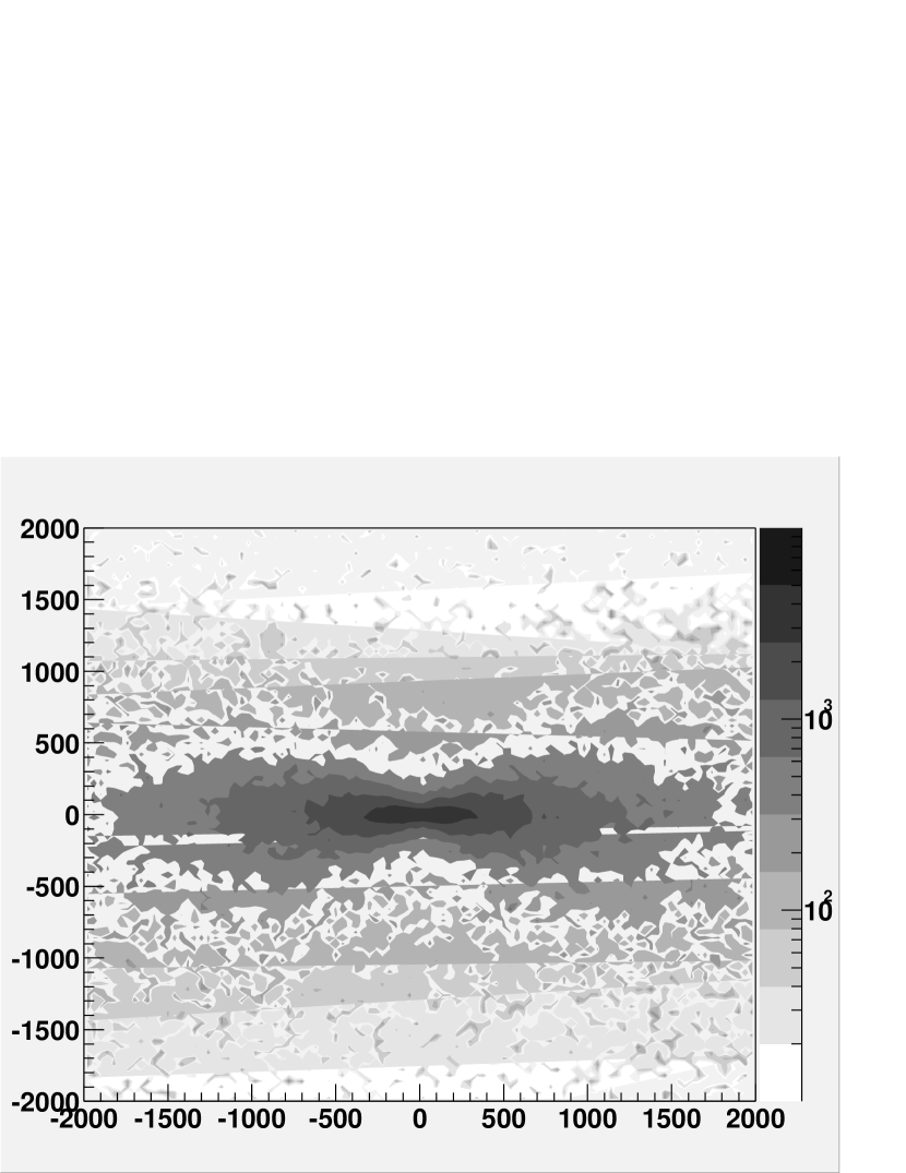
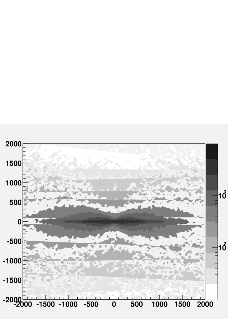
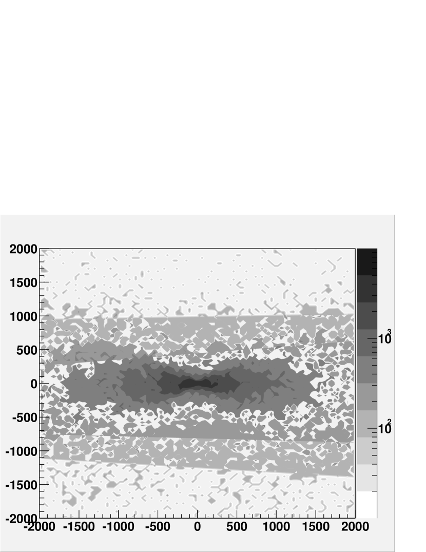
Figure 9: The density of muons in the shower plane. Top panel: MC result, middle panel: CE result, lower panel: CE result with $p_{t}$-kick in source function.

5 CPU times

In ref. [6] it was shown that the CE approach is a factor 20-40 faster than the MC approach, when asking for LDFs of the same statistical quality. A similar enhancement was found in ref. [7] by using the shower library approach.

Of course, it depends very much on the observable to be computed when comparing CPU times. But in general, a typical longitudinal profile without any lateral spread can be computed in about a minute on a 1Ghz CPU. A useful lateral distribution function takes about 10 minutes.

6 Conclusions

Hybrid calculations allow one to reduce considerably the computation time for air shower simulations. The natural fluctuations arise from the first few interactions in the atmosphere and are computed in traditional Monte-Carlo method. Below a given threshold, particles are then replaced with sub-showers taken from a shower library or by the solution of cascade equations. The CE can be solved down to lowest energies, if corrections are applied to account for the neglected lateral expansion. The precise lateral spread can be computed again by MC method, with low energy particles created from the source function.

The hybrid approach, i.e. the combination of traditional Monte-Carlo with efficient numerical methods provides a powerful tool for studying ultra-high energy cosmic rays.

References

- [1] M.Hillas, Proc. 19th Int. Cosmic Ray Conf, La Jolla, USA (1985) 155.
- [2] L.G. Dedenko, Can. J. Phys. 46 (1968) 178.
- [3] L.G. Dedenko, these proceedings.
- [4] K.Werner et al., Invited talk at 9th Hadron Physics and 8th Relativistic Aspects of Nuclear Physics (HADRON-RANP 2004): A Joint Meeting on QCD and QGP, Angra dos Reis, Rio de Janeiro, Brazil, 28 Mar - 3 Apr 2004; T.Pierog et al., these proceedings.
- [5] G. Bossard et al., Phys. Rev. D63, 054030 (2001).
- [6] H. J. Drescher and G. R. Farrar, Phys. Rev. D 67, 116001 (2003).
- [7] J. Alvarez-Muniz, et al., Phys. Rev. D 66 (2002) 033011.
- [8] A. A. Lagutin, et al., Nucl. Phys. Proc. Suppl. 75A (1999) 290.
- [9] D. Heck, J. Knapp, J.N. Capdevielle, G. Schatz and T. Thouw, Report FZKA 6019 (1998), Forschungszentrum Karlsruhe.
- [10] N.N. Kalmykov, S.S. Ostapchenko and A.I. Pavlov, Nucl. Phys. B (Proc. Suppl.) 52B, 17, (1997).
- [11] R. Engel, T. K. Gaisser, T. Stanev and P. Lipari, Prepared for 26th International Cosmic Ray Conference (ICRC 99), Salt Lake City, Utah, 17-25 Aug 1999.
- [12] T. Pierog, H. J. Drescher, F. Liu, S. Ostaptchenko and K. Werner, Nucl. Phys. A 715 (2003) 895.