The DEEP Groth Strip Galaxy Redshift Survey. III.
Redshift Catalog and Properties of Galaxies

Abstract

The Deep Extragalactic Evolutionary Probe (DEEP) is a series of spectroscopic surveys of faint galaxies, targeted at understanding the properties and clustering of galaxies at redshifts $z\sim 1$. We present the redshift catalog of the DEEP 1 Groth Strip pilot phase of this project, a Keck/LRIS survey of faint galaxies in the Groth Survey Strip imaged with HST WFPC2. The redshift catalog and data, including reduced spectra, are made publicly available through a Web-accessible database. The catalog contains 658 secure galaxy redshifts with a median $z=0.65$. The distribution of these galaxies shows large-scale structure walls to $z\sim 1$. We find a bimodal distribution in the galaxy color-magnitude diagram which persists to the same distance. A similar color division has been seen locally by the SDSS survey and to $z\sim 1$ by the COMBO-17 survey. The HST imaging allows us to measure structural properties of the galaxies, and we find that the color division corresponds generally to a structural division. Most red galaxies, $\sim 75\%$, are centrally concentrated, with a red bulge or spheroidal stellar component, while blue galaxies usually have exponential profiles. However, there are two subclasses of red galaxies that are not bulge-dominated: edge-on disks and a second category which we term diffuse red galaxies (DIFRGs). Comparison to a local sample drawn from the RC3 suggests that distant edge-on disks are similar in appearance and frequency to those at low redshift, but analogs of DIFRGs are rare among local red galaxies. DIFRGs have significant emission lines, indicating that they are reddened mainly by dust rather than age. The DIFRGs in our sample are all at $z>0.64$, suggesting that DIFRGs are more prevalent at high redshifts; they may be related to the dusty or irregular extremely red objects beyond $z>1.2$ that have been found in deep $K$-selected surveys. We measure the color evolution of both red and blue galaxies by comparing our $U-B$ colors to those from the RC3. For red galaxies, we find a reddening of only 0.11 mag from $z\sim 0.8$ to now, about half the color evolution measured by COMBO-17. Larger, more carefully defined samples with better colors are needed to improve this measurement. Reconciling evolution in color, luminosity, mass, morphology, and star-formation rates will be an active topic of future research.

1. Introduction

Redshift surveys of the distant universe enable the study of the properties of galaxies at an earlier age, in situ. Large nearby galaxy surveys such as the 2dF Galaxy Redshift Survey (Colless et al. 2001) and Sloan Digital Sky Survey (Abajazian et al.  2003) are now completing the collection of huge samples to determine the structural and stellar-population parameters of local galaxies to high accuracy. At the same time, the development of more powerful multi-object spectrographs on large telescopes is allowing high-redshift surveys to collect truly large samples of distant galaxies, with numbers and detail useful for comparison to the nearby surveys.

The DEEP Extragalactic Evolutionary Probe (DEEP) is a series of large-scale galaxy redshift surveys aimed at studying the evolution of galaxies and large-scale structure to redshifts $z\sim 1$, roughly half the present age of the Universe. The DEEP program is in two parts. The second part, DEEP2, is a large survey of $\sim$65,000 galaxies that is now ongoing with the DEIMOS spectrograph on the Keck 2 telescope. The present paper reports results from DEEP1, an earlier, smaller pilot program using the Low Resolution Imaging Spectrograph (LRIS) on Keck 1. The data reported here cover a subset of the HST Groth Survey Strip (GSS), a mosaic of 28 HST WFPC2 pointings covering 127 arcmin² on the sky in the $V_{606}$ and $I_{814}$ filters (Groth et al.  1994; Rhodes, Refregier & Groth 2000). HST photometry of the GSS reaches to a depth of $\hbox{$V_{606}$}=26$ and $\hbox{$I_{814}$}=25$ (5$\sigma$). The construction of the spectroscopic sample is discussed in Paper I (Vogt et al.  2004 in preparation), and the measurement of photometric structural parameters is discussed in Paper II (Simard et al.  2002).

We present a catalog containing 658 galaxy redshifts, with median $z=0.651$, including 620 galaxies from our spectroscopy and 38 galaxies from other sources (including 33 from the Canada-France Redshift Survey, Lilly et al.  1995a). Galaxies were selected generally to $(V+I)/2=24$ mag (Vega). We use this catalog to discuss the properties of galaxies and large-scale structure to $z\sim 1$, with particular focus on the bimodal distribution of properties of the distant galaxy population.

This bimodality has been discovered recently for local galaxies in Sloan Digital Sky Survey data (e.g., Strateva et al.  2001, Hogg et al.  2003, Kauffmann et al.  2003) and for distant galaxies to $z\sim 1$ in the COMBO-17 photometric redshift survey (Bell et al.  2003a, hereafter B03). Among local galaxies, bimodality is evidenced by a fairly rapid change in galaxy properties near a stellar mass of $3\times 10^{10}$ M_⊙ (Kauffmann et al.  2003). Above that mass, galaxies are generally red with large spheroids; below that, they are blue and disk-dominated.

An easy way to visualize the bimodality is in the color-magnitude diagram, which shows two separate color sequences, a broad blue sequence and a narrower red sequence offset to brighter magnitudes and higher masses. This is shown well, as a function of redshift, by B03. We confirm their finding of a persistent bimodal distribution here and use the particular features of our data to further investigate the properties of both red and blue galaxies.

1.1. Previous redshift surveys

Two published redshift surveys that are comparable in size and depth to DEEP1/GSS are the Canada-France Redshift Survey (CFRS, Lilly et al.  1995a) and the Caltech Faint Galaxy Redshift Survey (CFGRS, Cohen et al.  2000). The CFRS is a magnitude-limited survey to $I_{AB}=22.5$ containing 591 galaxy redshifts with median $z=0.56$ (Crampton et al.  1995). CFRS is roughly 1.5 mag shallower than the nominal limit of DEEP1, but the median redshifts are similar due to differences in the detailed sampling of the magnitude range and to difficulties in obtaining redshifts beyond $z\sim 1.1$ (see Section 3.2). The CFRS is in several fields, one overlapping the Groth Strip. The spectral resolution is 40 Å; a subsample of 246 objects have HST imaging, all with $I$ and many also with $B$ or $V$ (Brinchmann et al.  1998).

The major region surveyed by the CFGRS is the HST Hubble Deep Field, where 602 galaxy redshifts are compiled to $R=24$ in the HDF and $R=23$ in the Flanking Fields (Cohen et al.  2000). The CFGRS combines redshifts from several authors; most spectra were taken using the LRIS spectrograph (Oke et al.  1995), the same instrument used for DEEP1. The typical spectral resolution is 10 Å, and the median redshift is about 0.7. Most galaxies have HST imaging, roughly one quarter being imaged deeply with multiple filters in the HDF, and three quarters imaged lightly in $I$ in the Flanking Fields.

A third survey to which we will make repeated reference is the COMBO-17 photometric redshift survey, in four fields (Wolf et al.  2003; B03). Unlike traditional spectroscopic surveys, this program used intermediate-band photometry in 17 filters to measure restframe colors and redshifts accurate to $\Delta z\sim 0.05$ for 25,000 galaxies from $z=0.2-1$. Recent papers have presented morphological results based on HST ACS imaging of one of these fields, called GEMS (Rix et al.  2004).

1.2. The DEEP GSS Survey

The DEEP1 Groth Strip data have three distinguishing features compared to previous efforts. The spectral resolution is significantly higher, 2.9 Å (FWHM) in the blue and 4.2 Å in the red, yielding a typical velocity resolution of 160 $\rm{km}~{}\rm s^{-1}$. This is high enough for unambiguous identification of the [O ii] 3727 doublet and to permit kinematic linewidth and rotation measurements, which will be presented in separate papers (Weiner et al.  in preparation, Vogt et al.  in preparation). The second feature is HST imaging in both $V$ and $I$ filters, enabling measurement of uniform restframe colors and structural parameters for nearly all objects. The third feature is a single, nearly continuous field with long dimension 40′ on the sky, or 38 comoving Mpc at $z=1$. These features, particularly the HST imaging, are central to our discussion.

Several papers related to the DEEP1 GSS survey have already been published. Koo et al.  (1996) presented a small number of early redshifts. Vogt et al.  (1996, 1997) presented the Tully-Fisher relation for a few resolved disk galaxies. Simard et al.  (1999) measured the evolution of the size-luminosity relation, and Simard et al.  (2002) measured the photometry and structural parameters used in this paper. Of particular relevance is Im et al.  (2002), who identified normal E/S0 galaxies to $I<22$ in the present redshift sample and observed that they populate a narrow color sequence in observed $V-I$ versus redshift. This was used to estimate photometric redshifts for a larger number of E/S0 galaxies without spectra, from which the luminosity function of early-type galaxies was computed. We confirm the narrow range in color of early-type galaxies here and extend the morphological conclusions of Im et al.  (2001) to fainter galaxies.

All HST Johnson-Cousins magnitudes used in this paper are on the Vega system. We use a $\Lambda$CDM cosmogony with $h=0.7,\Omega_{M}=0.3$, and $\Omega_{\Lambda}=0.7$.

2. Observations

2.1. Sample

A series of spectroscopic samples was selected from a photometric catalog produced from HST $V_{606}$ and $I_{814}$ imaging, as described in Paper I (Vogt et al.  2004 in preparation). The limiting magnitude for most objects was $(V+I)/2=24$, based on $1\arcsec.5$ diameter aperture magnitudes. The different samples were designed to explore a range of scientific programs. In addition to a general magnitude limited sample, several types of objects were prioritized for selection from the photometric catalog. These included: elongated candidates for spatially resolved velocity profile extraction, morphologically peculiar objects, extremely blue or red galaxies ($V-I<0.5$ or $V-I>1.75$), and objects with photometric redshifts larger than $z=2$. In addition to the primary targeted objects, we acquired and extracted spectra for objects which fell serendipitously within the slit, and stars placed on slitmasks purely for use in aligning the mask on the sky.

The set of spectroscopic targets is therefore not a strictly random sampling of the photometric catalog. In practice, however, the observed objects sample the range of apparent color and magnitude in the photometric catalog fairly evenly in the range $(V+I)/2\leq 24$ (Paper I, Vogt et al.  2004 in preparation). Combining all objects placed within slits and the objects used for alignment purposes, usable spectra were obtained for a total of 813 different objects.

2.2. Mask design

The spectra were taken with the LRIS spectrograph (Oke et al.  1995) at the Keck telescopes in successive spring seasons from 1995 through 1999. Observations were spread over nine observing runs and 25 nights, in conjunction with several other spring fields. In total, 36 slitmasks were observed in the GSS, where each mask contained typically 30 to 50 slits and several alignment stars.

The first set of ten masks was populated with targets by using printed images of the target fields and transparent overlays, while the rest were designed using interactive, computerized selection; see Vogt et al.  (2004, in preparation). The number of objects per mask increased with time, as we determined the minimum slit length to obtain high quality background-subtracted spectra for objects of a given magnitude and color. Following target and alignment star selection, all masks were modeled with the ucsclris IRAF package written by A.C. Phillips to account for specific observational constraints (e.g., anamorphic corrections) and to create instructions for milling the mask. Nearly all masks were milled with slits of width $1^{\prime\prime}$, with a slit length ranging from $8^{\prime\prime}$ to $12^{\prime\prime}$. After the first year, a small fraction of all slits was tilted at an angle (between $0^{\circ}$ and $30^{\circ}$) relative to the position angle of the mask, in order to trace along the major axis of a spatially elongated object or to capture two objects within one slit.

Certain objects, typically those at magnitudes $(V+I)/2>23$; those with extremely red colors; those for which a redshift could not be determined after initial observations; and spatially extended objects requiring higher S/N, were placed on one, three, or (rarely) more additional slitmasks to obtain more exposure time.

2.3. Observations

Each mask was observed in turn with a blue (typically 900 l mm^-1/5500 Å) and a red (600 l mm^-1/7500 Å) grating, for a combined spectrum covering the range 5000 Å to 8200 Å. We obtained a baseline of $2\times 1500$ seconds exposure per grating per mask, and were able to keep the airmass below 1.3. The spectral resolutions, measured by fitting multiple night sky OH lines in reduced, combined and extracted spectra, are $\sigma=1.25$ Å in the blue spectra and 1.8 Å in the red spectra, or FWHM = 2.9 and 4.2 Å respectively.

A matched flat fielding procedure was developed for the later data. At the end of the night, the telescope was slewed to the same position and the spectrograph rotated to the same position angle as used for the nighttime data exposure. The grating tilt was iteratively adjusted to place a given wavelength at the same pixel as in the nighttime exposure, and then the flat field image was taken. This procedure reduced the effect of CCD fringing and improved the sky subtraction and data quality in the red portion of the spectrum, beyond 7000 Å.

2.4. Data Reduction

Two programs, each crafted for 2-D multislit spectral reductions, were used to reduce these data. Early masks were reduced using Dan Kelson’s Expector software (Kelson et al.  2000). Later masks were reduced using the IRAF Redux package written by one of the authors [ACP]. A few masks were reduced using both of these packages, yielding comparable results.

Both sets of software perform the same group of operations: bias subtraction and trimming of overscan region; “cosmic ray” removal; bad pixel replacement; flat fielding; removal of distortion in the spatial direction; linearization in wavelength; and correction for a “slit function” (removal of the effects of non-uniform slit width).

The primary difference between them is the manner in which calibrations (slitlet location, wavelength) are determined. Expector requires the user to locate slit edges, but automates wavelength calibration, using a cross-correlation algorithm. A wavelength calibration is produced for each spatial position along each individual slitlet, using night sky lines and, if necessary, arc spectra in the blue, taken through each mask.

Redux performs its calibrations in a very different way. The program uses an optical model of the spectrograph consisting of three parts: (1) a mapping of mask location to grating input angles; (2) a transform into and out of the grating coordinate system, where the grating equation is used to describe the dispersion and line-curvature; and (3) a mapping of grating output angles to the detector. This reduces the effective unknowns to two for each mask: an error in the grating tilt and an error in the grating “pitch.” (A third grating variable, the rotation about the grating normal, is solved using arc spectra taken through a special mask and is assumed constant for a given observing run.) The software uses the model and the mask design to predict location of slit edges and bright night sky lines; the offset in the slit locations and the night sky lines then provide the solution for the two unknown variables. The grating tilt error is calculated for each individual slitlet to provide more precise zero-points in wavelength. The location of each slitlet and the wavelength solution within each slitlet are then known to quite good precision for the entire image.

Both Expector and Redux have advantages and shortcomings. Expector performs empirical calibrations for each mask using spectra taken through that mask, but when arcs are used the significant flexure in LRIS means that the calibrations may not be as accurate for the science data, and offsets must be added. In addition, sparse regions in the arc spectra (typical in the blue) cause uncertainties in the wavelength solution. Redux, on the other hand, is limited by the precision of the optical model. Using combined data sets with a variety of gratings and spanning large ranges in grating tilt, typical rms errors are $\sim$0.6 px (0.13 arcsec spatially; in dispersion, 0.51 Å and 0.77 Å in the blue and red, respectively), and the errors are rarely worse than $\sim$1–1.5 px in the very corners of the image. For most science spectra, the results are better than this, particularly as the wavelength scale is zero-pointed using night sky lines.

Fringing in the red has always been a difficult problem due to the strong night-sky lines in the OH “forest”. Given the flexure in LRIS, it was often found that applying a “fringe frame” correction exacerbated the problem rather than reducing it. Thus, in the earlier data, fringe frames were only employed if they improved night-sky subtraction. This problem was solved in later data by taking red flat-fields at the end of the night, matched in wavelength to the science image as described above. In these data, fringe frame corrections were always applied and always produced good results.

Individually-reduced 2-D linearized and rectified spectral images for each object were collected for all observing runs and combined using a biweight estimator, resulting in two final combined 2-D images, one each for the red and blue gratings. One-dimensional spectra were then extracted from these combined images, with a minimum object width of 1.5 arcseconds.

3. Redshift Catalog

3.1. Redshift Determination

We inspected the 1-D and 2-D spectra by eye to find spectral features. For all candidate redshifts, we verified the existence of features by visual inspection and assigned a quality code. For galaxies at $0<z<1.4$, the primary features are nebular emission lines, principally [O ii] 3726 3729, H$\beta$ 4861, [O iii] 4959 5007, and H$\alpha$ 6563; for absorption-line objects the strongest features are Ca II H+K 3933 3969, the CH G-band at 4304 Å, Balmer lines, and the 4000 Å break. Some high-$z$ objects are identified by interstellar absorption lines of Mg II 2796 2803 and Fe II 2586 2600. Cool, late type stars are generally identified by absorption bands; hotter stars often have featureless spectra in our wavelength region and are more difficult to identify.

We consider a redshift secure if at least two features are detected. Since the spectral resolution is high, many galaxies have clearly resolved [O ii] doublet emission, which is counted as two features. Objects with a secure redshift from two or more features are given a redshift quality A in column 5 of Table 1.

Some galaxies have a broad emission line consistent with the [O ii] doublet separation of 220 $\rm{km}~{}\rm s^{-1}$, but not resolved into two components. These galaxies have an almost certain redshift, since the appearance of broad [O ii] in the 2-D spectra is distinctive, and there is generally no other convincing candidate for the emission line. These and other objects with a nearly certain redshift but without two strong distinct features are “almost secure” and are given a quality B in column 5 of Table 1.

All redshifts were checked by at least two people (Phillips, Sarajedini, Koo, Weiner) and disagreements on redshift and quality were resolved. Final redshift qualities were systematized by one of us (BJW) to assure uniformity. We estimate that quality A have $>99\%$ confidence and quality B have $>90\%$ confidence. Our analysis of the galaxy sample below uses both the quality A and B objects.

A few objects have a single feature, very weak features, or other spectral properties which suggest a redshift, but the redshift is by no means certain. We do not count these as identified or use these objects in the analysis of galaxy properties below. The uncertain redshifts are not listed in Table 1 but can be retrieved from our Web database. There are very few objects with a single strong spectral feature that yields an ambiguous redshift.

Objects for which a redshift, 136 in total, could not be determined with confidence are coded with quality F in column 5 of Table 1. These include objects with low signal-to-noise and objects with fairly high S/N but no identifiable features. A small number of objects, $\sim 20$, fell off the slit, off the detector, or had otherwise unusable data; these objects are not listed in Table 1 and are not counted in our completeness statistics.

Table 1Redshift catalog for the DEEP 1 Groth Strip Survey

Note. — The complete version of this table is in the electronic edition of the Journal. The printed edition contains only a sample.

The high resolution of the LRIS spectra allowed us to determine redshifts to a few parts in $10^{-4}$. We quantified redshift accuracy by comparing to observations of the Groth Strip from the ongoing DEEP 2 survey with the DEIMOS spectrograph, at even higher spectral resolution. The DEEP2 redshifts are known to be accurate to 30 $\rm{km}~{}\rm s^{-1}$. From 140 galaxies with both DEEP1 and DEEP2 redshifts, we find an offset of (DEEP1-DEEP2) $=9$ $\rm{km}~{}\rm s^{-1}$ and an RMS $=51$ $\rm{km}~{}\rm s^{-1}$. The RMS error of DEEP1 redshifts is thus $\sigma_{V}=42$ $\rm{km}~{}\rm s^{-1}$; in redshift it is $\sigma_{z}=2.3\times 10^{-4}$, with a possible but small systematic offset.

A portion of the redshift catalog is shown in Table 1. The table contains an entry for every object for which a usable spectrum was actually obtained, including alignment stars but not including objects that fell off the slit or where the data were completely unusable. 47 objects with redshifts from non-DEEP sources (Lilly et al.  1995a; Brinchmann et al.  1998; Hopkins et al.  2000)are listed at the end of the table. Only the first page of the table is reproduced in the printed journal. The full table is available in the electronic version, and the catalog and data, including extracted spectra, are publicly available through a World Wide Web interface at http://saci.ucolick.org.

41 objects with redshifts fall on or near the edges of the area imaged with HST, or next to bright objects, and their total magnitudes and structural parameters could not be measured with gim2d. These do not have $V$ or $I$ magnitudes listed in Table 1, although for 31 we were able to compute aperture magnitudes and infer restframe magnitudes. Values which are unmeasured, such as for objects without magnitudes or redshifts, are flagged by clearly out-of-range values, typically -99 or -999.

The columns in Table 1 are:

Column 1. Object ID, referring to WFPC2 chip number and pixel position; see Paper I.

Columns 2-3. RA and Dec, epoch J2000.

Column 4. Redshift. Redshifts noted “a” are from the CFRS (Lilly et al.  1995a), “b” are from Brinchmann et al.  (1998), and “c” are from Hopkins et al.  (2000).

Column 5. Redshift quality. “A” is a secure redshift based on two or more spectral features. “B” is an almost-secure redshift based on one feature such as a broad line that is almost certainly [O ii] 3727. “F” indicates a failure to obtain a redshift. “A” and “B” are secure enough to be used in the analysis in the remainder of this paper.

Column 6. Redshift source: 1=CFRS (Lilly et al.  1995a), 2=Brinchmann et al.  (1998), 3=Hopkins et al.  (2000), 4=DEEP.

Column 7-8. Exposure times for red and blue spectra.

Column 9. Total $I_{814}$ magnitude from structural models fit to the $I$ image using gim2d by Simard et al.  (2002).

Column 10. $V_{606}-I_{814}$ color. $I_{814}$ is from Column 9; $V_{606}$ is the analogous magnitude fitted to the $V$ image. For most (602) objects, the “simultaneous” fit quantities from Simard et al.  (2002) are used, in which $V$ and $I$ fits are constrained to have the same size parameters. For 13 objects, these are unavailable, and the “independent” fits are used.

Column 11. Absolute magnitude $M_{B}$ based on apparent magnitude and color using the K-correction procedure described below. For 615 objects, gim2d total apparent magnitudes are used to infer $M_{B}$; for 31 objects, total magnitudes were not available and aperture apparent magnitudes were used.

Column 12. $U-B$ restframe color, derived through the K-correction procedure described below.

Column 13. Half-light radius $R_{hl}$ in arcsec from the structural model fit to the $I_{814}$ image by Simard et al.  (2002). This is the half-light radius of the face-on reconstructed model before PSF convolution. It is more physically meaningful than the raw half-light radius in circular apertures and is larger than the latter for edge-on galaxies.

Columns 14 and 15. Bulge-to-total $B/T$ ratio and central concentration $C$ from the $I_{814}$ image by Simard et al.  (2002).

Columns 16 and 17. Equivalent width and wavelength of the strongest emission line.

Column 18 and 19. Morphological type and peculiarity code of red galaxies, as defined in Section 5.4.

Table 2 summarizes the numbers of spectra taken and redshifts identified in the DEEP GSS redshift survey. A small number of additional redshifts are provided by other observations in the Groth Strip, mostly by the CFRS (Lilly et al.  1995a), and these are listed at the end of Table 1 and counted in Table 2. They are excluded from the following discussion of completeness.

Table 2Redshift statistics for the Groth Survey Strip

		Quality
	total	A	B	No $z$
DEEP total	813	619	52	142
Galaxies	620	572	48	-
Stars	51	47	4	-
No redshift ID	142	-	-	142
CFRS+others	47	36	11	-
Galaxies	38	28	10	-
Stars	9	8	1	-
DEEP+CFRS+others
Galaxies	658	600	58	-
Stars	60	55	5	-

Figure 1 shows the final DEEP1/GSS galaxy redshift histogram, including 620 DEEP redshifts and 38 redshifts from other sources. The median $z$ is 0.651, and the number of galaxies drops off rapidly above $z=1.05$. This decline is probably due to the redshifting of [O II] 3727 into the bright atmospheric OH band at 7700 Å, where it can be masked by poor sky subtraction. The redshift completeness is discussed in the next section. A few objects are identified at very high redshift by their UV interstellar absorption lines or broad AGN emission. One object at $z=3.40$ is the source in the quadruple gravitational lens galaxy 093_2470, identified through Ly$\alpha$ emission.

Figure 1.— Redshift histogram including quality A+B redshifts for the GSS sample, including DEEP1 and other sources. Sharp spikes indicate large-scale structure features permeating the volume. The sharp decline in the number of galaxies near $z\sim 1.05$ coincides with the movement of [O II] 3727 into the bright atmospheric OH band at 7700 Å.

3.2. Completeness

The completeness of the DEEP1 spectroscopic survey is defined as the fraction of observed targets successfully identified as galaxies or stars with quality A or B. Here, observed targets include all objects for which a usable spectrum was extracted, including alignment stars but not including those objects that fell off the slit, off the edge of the CCD, or were otherwise corrupted. Since there was zero possibility to obtain redshifts for these, it is as if they had never been observed. In this section, we discuss only DEEP1 targets and omit redshifts from other surveys.

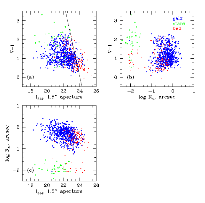
Figure 2.— Redshift success versus apparent magnitude, color, and half-light radius for all spectroscopic targets. Blue filled circles = galaxies, green open circles = stars, red triangle = no redshift. The nominal selection limit of the survey, $(V+I)/2>24$, is shown by the diagonal line in panel (a). Objects with failed $z$’s are more frequently faint, blue, and small, but most are not stars, which are pointlike. Followup spectroscopy by DEEP2 and other surveys shows that most faint blue objects lie beyond the useful range of the present survey, namely $z\sim 1.05$, where OH interferes with [O II] 3727 (cf. Figure 1).

Figure 2 shows the apparent color-magnitude diagram for galaxies, stars, and targets without redshifts. The most striking feature of this diagram is the concentration of failures at faint magnitudes and very blue colors ($V-I<1$). Such blue galaxies are expected to have strong emission, so it is unlikely that they were missed on account of weak spectral features. We suspect that they simply lie beyond the effective redshift range of the survey, $z\sim 1.05$, set by bright OH at 7650 Å. This is confirmed by subsequent DEEP2 observations, which are taken at higher spectral resolution, are less contaminated by OH emission, and reveal large numbers of galaxies beyond $z=1.05$ out to the DEEP2 redshift limit $z=1.4$; many of these occupy the region where DEEP1 failures lie. Further information on blue redshift failures is provided by measurements probing the “redshift desert” by Steidel et al.  (2004), who show that many galaxies successfully recovered in the range $z=1.5-2.5$ display colors similar to the blue failures here. Some of these are actual followup observations of DEEP2 failures by that group, showing most of them to lie beyond $z=1.4$. In totality, this information is powerful evidence that the bulk of blue redshift failures in DEEP1 lie beyond $z=1.05$.

The situation is different for red failures with $V-I>1.5$, which tend to lie further above the nominal survey magnitude limit, as seen in Figure 2. At $22.5<(V+I)/2<23.5$, the failure rate is higher for red objects than for blue objects. This is plausible because it is harder to identify a redshift for faint red objects with weak or no emission lines.

Figure 3.— The dependence of redshift success on $(V+I)/2$, by number (top) and by fraction (bottom, success: solid, no redshift: dashed). The half-power success point is $(V+I)/2=24$, which may be taken as the effective magnitude limit of the survey.

Figures 3 and 4 quantify the information in Figure 2. Figure 3 plots the number and fraction of targets and quality A+B identified objects as a function of $(V+I)/2$ magnitude. The completeness fraction declines only slowly with magnitude, remaining at 80% at $(V+I)/2=23$, but drops to 50% in the $(V+I)/2=24$ bin. Only a few objects are identified at $(V+I)/2>24$. Thus the limiting magnitude of the survey is effectively $(V+I)/2=24$.

Figure 4.— The dependence of redshift success on $V-I$ color, by number (top) and by fraction (bottom, success: solid, no redshift: dashed). Figures 2 and 3 combined with this one show that redshift failures are primarily blue and faint. Additional spectroscopy indicates that most of these are objects beyond our effective redshift limit $z\sim 1.05$.

Figure 4 plots the completeness fraction against color. Incompleteness increases strongly for galaxies bluer than $V-I=1.0$, and for the bluest objects, it is very high. As noted, we believe these objects to be at $z\gtrsim 1.05$.

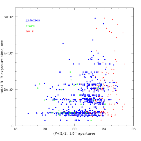
Figure 5.— Redshift success in $(V+I)/2$ magnitude and exposure time space. The total exposure time (blue+red wavelength settings) versus $I$ magnitude, with points coded for galaxies = blue circles, stars = green open circles, and no redshift identified = red triangles.

Figure 5 shows the distribution of targets in magnitude and exposure time with points coded as confirmed galaxies, confirmed stars, or no redshift. This figure suggests that increased exposure time on the faintest objects produces only a marginal improvement in the success rate. This is again understandable if most of the failed objects are are outside the effective wavelength range. This argument applies to the blue galaxies, but one would expect that red failures might yield more frequently to longer exposure times. Unfortunately, the distribution of exposure times for red galaxies does not permit a test of this.

Figure 2 provides additional information on the apparent sizes of objects. In other redshift surveys, with objects selected from ground-based images, the separation between stars and galaxies is sometimes blurry. The excellent resolution of HST for all objects here removes that problem, and Figure 2 shows a clean separation between pointlike objects and resolved galaxies. The separation is especially clean because the HST PSF is accounted for.

Of pointlike objects with redshifts, only two prove to be non-stellar: a QSO and a subcomponent of an interacting galaxy. Thus, most of the pointlike objects without successful redshifts are presumably stars. Most stars at these faint magnitudes are cool dwarfs with broad absorption bands, or hotter stars with nearly featureless spectra, occasionally showing H$\alpha$ or Ca II absorption. We are generally able to positively identify red, cool stars with $I\lesssim 22$ from their absorption bands. Fainter than $I=22$, the continuum is too weak to make positive identifications. The hotter stars are more difficult since their spectra have few or no features. Figure 2 shows a number of unidentified pointlike objects with $0.5<V-I<1.5$ that are presumably hot stars. There appears to be no substantial population of intrinsically small, pointlike field galaxies. Surveys which weed out pointlike objects will miss QSOs, but will not miss a significant number of galaxies if their star/galaxy separation is good.

4. Galaxy colors

Restframe colors and magnitudes are essential to study the evolution of galaxy properties. For galaxies with redshifts, observed HST $V_{606}-I_{814}$ color from Table 1 is used to infer both restframe $U-B$ color and K-correction ($K_{IB}$) from observed $I$ to rest $M_{B}$. To obtain K-corrections and restframe colors, we use a set of 34 galaxy UV-optical spectral energy distributions selected from the atlases of Calzetti et al.  (1994) and Kinney et al.  (1996). The SEDs are those of ellipticals, spirals, and starbusts with continuous wavelength coverage; a few abnormal spectra were excluded.

The first step in the K-correction is to synthesize a restframe $U-B$ color for each of the atlas SEDs using the system response curves for each filter and the zeropoints of the UB Vega system (Fukugita et al.  1995). Next, for each DEEP galaxy we redshift each atlas SED to the redshift of the galaxy and convolve the $f_{\lambda}$ SEDs with the response curves to synthesize an observed HST $V-I$ color and K-correction $K_{IB}$ from observed $I$ to restframe $M_{B}$. We then fit low-order polynomials to the resultant atlas $U-B$ and $K_{IB}$ values as a function of synthesized $V-I$. Entering these fits with the observed $V-I$ color of the DEEP1 galaxy yields $K_{IB}$ and $U-B$. A few very blue galaxies are bluer than any of the SEDs and are truncated to $U-B=-0.6$ to avoid extrapolation. The procedure is described further in Willmer et al.  (2004, in preparation) and is similar to that used in Gebhardt et al.  (2003) except that here we fit a polynomial over $V-I$ at each galaxy redshift rather than over $V-I$ and $z$ simultaneously. The resultant values of $U-B$ and $M_{B}$ are given in Table 1.

Error estimates in restframe $U-B$ prove to be important, especially for red galaxies. The error from photon statistics in raw $V-I$ is relatively small. The Monte Carlo error estimation of Simard et al.  (2002) models photon statistics and errors from the photometric model fits, yielding median errors in $V-I$ of 0.055 mag for this sample. We have also compared the model colors to aperture colors measured through a 1.5″ aperture, and find that the rms scatter between the two colors is only 0.085 mag, which is consistent. The transformation from $V-I$ to $U-B$ mutiplies the apparent color error by a factor dependent on redshift, from $\sim 1.0$ at $z\sim 0.3$ to 0.6 at $z\sim 0.9$, yielding net random errors in $U-B$ of 0.03-0.04 mag from $z=0.4$ to 1.0.

The remaining sources of error are systematic errors in the transformation from $V-I$ to $U-B$. At $z=0.8$, the $V$ and $I$ bandpasses correspond very closely to restframe $U$ and $B$, and the color K-correction is small. At redshifts other than $z=0.8$, the color does not translate so closely, but our K-correction procedure yields accurate restframe colors for $0.4<z<1.2$; nearer than that, the correction is less reliable. We have checked that the procedure introduces minimal scatter using methods to be explained in Section 5.9, but it is possible that there are still small zeropoint shifts as a function of redshift. We also have completely independent ground-based photometry for all galaxies from the Canada-France-Hawaii Telescope in $B$, $R$, and $I$ filters (Kaiser et al.  in preparation), and have used these to compute an independent restframe $U-B$ color. For galaxies at $z>0.4$, the CFHT-derived $U-B$ values agree well with the present ones with an rms scatter of 0.12 mag and a zeropoint offset of 0.02 mag, the HST colors being redder.

A final source of systematic error is the difference between colors from an energy-weighted convolution of the $f_{\lambda}$ SED with the response curve, as described above, and from a photon-weighted convolution. In principle, since no color term was applied to the HST magnitude solution (Simard et al.  2002), the photon-weighted convolution is correct when the HST zeropoints are determined for an object the color of Vega. In practice, photon-weighting makes the inferred $U-B$ colors redder, but the difference is only a mean of 0.02 mag and RMS of 0.014 mag, and we have not applied this offset to the tabulated values. To sum up, we believe that the typical random error of $U-B$ is 0.03-0.04 mag in the critical redshift range $0.4<z<1.0$, with systematic errors in zeropoint at $z=0.8$ of $\sim 0.02-0.03$ mag.

5. Results

5.1. Redshift Distribution

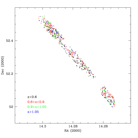
Figure 6.— Distribution of DEEP 1 GSS galaxies on the sky. Galaxies are color coded by redshift range: black: $z<0.6$; red:$0.6<z<0.9$; green:$0.9<z<1.05$; blue:$z>1.05$.

The distribution on the sky of DEEP1/GSS galaxies with redshifts is shown in Figure 6. The spectroscopy samples an area approximately 3′ $\times$ 40′. Here and subsequently, we include the 38 galaxy redshifts from sources outside DEEP1, located primarily at the northeast end of the Groth Strip. Some areas of the Groth Strip are more densely covered than others, and there are patches without any coverage at all. The limited area and non-uniform sampling preclude quantitative statements about the 3-D galaxy distribution or local galaxy overdensities. These statistics are much better probed in the ongoing DEEP 2 survey, which has larger area and statistically uniform sampling (e.g., Coil et al.  2003).

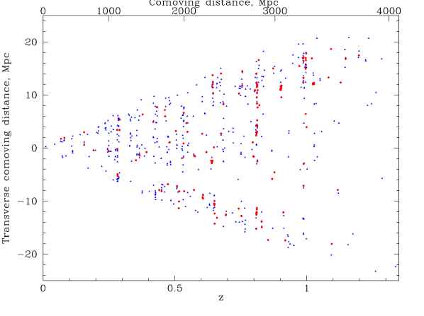
Figure 7.— “Pie” diagram of galaxies in the Groth Strip. The transverse spatial dimension is stretched to show points more clearly. Large-scale structures of voids and walls persist to $z\sim 1$. Blue galaxies are plotted as blue triangles, and red galaxies as red filled circles; red galaxies appear to populate denser regions, as demonstrated quantitatively in the clustering analysis of DEEP2 data by Coil et al.  (2003).

The “pie diagram” in Figure 7 plots transverse distance of each galaxy in comoving Mpc along the slice versus redshift. “Walls” and filaments due to large-scale structure cross the volume, with the most prominent ones at $z=0.28,0.81,0.99$. The transverse distance is stretched to enhance the visibility of points in dense regions.

Galaxies in the $z=0.99$ wall stretch over 37 comoving Mpc, demonstrating that large-scale structure is already prominent at $z\sim 1$. The $z=0.99$ feature was already noted as a redshift peak in the CFRS survey by Le Fèvre et al.  (1994, 1996) and in early DEEP1 data by Koo et al.  (1996). Filamentary/wall structures on this and even larger scales are prominent in local surveys, as shown in the Las Campanas Redshift Survey (Doroshkevich et al.  1996), the 2dF Survey (Colless et al.  2001), and the SDSS Survey (Zehavi et al.  2002), and strong redshift peaks were noted in early high-$z$ field galaxy redshift surveys and ascribed to large-scale structure (e.g., Broadhurst et al.  1990; Willmer et al.  1994; Le Févre et al.  1994; Cohen et al.  1996; Connolly et al.  1996).

It is therefore no surprise, given our knowledge of how structure forms and the nature of galaxy biasing, to find large, well developed structures already outlined by galaxies at $z\sim 1$. Figure 7 is one of the first cuts through the Universe to show a full 2-D view of this structure to high redshift, other ones being early DEEP2 data by Coil et al.  (2003) and early VIMOS VLT Deep Survey (VVDS) data by Le Fèvre et al.  (2004). The three pictures are qualitatively very similar.

5.2. Color bimodality

Figure 8 gives an overview of magnitudes and colors (both observed and restframe) versus redshift. The most striking feature is the bimodality in restframe $U-B$ (panel d). Galaxies are divided into red and blue populations, and this division persists to $z=1$. The division is at approximately $U-B=0.10$, which has been used to color-code the points in Figures 8 and 7. Figure 9 shows the bimodal distribution of restframe $U-B$ color in DEEP1 and, for comparison, the colors of a local sample from the RC3 (de Vaucouleurs et al.  1991). We expand on this comparison in Section 6.

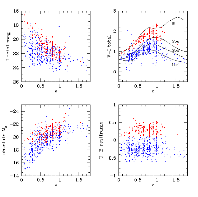
Figure 8.— Galaxy magnitudes and colors versus redshift. Color bimodality is clearly seen in both apparent $V-I$ and restframe $U-B$. Galaxies are plotted as red circles or blue triangles according to whether $U-B$ is greater or less than 0.1. Color tracks of non-evolving local-galaxy SEDs from Coleman, Wu, and Weedman (1980) are shown in the upper right panel. No single CWW track exactly follows the valley between red and blue galaxies.

The existence of restframe color bimodality in GSS data confirms a similar hint noted by Im et al.  (2002) for DEEP1 data based on apparent color, and is consistent with the definitive discovery of color bimodality for distant galaxies by COMBO-17 (B03) based on a much larger sample. The same effect is seen in DEEP2 data using principal component analysis of galaxy spectra (Madgwick et al.  2004). Bimodality has been much discussed for local galaxies by the SDSS collaboration (e.g., Strateva et al.  2001; Blanton et al.  2003; Hogg et al.  2003), and for 2dF data (Madgwick et al.  2002) although it turns out to have been clearly present in RC3 data (de Vaucouleurs et al.  1991) all along (see below and Figure 8 of Takamiya et al.  1995). Roughly speaking, red galaxies are consistent with passive populations and little star-formation, or with dust reddening (see Section 5.8), while blue galaxies are star-forming. A galaxy which stops forming stars will fade and redden across the blue/red divide in a few Gyr. As emphasized by Kauffmann et al.  (2003), bimodality for local galaxies is not restricted to color alone but extends to many other galaxy properties such as luminosity, mass, concentration index, star-formation history, and environment, which are all correlated with color.

Figure 9.— Upper panel: Total restframe $U-B$ color distribution for DEEP 1 galaxies. Lower panel: Total $U-B_{T}$ color distribution for galaxies from the RC3 catalog with $B_{T}^{0}<13.5$.

The existence of color bimodality is thus a fundamental property of the galaxy population, and its presence out to $z\sim 1$ means that it was established fairly early in the evolution of galaxies. An important task is to ascertain whether the other properties that correlate with bimodality locally (such as luminosity, mass, etc.) also do so for distant galaxies. We explore such correlations in the remaining sections of this paper.

In addition to being of theoretical interest, bimodality is of practical significance because it means that distant galaxies can be accurately sorted into groups using an easily measured parameter, color. This is needed because it is obvious that different classes of galaxies have had different evolutionary histories, and it is even possible that some galaxies have evolved from one type into another. Sorting, counting, and tracking by type is thus essential. In previous surveys, this has often been done by dividing galaxies according to the non-evolving SEDs of Coleman, Wu, & Weedman (1980), as illustrated in panel (b) of Figure 8. The Sbc SED, second from the top, has been used to divide red and blue galaxies (as in the CFRS, Lilly et al.  1995b). This SED does not quite follow the valley between red and blue galaxies. Dividing galaxies at this SED can therefore mix the two types; sorting by any non-evolving SED or color can introduce redshift-dependent errors in the counts if the location of the valley evolves. It is safer to have an index of red/blue that evolves along with the galaxy population itself, which color provides, if the sample is large enough. In this paper we will generally divide red and blue at restframe $U-B=0.1$, which is applicable to $0.4<z<1.0$ where the majority of our sample lies, but not in the local universe. Samples with very large numbers such as COMBO-17 (B03) or DEEP2 allow a finer determination of the evolving division.

Interestingly, a division by color for high-redshift galaxies is not seen in CFRS data (Crampton et al.  1995). Possibly the bimodality was washed out by the relatively larger color errors in the CFRS 3″ ground-based aperture ($\sim 0.15$ mag, Le Fèvre et al.  1994). This highlights the desirability of obtaining precise colors in studies of distant galaxy evolution. The CFGRS approached classification for high-redshift galaxies somewhat differently, using spectral typing into 3 classes rather than restframe color; there is a hint of a bimodal distribution in spectral index in Figure 8(a) of Cohen (2001). The CNOC2 survey divided galaxies into 3 classes based on SED types derived from CWW SEDs and fit to the apparent colors, a scheme that is closely related to restframe color (Lin et al.  1999). Their sample from $0.12<z<0.55$ shows a distinct bimodality in SED type, but the 3 galaxy classes were not chosen to follow the bimodality.

5.3. Color-magnitude diagram

Figure 10 shows the restframe color-luminosity diagram of the DEEP1 galaxies. The bimodal division in color also corresponds to a difference in the distribution of luminosities: red galaxies are slightly more luminous in restframe $B$ than the brightest blue galaxies. The distribution in color and magnitude is qualitatively consistent with the distributions seen in the SDSS sample locally (Blanton et al.  2003; Hogg et al.  2003) and with the CM diagrams of B03. Luminosity functions computed by color show a systematic dependence of $L^{*}$ on color for local galaxies, with $L_{B}^{*}$ being more than 1 magnitude brighter for the reddest local galaxies compared to the bluest in SDSS (Blanton et al.  2001). Similar behavior is seen at high redshift in the COMBO-17 sample (Wolf et al.  2003), and in both DEEP1/GSS and early DEEP2 data by Willmer et al.  (2004, in preparation). Figure 10 also codes red galaxies by morphological type, discussed in Section 5.4.

Figure 10 shows the changing effect of the magnitude selection limit $(V+I)/2=24$ as a function of redshift. The near-vertical lines in each panel indicate the selection limit at the median redshift for that bin, $z=0.4$, 0.75, 1.0 respectively. At low redshifts, the selection, which is effectively $R$ band, favors intrinsically red galaxies slightly. At high redshifts, the selection moves to restframe blue or near-UV wavelengths, and intrinsically red galaxies are disfavored. Beyond $z=1.1$, there are few red galaxies in the sample, simply because the steep drop in their luminosity function at $L^{*}$ means few exist which are bright enough to be selected. This effect is also seen in the $M_{B}(z)$ panel of Figure 8.

However, at low redshift, we find few faint red galaxies, even though they are not selected against; measurements of the luminosity function by color are discussed further in Willmer et al.  (2004, in preparation). Some low-redshift field-galaxy surveys find that the luminosity function of red galaxies falls at faint magnitudes (e.g., SDSS, Blanton et al.  2001). Our data appear to agree, though care must be taken in interpreting the LF falloff, since the color-magnitude relation slope for red galaxies means that a division at fixed restframe color can produce a red LF which falls at the faint end.

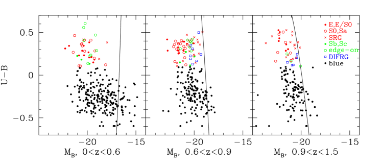
Figure 10.— Restframe color-magnitude diagram for Groth Strip galaxies in three redshift ranges. The dividing line for red galaxies used here is $U-B$ = 0.1. Points for red galaxies are color-coded by morphological type: red filled circle = E; red open circle = E/S0-Sa; red x = small red spheroidal galaxy; green filled circle = Sb-Sc; green open circle = edge-on disk; blue open square = diffuse red galaxy. Galaxies in the blue population (below $U-B=0.1$) are not classified. The magnitude limit of $(V+I)/2=24$ for the median redshift in each bin, $z=0.4,0.75,1.0$, is shown as the near-vertical line in each panel.

The mass difference between red and blue galaxies is minimized in Figure 10 by use of blue magnitude $M_{B}$, which penalizes red galaxies. Figure 11 replots the CM diagram as a function of approximate stellar mass using $M_{B}/L$ values as a function of $B-V$ (transformed to $U-B$) from Bell et al.  (2003c). A downward correction of 0.15 dex has been applied to convert to a Kroupa IMF (Kroupa, Tout, & Gilmore 1993), as advised by Bell et al.  (2003c). The true mass variation with color is now more apparent. By eye, the division between red and blue galaxies occurs at $3\times 10^{10}$ M${}_{\odot},$ the same value found for SDSS galaxies by Kauffmann et al.  (2003). However, the selection against red galaxies at $z\sim 1$ penalizes lower-mass red galaxies, so the lack of red galaxies below $3\times 10^{10}$ M_⊙ is partly a selection effect.

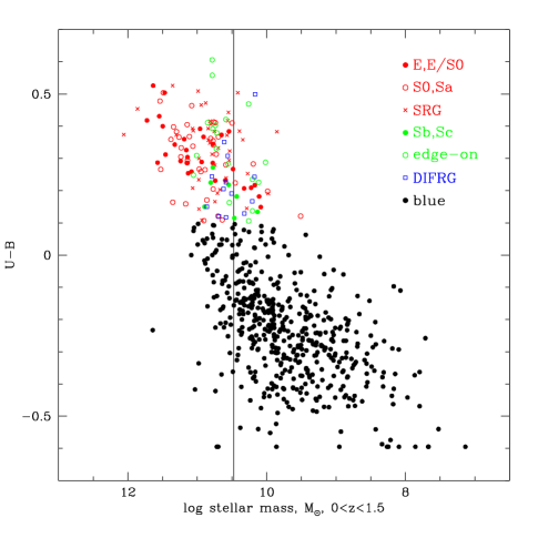
Figure 11.— Restframe color versus approximate stellar mass. Mass is derived from magnitude and color following the prescription of Bell et al.  (2003c). Red galaxies are coded for morphological type as in Figure 10. The vertical line is the break at $3\times 10^{10}M_{\odot}$ in properties of local galaxies found by Kauffmann et al.  (2003). In our sample, red galaxies to the right of this line are potentially lost at high $z$ due to magnitude selection effects.

Though the dividing line between red and blue galaxies is far from sharp in mass, it is a useful generalization that massive galaxies made the bulk of their stars early and have now largely shut down (Im et al.  2002). The existence of color bimodality at $z\sim 1$ indicates that this process had occurred in many massive galaxies by that time. The mechanism that quenched star-formation in the most massive galaxies is not known and is receiving much attention lately (e.g., Benson et al.  2003, Binney 2004, Granato et al.  2004). COMBO-17 (B03) estimate that the total stellar mass in galaxies in the red population has doubled since $z=1$, implying that the quenching of a significant fraction of the red stellar mass has occurred at surprisingly late epochs.

The brightest red galaxies are somewhat more luminous than the brightest blue galaxies, which raises the question of how bright red galaxies are assembled, as observed by Bell et al.  (B03). Since the blue galaxies will fade as they redden, the observed blue galaxies cannot be the progenitors of the red galaxies, unless blue galaxies merge at $z<1$ to build up the most massive red galaxies. The dilemma becomes even more apparent when color is plotted against the stellar masses of galaxies, as in Figure 11. Possible alternatives are that luminous red galaxies are assembled largely before $z=1$, that they are built up in sites of obscured star formation, or that they are assembled by mergers of red and/or blue galaxies. Mergers of red galaxies are favored by B03 on the basis of their measurements of evolution in red galaxy color and luminosity density. Color evolution and the sloping color-magnitude relation for red galaxies will provide a strong constraint on models for red galaxy assembly. The topics of quenching and mass assembly on the red sequence will receive intense scrutiny as surveys like DEEP2 and VVDS gather more data.

5.4. Morphologies of red galaxies

The WFPC2 imaging of the Groth Strip provides enough spatial resolution for a visual, morphological classification of most galaxies in our redshift sample. Although morphology can be subjective, it is valuable for understanding the nature of the red/blue galaxy division and its relation to galaxy structure. The red population at $z=0$ is known to consist largely of early types (E-Sa), while the blue population contains later-type disk galaxies and irregulars (Sb-Irr). This is shown below using RC3 data (Figure 17). The question then arises, what are the morphology and structure of red and blue galaxies at higher redshift? The following discussion focuses on red galaxies; blue galaxies are deferred to a future paper.

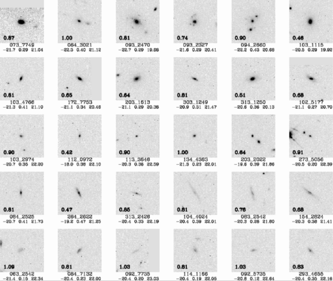
Figure 12.— HST WFPC2 $I_{814}$ images of distant red galaxies illustrating the three major morphological groups. Images are 10 arcsec on a side. The first three rows contain spheroid-dominated red galaxies, or SRGs: the first row shows E types, the second E/S0 through Sa, and the third row shows small spheroidals, which are too small to determine a detailed type. The fourth row shows the second group, edge-on galaxies; detailed Hubble types cannot be assigned to these due to orientation, though some clearly have spheroids. The bottom row shows the third major group, diffuse red galaxies, or DIFRGs. The panels are labeled with galaxy redshift (in panel), GSS ID, $M_{B}$, $U-B$, and $I$ magnitude.

Table 3Morphological types of red galaxies

Type	Code	$z<0.7$	$z>0.7$	Total
E	-5	15	13	28
E/S0, S0, Sa	-3,-2,0,1	24	16	40
Small SRG	30	8	31	39
Sb,Sc	3,5	5	2	7
Edge on disk	50	11	7	18
DIFRG	40	3	11	14
Total		66	80	146

5.4.1 Morphological classification scheme

There are 146 red galaxies with redshifts, defined by $U-B>0.10$. A first look at the sample suggested that a small number of categories could accommodate them. We then classified the red galaxies into the categories listed in Table 3. Nearly all fell into one of three main categories: spheroid-dominated, edge-on disk, and diffuse. These categories were influenced by the appearance of typical spheroid-dominated red-sequence galaxies at $z=0$ as well as the need to identify other classes of objects whose redness may have a different cause. Examples of our classes are shown in Figure 12.

The spheroid-dominated category (hereafter called SRG, for “spheroidal red galaxy”) contains objects from E to Sa. Such objects are presumably red because they are dominated by old stars. Types were assigned to these galaxies based on axis ratio and visual degree of diskiness. Spheroid-dominated objects that are too small to show structural details were assigned to a catch-all class of “small spheroidals.” The small spheroidals are more common at higher redshift, as expected from observational effects. Very few red galaxies look like spirals of type Sb or later; only 7 objects were identified as Sb or Sc. The Sb’s and Sc’s are not included in the SRG group.

The edge-on class contains disky galaxies of all types that are highly inclined; their inclination prevents a determination of specific Hubble type. These objects are presumably reddened by dust, and several in fact show a dust lane. Such galaxies are found on the red sequence locally (see below), and their occurrence at high redshift is not remarkable.

The third category, called DIFRG for “diffuse red galaxy,” is the most interesting class. We adopted this term when it became apparent that a significant fraction of “red smudgy” objects lacked all trace of a spheroid, were not edge-on disks, and yet were still red. Despite their redness, morphologically these objects resemble late-type spirals or Magellanic Irr I irregulars, though their absolute magnitudes are of course much brighter, and their colors differ from low-redshift irregulars, which are generally very blue. Their central surface brightnesses are low compared to spheroids, and their light distributions are much less concentrated, hence the name “diffuse.” The difference between these objects and SRGs is striking, as shown in Figure 12. The division between SRGs and DIFRGs is usually unambiguous, while edge-on galaxies are harder to categorize as concentrated or not, because of their orientation. A number of authors have also previously classified red galaxies into categories roughly corresponding to early and late-type, usually in the context of high-redshift extremely red objects (EROs) (Moriondo et al.  2000; Cimatti et al.  2003; Yan & Thompson 2003; Moustakas et al.  2004).

We found that galaxies could be classified into spheroids and non-spheroids, orthogonal to whether they were interacting or disturbed. We therefore defined a separate classification parameter largely based on asymmetry: in addition to the SRG/disk/DIFRG categories above, each galaxy was also classified as “normal,” “peculiar,” or “interacting.” Normal objects are fairly axi-symmetric or possess normal-looking spiral arms. To be classed as interacting, an object must have a clearly discernible separate companion, and the isophotes of the main galaxy must also be disturbed; plausible superpositions are classed as normal even though the companion may be very close. Objects that are neither axi-symmetric nor interacting are called peculiar and are probably mostly late-stage mergers. Of the 146 objects, 123 were normal, 20 peculiar, and only 3 were classified as interacting. None of the red galaxies had an interaction so profound that no SRG/DIFRG type could be assigned, although a few such mergers are found among the blue galaxies.

Morphology and asymmetry types are presented for all red-population galaxies in Table 1 using numerical codes summarized in the endnotes and in Table 3. Final classifications were made by BJW and CNAW, and independently by SMF; good agreement was found. Our types also agree well those of Im et al. (2001). Morphological classification over a wide range of redshifts can be affected by the redshifting of the bandpass (“morphological K-correction”), since galaxies look clumpier at bluer wavelengths due to starforming regions (e.g., Brinchmann et al. 1998). However, our main goal is to sort spheroids from non-spheroids, not to make a detailed classification of later Hubble types, where blue stars dominate. Since HST $I_{814}$ remains fairly close to rest-frame $B$ out to $z\sim 1$, the K-correction relative to local spheroid Hubble types should be small. This is consistent with our finding that the distinction between SRG and DIFRG types is usually unambiguous and not dependent on whether $V$ or $I$ images are used.

5.4.2 Color and redshift distributions of the galaxy classes

The numbers of red galaxies found in the various morpholgical categories are summarized in Table 3. “Classic” spheroid-dominated types are E, E/S0 through Sa, and small SRGs. Summing these, we find that $\sim 73\%$ of red galaxies have bulge-dominated structure. Roughly 12% are edge-on disks, presumably dust-reddened, and 10% are DIFRGs, with a handful of intermediate-type Sb’s. The fraction which are spheroid-dominated does not differ significantly between low and higher redshift when the sample is split at $z=0.7$. However, the edge-on disks tend to be found at lower redshift while the DIFRGs are mostly at higher redshift; both effects are visible in Figure 10.

We argue below, from analyzing Hubble types of local galaxies in the RC3 catalog, that the DIFRG class is an essentially new kind of object that does not appear in the local red population, but is found there at high redshift. It is therefore of interest to locate these objects in the CM diagram and chart their emergence versus redshift. Figure 10 shows color and symbol codes for the various morphological types of red galaxies. The major color codes are red for SRGs, green for edge-on disks and Sb’s, and blue for DIFRGs.

The first conclusion is that SRGs and edge-on/Sb’s are well mixed in color at all redshifts, but there is a hint that DIFRGs may tend to be somewhat bluer, closer to the valley dividing the red galaxies from blue. This suggestion is confirmed by a study of valley galaxies just blueward of the dividing line, which contain yet more DIFRGs. The second conclusion is that DIFRGs seem to be more prevalent at high redshift and disappear with time: DIFRGs comprise 14% of red galaxies beyond $z=0.7$ but only 4.5% below $z=0.7$. Finally, the reverse effect is seen for edge-on/Sb’s, which comprise only 9% of red galaxies beyond $z=0.7$ yet make up 17% below $z=0.7$. This effect for edge-ons may be a selection effect due to constraints from apparent size and surface brightness dimming, especially given their low surface brightnesses as shown in Figure 14. Conclusions about redshift distribution of the types are preliminary because the sample is small and because selection effects are not yet modeled.

The percentage by number of classic early-type red galaxies in our sample is influenced by the intrinsic luminosities of the different morphological types. For example, if spheroidals are brighter than diffuse galaxies, their contribution by number in a magnitude-limited data set is magnified above the true ratio of number densities. However, their contribution to the true luminosity density is also higher than the ratio of number densities, and these effects offset. A simple $1/V_{max}$ estimation of the luminosity functions of the various red morphological classes yields an early-type E/S0/Sa/SRG percentage by number that is in general agreement with the E/S0 fraction derived by Im et al.  (2001) for GSS galaxies down to $I=22$. It also agrees with the GEMS team, who used ACS images and photmetric redshifts from COMBO-17 to determine that in the range $0.65<z<0.75$, 78-85% of restframe V-band luminosity of red-population galaxies is emitted by visually classified E/S0/Sa galaxies. Further comparisons are beyond the scope of this paper, given small numbers and the possibility of unknown cosmic variance (our sample is small, and COMBO-17’s narrow redshift range contains a large-scale-structure peak).

We also agree with COMBO-17 that many of the dust-reddened galaxies are edge-on disks, and that the red population at $z=0.7$ is not dominated by mergers or dust-enshrouded starbursts. However, our DIFRG population, which is likely dusty, increases at redshifts beyond $z>0.7$. Bell et al.  (2003b) did not note the existence of DIFRG galaxies as a separate class, but this could be due to their focus on the narrow redshift interval 0.65-0.75; by that epoch, most DIFRGs have disappeared from our sample.

The results found in these two surveys at $z\leq 1$ can be compared to a number of other studies which divide high-redshift red galaxies into classes by morphology or by spectral type. These works have generally selected extremely red objects (EROs) based on, e.g., an $R-K>5$ color cut. The samples contain mostly intrinsically red galaxies at $z=1$ and higher, although higher-redshift blue galaxies can also meet this color cut.

Moriondo et al.  (2000) divided EROs into morphological classes using HST images and concluded that 50-80% were spheroidal, but did not have redshifts or spectral information. The K20 survey of EROs (Cimatti et al.  2002, 2003) used spectroscopy and morphological classification from HST images to divide EROs into three classes: E/S0, spirals, and irregulars, each about 1/3rd of the total of objects with identified redshifts. The EROs with star formation were inferred to be dusty. Yan & Thompson (2003) classified EROs based on HST images and found that 30% were E/S0 and 64% were disks, with 40% of the disks being edge-on and presumably dust-reddened. Moustakas et al.  (2004) classified morphologies of EROs in the GOODS-S field with photometric redshifts and found that 40% were E/S0, 30% later Hubble types, and 30% irregulars; additionally, the fraction of normal Hubble types was found to decline at higher redshift.

These studies classified EROs into early-type (spheroidal or non-starforming) and non-early-type using various combinations of visual morphology (spheroid/disk/other), Sersic index or concentration, and line emission. We show here and below that the division of red galaxies into spheroidal versus DIFRGs and edge-on disks is correlated with all these properties, and surface brightness as well. Early studies of ERO morphology focused on the question of separating old spheroidal galaxies from dusty mergers and massive starbursts, but as Yan & Thompson (2003) point out, ERO morphology is more varied than this simple division allows. Our survey shows a similar variety among red galaxies at $z\sim 1$ (see also Abraham et al.  2004). Our disks and DIFRGs may correspond to the disky and late-type or “irregular” EROs; future studies which overlap in redshift range and add $K$-band photometry will test this.

The fraction of red galaxies which are old and spheroidal has been a contentious issue in studies of EROs. Reconciling surveys with different selection and morphological criteria is beyond the scope of this paper, but we can make relative statements about the redshift trends in the red galaxy population. Moustakas et al. (2004) classified ERO galaxies in the GOODS-S field with photometric redshifts, a sample concentrated in the range $z\sim 1$ to 2. Near $z=1$, that sample contains mostly normal Hubble types, divided roughly 50-50 between early types with no visible disks and late types with disks. This is consistent with our results because both we and Bell et al.  (2003b) group Sa galaxies with early types; these (and S0’s) show disks and would be classed as late-type by Moustakas et al.   By $z=1.5$, however, the number of normal Hubble types in GOODS-S has declined, and the sample is dominated by irregular and “other” types, which, as the names imply, do not fit well onto the normal Hubble sequence. From inspection of their Figure 2, some of these could be DIFRGs. The DIFRGs we find may be the $z<1.5$ equivalent of dusty EROs; if so, they provide an excellent laboratory to study dusty EROs at redshifts where spectral features are accessible in the optical.

In sum, the number of normal, early Hubble types among red galaxies appears to grow steadily with the passage of time toward $z\sim 0.5$. RC3 data discussed below appear to confirm a further growth from that epoch to now.

The finding here and in Bell et al.  (2003b) that red galaxies are mostly spheroid-dominated out to $z\sim 1$ prompts us to check, by analogy with local E/S0 galaxies (e.g., Small et al.  1999, Shepherd et al.  2001), whether they are also more highly clustered and preferentially populate dense regions. A quick check comes from the pie diagram, Figure 7, where red galaxies are shown as red dots. The visual impression is that red galaxies do indeed inhabit higher density environments, an impression that is quantitatively confirmed by data from the DEEP2 survey (Coil et al.  2004; Cooper et al.  in preparation).

Blue galaxies, those with $U-B<0.1$, show a variety of morphologies. Many blue galaxies are more diffuse and have lower surface brightness than red galaxies. There are many disks and very few galaxies that look like spheroid-dominated, E/S0 types. A substantial number are clumpy or peculiar; since star formation tends to be higher in blue galaxies, the morphological K-correction may play a role, but since the $I$-band image corresponds nearly to restframe $B$ at our outer limit $z\simeq 1$, the bias compared to local Hubble types should be small (van den Bergh et al.  2000). A high fraction of blue peculiar galaxies has been noted at high $z$ by many authors (e.g., Brinchmann et al.  1998) and may have persisted to as recently as $z=0.3$ (see review by Abraham & van den Bergh 2001).

5.5. Concentration versus color

Quantitative structural parameters that correlate well with visual morphology for local galaxies are bulge/total ratio and central concentration. $B/T$ is measured by fitting a model bulge and disk to the light distribution, while several definitions of concentration exist. Figure 13 plots two measures computed by gim2d (Simard et al.  (2002): the bulge/total ratio, and the $C$ concentration index defined by Abraham et al.  (1994), versus $U-B$ color. The $C$ index is effectively a ratio of the flux inside a given fraction of a fiducial total radius to the flux inside that total radius, and is about 0.25 for a pure exponential disk at the typical resolution in this sample.

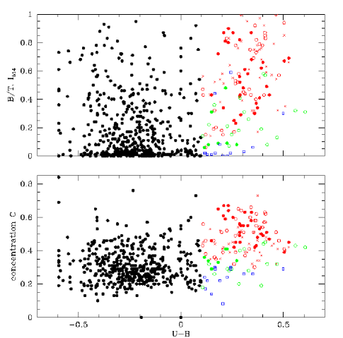
Figure 13.— Bulge/total ratio and concentration parameter $C$ measured in the $I_{814}$ images versus restframe $U-B$ color. Both quantitative morphology parameters confirm the visual assessment that red galaxies tend to be bulge-dominated with high central concentrations, while blue galaxies are more disky with lower concentrations. Red galaxies are coded for morphological type as in Figure 10: red = spheroidals; green = disks; blue = DIFRGs. Within the red population, morphological type is further correlated with concentration: low concentration and low B/T galaxies are disks or diffuse DIFRGs; high B/T galaxies are SRGs.

It is clear that color and concentration are correlated: galaxies form two distinct groups in both quantities, showing that color bimodality also mirrors quantitative structure. Blue galaxies have low concentrations and are largely clustered around pure exponential disks, with a tail to more concentrated galaxies. Red galaxies have high concentrations, and show a range in $B/T$ above $\sim 0.2$. Even in the red galaxies, few objects are found with a pure bulge or pure $r^{1/4}$ profile. This correlates with the findings of Im et al.  (2001), using GSS galaxies down to $I=22$, that morphologically normal pure E’s and E/S0’s actually exhibit a wide range in $B/T$. The threshold in that paper was set at $B/T>0.4$, which recovers most E and E/S0 galaxies based on the data here. Our results also agree with Bell et al.  (2003b), who used the Sersic $n$ index to measure the concentration of distant GEMS galaxies, obtaining the same conclusions as from visual classifications.

For red galaxies, our morphological typing is confirmed by quantitative structural measurements. Sb and edge-on disks (green points) have lower concentrations on average than spheroidal types (red points). DIFRGs (blue points) have yet lower concentration; in fact the DIFRGs are clearly unusual, since they violate the relation between concentration and color seen from blue galaxies through transition objects to red SRGs. We also examined the relation of red/blue color and morphological type to asymmetry index, but found no clear correlation (see also Wu 1999; Wu, Faber & Lauer 2003).

The color-concentration relationship for distant galaxies in Figure 13 is very similar to that found for galaxies at low redshift. As an indicator of concentration, Blanton et al.  (2003) used a single-component Sersic fit to the photometric profiles of SDSS galaxies (Sersic $n=1$ for exponential profiles and 4 for de Vaucouleurs profiles). Blue SDSS galaxies are strongly clustered around $n=1$, while red galaxies are more concentrated and range from $n=2.5$ to 4. Bell et al.  (2003b) studied SDSS galaxies using the inverse Petrosian ratio $C_{r}$, defined as $r(90)/r(50)$, and found similar results. From both near and distant studies, then, it appears that high central concentration is a prerequisite for residency on the red sequence, at least for galaxies that are red because of old stellar populations rather than dust.

Figure 13 shows that a highly concentrated light component is also present in some blue galaxies. For fitting purposes, that component is called a “photo-bulge” in the terminology of Simard et al. (2002), but it is not necessarily a true bulge in the sense of an old, red spheroidal stellar population. Koo et al.  (2004) have examined GSS galaxies individually to identify morphologically normal bulges. Almost without exception, true bulges are found to be red compared to the surrounding galaxy, while genuine blue bulges are rare. Im et al. (2001) found that blue centers live in galaxies with higher asymmetry, and that these blue-centered galaxies have small masses and central bursts of star formation. We discuss the colors of “bulges” in blue galaxies further in Section 5.7.

5.6. Color and surface brightness

A stellar population fades significantly as it reddens with age. B03 showed that because the most luminous red galaxies are brighter than the blue galaxies, the red galaxy population found in their survey cannot be produced by fading of the observed blue galaxies. Our color-magnitude distribution is similar and supports this result, as does the color-stellar mass distribution of Figure 11. Given the difference in structure between red and blue galaxies, it is also useful to look at the relation between color and surface brightness.

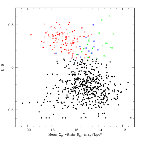
Figure 14.— Mean surface brightness vs. total $U-B$ color. $\Sigma_{B}$ is the mean B surface brightness within $R_{hl}$ in magnitudes per kpc². Points are coded for morphological type as in Figure 10. Surface brightness is strongly correlated with red galaxy morphological type: spheroidals (red) have highest $\Sigma_{B}$, DIFRGs (blue) are lower, and edge-on disks (green) are lower still.

We define a measure of mean surface brightness within the half-light radius $R_{hl}$ in kpc, $\Sigma_{B}=M_{B}+2.5~{}{\rm log}~{}2+2.5~{}{\rm log}~{}\pi R_{hl}^{2}$, which is applicable to all galaxies independent of bulge/disk ratio. Figure 14 shows the relation between galaxy color and surface brightness. Red and blue galaxies have rather different distributions in surface brightness, and in the red galaxies, surface brightness is strongly correlated with morphological class.

Among the blue galaxies, there is a tail of high surface brightness objects with mean $\Sigma_{B}<-17$. These tend to be small, compact galaxies, similar to those described by Phillips et al.  (1997). Aside from these compact galaxies, red spheroidal galaxies have a typical mean surface brightness that is higher than blue galaxies by $\sim 1.5$ magnitudes. This division is similar to the correlation between color and concentration and is clearly associated. When converted to mass surface density, the difference is even higher.

Within the red population, spheroidal red galaxies (red points) have much higher surface brightness on average than disky galaxies (green points) and diffuse red galaxies (blue points), by $\sim 2$ magnitudes. The division in surface brightness is quite striking – of course, surface brightness was one criterion used in the morphological classification – and suggests that surface brightness might be useful as a proxy for morphological type among red galaxies. The edge-on disks are quite low in surface brightness and this is probably a major reason that they are more difficult to find at higher redshifts, since surface brightness selection can have a strong effect on redshift distribution of a sample (Simard et al. 1999).

The surface brightness division is further proof that the observed blue galaxies cannot redden and fade into the observed red galaxies. The predecessors of high surface brightness red galaxies would have to be large objects with much higher SB than nearly all blue objects that we see.

5.7. Color-magnitude diagrams of bulges versus disks

The photometric decompositions by Simard et al.  (2002) make it possible to plot color-magnitude diagrams for bulges and disks separately. These are shown in Figure 15, where points are color-coded by the integrated color of the whole galaxy. For many objects with low $B/T$, the bulge color is not well measured, and these are shown as small points.

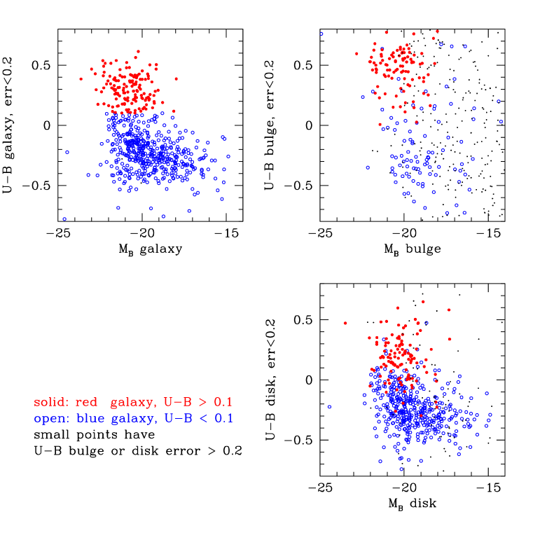
Figure 15.— Color-magnitude diagrams separately for bulges, disks, and total galaxies. Points are coded by integrated total galaxy color: red galaxies are red filled circles, blue galaxies are blue open circles. Red and blue galaxies behave oppositely in this figure. Red-population galaxies show an internal color gradient in the sense that bulges are redder than disks (i.e., the inner parts are redder than the outer parts), consistent with the run of color in local early-type galaxies. Blue galaxies show less change between disk and bulge, but, when bulges are well measured, they appear to be systematically bluer than surrounding disks. This is consistent with the conclusion that the “bulges” in blue galaxies are in fact central star-forming regions.

For galaxies with reliable bulge/disk decompositions, there is a distinct difference in behavior between red and blue galaxies. Red galaxies have luminous red bulges, with mean bulge color $U-B=0.5$, significantly redder than the mean total color of 0.35, and much redder than the mean disk color of 0.20. These are bulges in the traditional sense: spheroids with old stellar populations. Disk components bluer than the bulges imply a radial color gradient in the sense that the outer parts are bluer, in agreement with local early-type galaxies. The physical origin of these color gradients could be that the outer parts are younger, more metal-poor, or both.

The behavior of blue galaxies is opposite. Most of the “bulges” in these systems are quite blue, with mean color $U-B=-0.3$, which corresponds to vigorous star formation. Furthermore, Figure 15 shows that blue central components are systematically bluer than their outer disks. Both facts support the notion that blue galaxies with blue “bulges” are actually hosting central regions that are actively forming young stars. For example, the distant compact narrow emission-line galaxies of Guzman et al.  (1998) tend to have a high bulge fraction, but colors and $M/L$ indicating a central starburst.

A final fact, noted by Koo et al.  (2004) and visible in Figure 15, is that even the brightest blue “bulges” are actually about 1 magnitude dimmer than red bulges. Since a stellar population both fades and reddens as it ages, these blue centers cannot be the progenitors of the observed red $r^{1/4}$ bulges; they are too faint. If after fading, the blue center will deviate from local relations for luminous early-type bulges, then it cannot be a proto-luminous bulge, though it could perhaps produce a fainter or exponential bulge as found in nearby late type galaxies. Because we do not find any sufficiently bright concentrated blue sources, and few of intermediate color, we conclude that either the observed red bulges formed well before $z=1$ (see also Abraham et al.  1999), or that massive bulge formation involves growth of mass by mergers after $z=1$, or that massive bulge formation below $z=1$ is happening in sites of highly obscured star formation. These conclusions for red bulges parallel the conclusions on the formation of entire gaalxies in the red population reached by B03.

5.8. Line emission versus type and color

Most evidence up to this point indicates that, to first order, the distant red and blue populations are composed of galaxies that broadly resemble their low-$z$ counterparts. We might therefore also expect to find a strong trend between restframe color and star-formation rate, as seen in local galaxies. This is confirmed in Figure 16, which shows the log restframe equivalent width (EW) of each galaxy’s strongest emission line plotted against galaxy color. The strongest line is usually H$\alpha$ 6563 at very low $z$, [O iii] 5007 at $z\sim 0.5$, and [O ii] 3727 at $z>0.6$. Strength has been defined here as highest intensity in DN units, not in EW, although the two are closely related. The median error in restframe EW is 6.2 Å, and the median error on log EW is 0.08 dex.

Figure 16 shows the expected decline in EW at redder color for the sample as a whole, and an approximately linear relation between log EW and color, with substantial scatter. We can further ask if there is any trend between EW and morphology for the red galaxies. In Table 4 we show the median EW by morphological type for galaxies with well measured EWs.

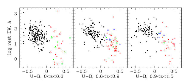
Figure 16.— Log equivalent width in Å of the strongest observed emission line versus $U-B$ restframe color, in three redshift bins. EW is strongly related to color for blue galaxies, perhaps less so for red. Red galaxies are coded for morphological type as in Figure 10: red = spheroidals; green = disks; blue = DIFRGs. Diffuse red galaxies (blue points) have generally higher emission than spheroidal red galaxies, suggesting that DIFRGs are dust-reddened rather than old.

Table 4Median emission EW for galaxies by morphological class

Type	Number	median	median
		$z$	EW, Å
SRGs (E/S0/Sa/small)	100	0.809	6.6
SRGs, $z>0.7$	59	0.878	7.5
Sb/edge-on	21	0.604	11.8
DIFRGs	13	0.814	31.3
Blue, $U-B<0.1$	411	0.632	45.1

Because the diffuse red galaxies are found only at $z>0.64$, we also tabulate the EW for spheroidal red galaxies with $z>0.7$ to make a fairer comparison. At $z>0.7$, the strongest-line EWs all refer to [O II] 3727. The median EW of diffuse red galaxies is four times higher than that of spheroidal red galaxies, confirming the impression seen in Figure 16. The DIFRGs are bluer than the SRGs, so can be expected to have higher emission given the color-EW relation, but Figure 16 suggests that the DIFRGs also lie at higher EW than the mean relation. The median EW of DIFRGs is high enough to indicate reasonably active star formation. We conclude that DIFRGs are not dominated by old stellar populations, and are reddened mainly by dust. However, since they do not have the characteristic appearance of the edge-on disks, they are a distinct, new class.

5.9. Scatter in color on the red sequence

We have seen that the red population contains a fair range of morphologies. Most objects are morphologically similar to nearby early types from E to Sa, but dust-reddened, irregular, and interacting objects can also fall on the red side of the color bimodality. This range of morphology could produce scatter in other properties, such as color. Red-sequence cluster galaxies generally fall on a tight color-magnitude relation (CMR), both locally (Bower et al.  1992) and at high redshift (van Dokkum et al.  2000). It is clear from Figure 10 that our sample of red field galaxies does not obey a perfectly narrow color-magnitude relation, nor does it have an obvious slope. However, measuring the slope and scatter are not easy because the distribution of galaxies about the red sequence is asymmetric. On the blue side of the peak, the distribution of points blends into the red wing of blue galaxies, and the presence of these objects will increase the apparent scatter of the red sequence per se unless these objects are allowed for or the sample is truncated.

B03 dealt with this by assuming a fixed CMR slope, truncating the sample to $U-V_{AB}>1.0$, and calculating a robust biweight estimator (Beers et al.  1990) of the evolving CMR zeropoint and the scatter on the red sequence. They found a Gaussian scatter on the red sequence of 0.15 mag in $U-V$ rest, or 0.09 mag transformed to $U-B$ rest, which they attributed largely to photometric redshift error. If the CMR zeropoint evolution were not subtracted, the scatter would increase only marginally to $\sim 0.10$ mag in $U-B$. We carried out a similar calculation by truncating our sample to $U-B>0.1$, the trough of the color distribution, and computing the biweight scatter. We find a scatter of 0.116 mag. This number changes only slightly to 0.112 mag when we exclude the $z<0.4$ objects with poorer K-correction, and does not change if we subtract a CMR slope in $U-B$ of 0.04 (van Dokkum et al. 2000). The scatter in $U-B$ for only spheroidal morphological types is nearly as large, 0.108 mag, and is reduced only to 0.100 mag when $z<0.4$ objects are excluded; subtracting a CMR slope again does not change the scatter.

Our CMR scatter is therefore comparable to that of B03. While our K-corrections are less accurate since we have fewer filters, we eliminate the errors due to scatter in photometric redshifts. The derived scatter is large compared to the known sources of error, which were enumerated in Section 4. Median errors of measurement in $V-I$ are only 0.055 mag, which converts to 0.03-0.04 mag in $U-B$ for a typical galaxy in the range $z=0.4$-1.0. Correcting the raw scatter of 0.112 mag for this observational error yields a net true scatter of 0.105 mag.

The other potential source of error is the K-correction in converting apparent $V-I$ to restframe $U-B$. The errors inherent in K-correction are small in the redshift interval $z=0.4$-1.0 because $U$ and $B$ transform almost directly into $V$ and $I$ at $z=0.8$. We have checked this by identifying groups of red galaxies within individual redshift peaks. Within a peak, comparing the behavior of the apparent color-magnitude relation in $V-I$ vs. $I$ to the C-M relation in $U-B$ vs. $B$ separates the scatter in the measured apparent colors from the scatter introduced by the K-correction procedure.

This test shows that our scatter in the red sequence colors has two causes. In the redshift peaks at $z=0.56$, 0.65, 0.81, 0.91, and 0.99 the apparent $V-I$ colors have a scatter of $\sim 0.1-0.2$ mag. The scatter in $V-I$ increases with redshift, in part due to the changing transformation of rest to apparent colors; at $z\sim 0.9$, the slope of $U-B/V-I$ is 0.6. Here the K-correction procedure works well, and the scatter in $U-B$ is clearly due to input scatter in $V-I$. In the redshift peak around $z=0.28$, the red galaxies form a tighter relation in $V-I$ vs. $I$, but the K-correction at this low redshift causes $U-B$ to be a stronger function of $V-I$ with slope 1.0, amplifying photometric errors and the scatter in $U-B$. The upshot is that, beyond $z=0.4$, the scatter is real and reflects real scatter in input $V-I$.

The salient conclusion is that the scatter in the color of galaxies in the red population, 0.10 mag in $U-B$ in the range $z=0.4$-1.0, is intrinsic and not due to observational error. Our scatter of 0.10 mag is close to the 0.09 ($U-B$) mag found by B03 based on their extensive 17-filter ground-based photometry. While the scatter in the CMR of both local and high-$z$ cluster galaxies is small, $\sim 0.03$-0.04 mag when converted to $U-B$ (Bower, Lucey, & Ellis 1992; van Dokkum et al.  2000), the scatter in a local sample of field E/S0 galaxies is larger, $\sim 0.06$ mag (Schweizer & Seitzer 1992). The local scatter is increased further, to 0.10 mag, by including all Hubble types and not correcting for internal extinction, as shown using RC3 galaxies below in Section 6. Notably, the scatter of DEEP1 red galaxy $U-B$ color is significantly larger than the scatter in DEEP1 red bulge color of only $\sim 0.03$ mag (Koo et al.  2004). We conclude that the red-sequence scatter we and B03 find is comparable and reflects real scatter in red field galaxy colors, both nearby and at high redshift.

6. Comparison to local data

We conclude this discussion of distant galaxies by comparing to the color-magnitude diagram of local galaxies as represented in the RC3. Figure 17 plots the CM diagram of galaxies in the RC3 (de Vaucouleurs et al.  1991) with integrated $U-B$ measurements, Galactic extinction $A_{B}<0.3$, and apparent magnitude $B_{T}^{0}<13.5$, to which the RC3 is reasonably complete. Absolute magnitudes are computed from $B_{T}$ and radial velocity in the CMB frame. Galaxies with $v_{CMB}<0$ are excluded. We plot total magnitude $M_{B}$ and color $(U-B)_{T}$, after correcting for Galactic extinction but not for internal extinction, in order to be comparable to the distant galaxy sample.

Use of the RC3 data as a local sample has two advantages. First, if we have correctly reproduced the $UB$ system for distant galaxies, no further color or aperture corrections are needed, as the RC3 galaxies are on that system. Second, most RC3 galaxies have Hubble types, which allows us to characterize the morphologies of local red-sequence galaxies in the same terms that we have set up for distant red galaxies in Section 5.4.

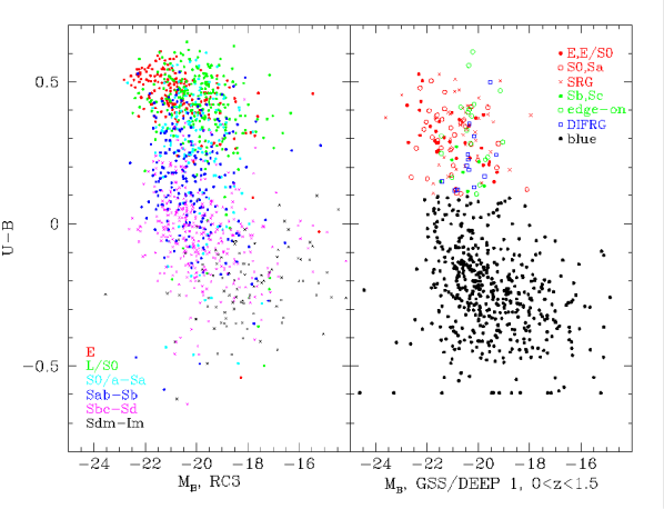
Figure 17.— Color-luminosity diagram for RC3 galaxies compared to DEEP1/GSS galaxies. Panel (a): RC3 galaxies with $U-B$ values, integrated $B$ magnitudes, redshifts, and $B_{T}^{0}<13.5$. Color codes for RC3 morphological T-type: red = E; green = L; cyan = S0/a and Sa; blue = Sab-Sb; magenta = Sbc-Sd; black = Sdm-Im. The local red seqence shows the well known slope versus magnitude. It is dominated by Hubble types E-Sa, similar to the distant red population. (b) The CM diagram for DEEP1/GSS galaxies to the same scale. Red galaxies are coded by morphological type as in Figure 10.

Figures 9 and 17(a) demonstrate the same sort of color bimodality identified in local SDSS galaxies (e.g., Strateva et al.  2001, Hogg et al.  2003, Kauffmann et al.  2003). The red population peaks around $U-B=0.45$ and shows the well known early-type color-magnitude relation. The red peak is clearly divided from the blue galaxies, which peak separately around $U-B=-0.05$. No comparable color-magnitude relation is visible for red galaxies in our DEEP1/GSS data, but B03 show one clearly out to $z\sim 1$ (with local slope). Our sample may be too small to show a relation given the large scatter.

The right-hand side of Figure 17 compares the CM diagram of GSS galaxies to the same scale. Plotting them side-by-side highlights the color evolution that has occurred in galaxies since $z\sim 0.7$, which is also shown in Figure 9. The peak of the red population has shifted redward with time by about 0.11 mag in $U-B$, the valley has moved by the same amount, and the blue peak has shifted by about 0.24 mag. Selection effects cause faint galaxies to be missing from both distant and local samples, although the effects act in the same direction in both samples. Comparing the distribution of points and the color histograms of Figure 9 suggests that the RC3 sample of blue galaxies is more heavily weighted toward brighter (thus redder) galaxies than the DEEP sample, which exaggerates the evolution. The color evolution of blue galaxies can be measured more reliably with better local samples, and with larger distant samples which measure evolution internal to the samples, from COMBO-17 and from DEEP2 (Willmer et al.  2004, in preparation).

Our color evolution of 0.11 mag in $U-B$ for the red population, from its median redshift of 0.8 to now, can be compared to the color evolution of red sequence galaxies measured by B03. Their Figure 2 shows an evolution from $z=0.8$ to 0.25 of 0.26 mag in $U-V$, and extrapolates to 0.35 mag to $z=0$, corresponding to 0.16 and 0.22 mag in $U-B$ respectively. Both numbers are larger than what we find. However, Figure 2 of B03 also shows that their red galaxies at $z=0.3$ are already redder than the colors of local galaxies from SDSS. In contrast, the color evolution from the COMBO-17 red galaxies at $z=0.8$ to SDSS galaxies at $z=0.05$ is only 0.15 mag in $U-V$ directly, or 0.1 mag converted to $U-B$, which agrees with our result. B03 noted that aperture effects may have caused their low-redshift galaxy colors to be too red, which could explain the difference. The color evolution that we find is consistent with the small color evolution found by Gebhardt et al.  (2003) and by Koo et al.  (2004), and is only half that predicted by passive evolution models with $z_{form}\sim 3$. The amount of color evolution in red galaxies is critical in determining their stellar population histories and the amount of mass buildup on the red sequence. These questions will be addressed with larger samples and better restframe colors in future DEEP2 papers.

Figure 17(a) shows Hubble types for RC3 galaxies. The RC3 red sequence is composed mainly of E and S0 galaxies, while Sa galaxies are centered on the valley between the peaks. The local population redder than the valley minimum therefore contains mostly Hubble types E to S0, with a smattering of Sa’s. This resembles the makeup of the distant red population, which consists mainly (75%) of spheroid-dominated SRGs (Section 5.4, also Bell et al.  2003b).

However, roughly 25% of our distant red galaxies are not typed as SRGs. Of these, nearly all are either edge-on disks (some of which may be SRGs) or are DIFRGs. We have examined the RC3 sample to see if such objects are present on the local red sequence as well. A small contaminating population of intermediate Hubble types (Sab to Sc) is indeed found, at the few percent level, and most of these interlopers are edge-on or close to it and are likely reddened by dust. These are presumably the analogs of our distant edge-on galaxies. The number of these edge-on middle Hubble types is about the same in both the DEEP1 and RC3 samples as a fraction of the blue galaxy population.

The DIFRGs are another matter. We have seen that they tend to populate the valley between the red and blue population, the region that locally is occupied by Sa’s. However, DIFRGs structurally do not resemble Sa’s, because they completely lack a large spheroid. The most plausible local analogs to DIFRGs in structure are types Sc and later. But there are only three Sc’s on the entire RC3 subsample red sequence (out of 517 galaxies), and all three are edge on and dust-reddened. DIFRGs, we have noted, are distinct from classic edge-on disks, because they are not as flattened. The most plausible local red-sequence analog to DIFRGs is perhaps the dusty, irregular starburst galaxy M82, which has $U-B=0.28$ and whose light is not strongly concentrated in the $B$-band (although it is more concentrated in $K$ images). M82 itself is highly inclined but is likely to be reddened even if not viewed edge-on. Other than M82, there do not seem to be common local red-sequence analogs to distant DIFRGs, which is consistent with their apparent disappearance at low redshift in our sample, as noted in Section 5.4. It is possible that DIFRG analogs could exist locally at the same color as high-z DIFRGs, $U-B\sim 0.15$. In that case they would not be on the local red sequence, but would be a minority within the red edge of the blue population, which is mostly disk galaxies with bulges in the RC3 sample. Thus, both the nature of high-z DIFRGs and what they evolve into remain unclear.

The next point to examine is the color scatter of galaxies about the RC3 red sequence. Applying the same method used in Section 5.8 to reject outliers, we find that the biweight scatter about the red peak is 0.10 mag in $U-B$ for all galaxies with $U-B>0.2$, if no CM relation is subtracted, and decreases insignificantly when a CM relation of slope 0.025 is subtracted and the sample is cut by a line 0.25 mag blueward of the CM relation. To parallel the treatment of the distant samples, all Hubble types are included, and no corrections for internal reddening have been made. This RC3 scatter is essentially the same as the 0.11 mag we find for the GSS galaxies (with no CM relation subtracted), and the 0.09 mag found by B03 (with an evolving CM relation subtracted). We conclude that an rms scatter in $U-B$ of $\sim 0.10$ mag typifies field red-sequence galaxies at all redshifts below $z\sim 1$. This is significantly larger than the scatter of 0.03-0.04 found for red, early-type cluster galaxies, both near and far (e.g., Bower et al.  1992; van Dokkum et al.  2000).

Finally, the reader may have noticed that the number of red galaxies relative to blue galaxies is only about half as large in the GSS CM diagram as that in the RC3. One factor that discriminates against distant red galaxies is the R-band selection limit, shown in Figure 10, which preferentially selects against red galaxies at high redshift. On the other hand, a real increase in the number of red galaxies with time would be consistent with the increase in total red stellar mass reported by B03 below $z=1$. This topic is discussed further in Willmer et al.  (2004, in preparation), where we derive luminosity functions from DEEP samples.

7. Conclusions

The DEEP1 survey of the Groth Strip provides redshifts and spectra for over 600 galaxies out to $z\sim 1$, with HST/WFPC2 imaging in two filters; the median redshift is $z=0.65$. Large scale structure walls are visible in the space distribution to $z\sim 1$.

The DEEP1 galaxy sample shows a bimodality in the color-magnitude diagram similar to that found locally in the SDSS (Blanton et al.  2003; Kauffmann et al.  2003) and to $z\sim 1$ in COMBO-17 (B03). The brightest red galaxies are somewhat more luminous than the brightest blue galaxies, so that the observed blue galaxies cannot fade to produce the brightest red galaxies, as discussed by B03. This difference between the most luminous red and blue galaxies is even stronger in terms of stellar mass, as shown in Figure 11. The processes of star formation, quenching, and mass assembly in red galaxies will be studied at greater length in future surveys, including DEEP2 measurements of the luminosity function (Willmer et al.  2004, in preparation).

The present sample does not permit a measurement of the red galaxy color-magnitude relation slope, but we can measure the scatter in color of distant red field galaxies. We find a scatter of 0.11 mag in restframe $U-B$, even if only spheroidal types are included. This scatter is comparable to that found in COMBO-17 (B03), and in a sample of red galaxies selected from the RC3, but larger than found in local or high-redshift early-type cluster galaxies (Bower et al.  1992; van Dokkum et al.  2000).

DEEP1 galaxies have structural measurements from HST imaging of the Groth Strip (Simard et al.  2002). Red galaxies are generally more centrally concentrated than blue galaxies, as found at low redshift in the SDSS (Blanton et al.  2003). The bulk of red galaxies have red stellar bulges, while blue galaxies generally have exponential profiles. Red bulges are brighter than blue starforming centers, so that the same problem of progenitors occurs for red bulges as for red galaxies in toto.

We have classified red galaxies into three main groups: spheroidal red galaxies (SRGs), edge-on disks, and diffuse red galaxies (DIFRGs). These classifications correlate well with objective measures of central concentration. The SRGs include objects which resemble local spheroid-dominated galaxies of type E, S0 and Sa; these are presumably red due to old, metal-rich stellar populations. The edge-on disks are presumably reddened by dust.

The DIFRGs are the most puzzling category: these do not have a strong central concentration, are not edge-on, and resemble local diffuse galaxies such as Magellanic irregulars, but of course are both more luminous and redder. They are not obviously interacting or merging. Our measurements of line emission from the DIFRGs indicate that they are star-forming and likely reddened by dust rather than old stellar populations. Based on an examination of red galaxies in a local sample drawn from the RC3, there is no common type of local red galaxy with morphology similar to the DIFRGs; M82 may be the best analog. The GEMS survey of red galaxy morphologies at $0.65<z<0.75$ did not note DIFRGs as a class (Bell et al.  2003b), but this may be influenced by the relatively low redshift range studied. The DIFRGs in the DEEP1 sample are all at $z>0.65$, above the median redshift of our survey, suggesting that DIFRGs are more common at high redshift. Studies of extremely red objects (EROs) in the GOODS-S field indeed find fewer spheroidals and a larger fraction of irregular and “other” types at $z>1.5$ (Moustakas et al.  2004). If in fact DIFRGs are similar to dusty EROs, they provide an opportunity to study the ERO phenomenon at lower redshifts, where nebular features are accessible to optical spectroscopy.

This paper has focused mainly on the properties of distant red-population galaxies. Principal unanswered questions concerning them are the color evolution of red galaxies, the manner in which galaxies evolve onto the red sequence, how their numbers and total stellar mass change with time, and the nature of diffuse red galaxies and their descendants. Though blue galaxies are not highlighted here, the evolution in their properties may be even greater than that of red galaxies, given their color evolution. A worthy project for the future will be correlating the color evolution of blue galaxies with other properties such as mass, star formation rate, and structure, and studying the entire suite of properties as a function of location in the color-magnitude diagram.

References

- (1)
- (2)
- (3) Abazajian, K., et al. 2003, AJ, 126, 2081
- (4)
- (5) Abraham, R.G., et al. 2004, AJ, 127, 2455
- (6)
- (7) Abraham, R.G., Ellis, R.S., Fabian, A.C., Tanvir, N.R., & Glazebrook, K. 1999, MNRAS, 303, 641
- (8)
- (9) Abraham, R.G., Valdes, F., Yee, H.K.C., & van den Bergh, S. 1994, ApJ, 432, 75
- (10)
- (11) Beers, T.C., Flynn, K., & Gebhardt, K. 1990, AJ, 100, 32
- (12)
- (13) Abraham, R.G., & van den Bergh, S. 2001, Science, 293, 1273
- (14)
- (15) Bell, E.F., Wolf, C., Meisenheimer, K., Rix, H.-W., Borch, A., Dye, S., Kleinheinrich, M., & McIntosh, D.H. 2003a, astro-ph/0303394, ApJ, in press (B03)
- (16)
- (17) Bell, E.F., et al. 2003b, ApJ, 600, L11
- (18)
- (19) Bell, E.F., McIntosh, D.H., Katz, N., & Weinberg, M.D. 2003c, ApJS, 149, 289
- (20)
- (21) Benson, A.J., Bower, R.G., Frenk, C.S., Lacey, C.G., Baugh, C.M., & Cole, S. 2003, ApJ, 599, 38
- (22)
- (23) Binney, J. 2004, MNRAS, 347, 1093
- (24)
- (25) Blanton, M.R., et al. 2001, AJ, 121, 2358
- (26)
- (27) Blanton, M.R., et al. 2003, ApJ, 592, 819
- (28)
- (29) Bower, R.G., Lucey, J.R, & Ellis, R.S. 1992, MNRAS, 254, 601
- (30)
- (31) Brinchmann, J., et al. 1998, ApJ, 499, 112
- (32)
- (33) Broadhurst, T.J., Ellis, R.S., Koo, D.C., & Szalay, A.S. 1990, Nature, 343, 726
- (34)
- (35) Calzetti, D., Kinney, A.L., & Storchi-Bergmann, T. 1994, ApJ, 429, 582
- (36)
- (37) Cimatti, A., et al. 2002, A&A, 381, L68
- (38)
- (39) Cimatti, A., et al. 2003, A&A, 412, L1
- (40)
- (41) Cohen, J.G. 2001, AJ, 121, 2895
- (42)
- (43) Cohen, J.G., Cowie, L.L., Hogg, D.W., Songaila, A., Blandford, R., Hu, E.M., & Shopbell, P. 1996, ApJ, 471, L5
- (44)
- (45) Cohen, J.G. et al. 2000, ApJ, 538, 29
- (46)
- (47) Coil, A., et al. 2004, ApJ, 609, 525
- (48)
- (49) Coleman, G.D., Wu, C.-C., & Weedman, D.W. 1980, ApJ, 43, 393
- (50)
- (51) Colless, M., et al. 2001, MNRAS, 328, 1039
- (52)
- (53) Connolly, A.J., Szalay, A.S., Koo, D., Romer, A.K., Holden, B., Nichol, R.C., & Miyaji, T. 1996, ApJ, 473, L67
- (54)
- (55) Crampton, D., Le Fèvre, O., Lilly, S.J., & Hammer, F. 1995, ApJ, 455, 96
- (56)
- (57) de Vaucouleurs, G., de Vaucouleurs, A., Corwin, H.G., Buta, R.J., Paturel, G., & Fouque, P. 1991 The Third Reference Catalog of Galaxies (RC3), New York: Springer Verlag
- (58)
- (59) Doroshkevitch, A.G., et al. 1996, MNRAS, 283, 1281
- (60)
- (61) Ellis, R.S., Colless, M., Broadhurst, T., Heyl, J., & Glazebrook, K. 1996, MNRAS, 280, 235
- (62)
- (63) Fukugita, M., Shimasaku, K., & Ichikawa, T. 1995, PASP, 107, 945
- (64)
- (65) Gebhardt, K., et al. 2003, ApJ, 597, 239
- (66)
- (67) Granato, G.L., de Zotti, G., Silva, L., Bressan, A., & Danese, L. 2004, ApJ, 600, 580
- (68)
- (69) Groth, E.J., Kristian, J.A., Lynds, R., O’Neil, E.J., Balsano, R., Rhodes, J., & WFPC-1 IDT. 1994, BAAS, 26, 1403
- (70)
- (71) Guzman, R., Jangren, A., Koo, D.C., Bershady, M.A., & Simard, L. 1998, ApJ, 495, L13
- (72)
- (73) Hogg, D.W., et al. 2003, ApJ, 585, L5
- (74)
- (75) Hopkins, A.M., Connolly, A.J., & Szalay, A.S. 2000, AJ, 120, 84
- (76)
- (77) Im, M., et al. 2002, ApJ, 571, 136
- (78)
- (79) Kauffmann, G., et al. 2003, MNRAS, 341, 54
- (80)
- (81) Kinney, A.L., Calzetti, D., Bohlin, R.C., McQuade, K., Storchi-Bergmann, T., & Schmitt, H. R. 1996, ApJ, 467, 38
- (82)
- (83) Koo, D.C., et al. 1996, ApJ, 469, 535
- (84)
- (85) Koo, D.C., et al. 2004, ApJ, submitted
- (86)
- (87) Kroupa, P., Tout, C.A., & Gilmore, G. 1993, MNRAS, 262, 545
- (88)
- (89) Le Fèvre, O., Crampton, D., Hammer, F., Lilly, S.J., & Tresse, L. 1994, ApJ, 423, L89
- (90)
- (91) Le Fèvre, O., Hudon, D., Lilly, S.J., Crampton, D., Hammer, F., & Tresse, L. 1996, ApJ, 461, 534
- (92)
- (93) Le Fèvre, O., et al. 2004, astro-ph/0402203
- (94)
- (95) Lilly, S.J., Hammer, F., Le Fèvre, O., & Crampton, D. 1995a, ApJ, 455, 75
- (96)
- (97) Lilly, S.J., Tresse, L., Hammer, F., Crampton, D., & Le Fèvre, O. 1995b, ApJ, 455, 108
- (98)
- (99) Lin, H., et al. 1999, ApJ, 518, 533
- (100)
- (101) Madgwick, D.S., et al. (2dFGRS Team) 2002, MNRAS, 333, 133
- (102)
- (103) Madgwick, D.S., et al. 2003, ApJ, 599, 997
- (104)
- (105) Moriondo, G., Cimatti, A., & Daddi, E. 2000, A&A, 364, 26
- (106)
- (107) Moustakas, L.A., et al. 2004, ApJ, 600, L131
- (108)
- (109) Oke, J.B., et al. 1995, PASP, 107, 375
- (110)
- (111) Phillips, A.C., et al. 1997, ApJ, 489, 543
- (112)
- (113) Phillipps, S., Drinkwater, M.J., Gregg, M.D., & Jones, J.B. 2001, ApJ, 560, 201
- (114)
- (115) Rhodes, J., Refregier, A., & Groth, E.J. 2000, ApJ, 536, 79
- (116)
- (117) Rix, H.-W., et al. 2004, astro-ph/0401427
- (118)
- (119) Schlegel, D.J., Finkbeiner, D.P., & Davis, M. 1998, ApJ, 500, 525
- (120)
- (121) Shepherd, C.W., et al. 2001, ApJ, 560, 72
- (122)
- (123) Simard, L., et al. 1999, ApJ, 519, 563
- (124)
- (125) Simard, L., et al. 2002, ApJS, 142, 1, (Paper II)
- (126)
- (127) Steidel, C.C., Shapley, A.E., Pettini, M., Adelberger, K.L., Erb, D.K., Reddy, N.A., & Hunt, M.P. 2004, ApJ, in press
- (128)
- (129) Strateva, I., et al. 2001, AJ, 122, 1861
- (130)
- (131) Takamiya, M., Kron, R.G., & Kron, G.E. 1995, AJ, 110, 1083
- (132)
- (133) van den Bergh, S., Cohen, J.G., Hogg, D.W, & Blandford, R. 2000, AJ, 120, 2190
- (134)
- (135) van Dokkum, P.G., Franx, M., Fabricant, D., Illingworth, G.D., & Kelson, D.D. 2000, ApJ, 541, 95
- (136)
- (137) van Dokkum, P.G., et al. 2004, ApJ, 611, 703
- (138)
- (139) Vogt, N.P., et al. 2004, in preparation, (Paper I)
- (140)
- (141) Vogt, N.P., et al. 1996, ApJ, 465, 15
- (142)
- (143) Vogt, N.P., et al. 1997, ApJ, 479, L121
- (144)
- (145) Willmer, C.N.A., Koo, D.C., Szalay, A.S., & Kurtz, M.J. 1994, ApJ, 437, 560
- (146)
- (147) Willmer, C.N.A., et al. 2004, in preparation
- (148)
- (149) Wolf, C., Meisenheimer, K., Rix, H.-W., Borch, A., Dye, S., & Kleinheinrich, M. 2003, A&A, 401, 73
- (150)
- (151) Wu, K.L. 1999, PhD thesis, University of California, Santa Cruz
- (152)
- (153) Wu, K.L., Faber, S.M., & Lauer, T.R. 2003, Rev Mex A&A, 17, 241
- (154)
- (155) Yan, L., & Thompson, D. 2003, ApJ, 586, 765
- (156)
- (157) Zehavi, I., et al. 2002, ApJ, 571, 172
- (158)