Modeling the evolution of infrared luminous galaxies: the influence of the Luminosity-Temperature distribution.

Abstract

The evolution of the luminous infrared galaxy population is explored using a pure luminosity evolution model which incorporates the locally observed luminosity-temperature distribution for IRAS galaxies. Pure luminosity evolution models in a fixed $\Lambda$CDM cosmology are fitted to submillimeter (submm) and infrared counts, and backgrounds. It is found that the differences between the locally determined bivariate model and the single variable luminosity function (LF) do not manifest themselves in the observed counts, but rather are primarily apparent in the dust temperatures of sources in flux limited surveys. Statistically significant differences in the redshift distributions are also observed. The bivariate model is used to predict the counts, redshifts and temperature distributions of galaxies detectable by Spitzer. The best fitting model is compared to the high-redshift submm galaxy population, revealing a median redshift for the total submm population of $z=1.8^{+0.9}_{-0.4}$, in good agreement with recent spectroscopic studies of submillimeter galaxies. The temperature distribution for the submm galaxies is modeled to predict the radio/submm indices of the submm galaxies, revealing that submm galaxies exhibit a broader spread in spectral energy distributions than seen in the local IRAS galaxies.

1. Introduction

With an energy comparable to the optical/UV background, measurements of the far infrared background reveal it to peak at around 200$\mu m$ (Puget et al.  1996; Fixsen et al.  1998), arising from dust-reprocessing of high energy radiation and star formation and AGN activity in $z>0$ galaxies. Such obscuration could be hiding approximately half of the massive star formation activity over the history of the Universe (e.g. Blain et al.  1999a). Clearly, to unravel the cosmic history of star formation the evolution of the infrared galaxy population needs to understood.

Studies of the evolving infrared galaxy populations have typically assumed a small range of template galaxy spectral energy distributions (SEDs), or even a single SED. However, infrared galaxies span a large range in properties, with 60$\,\mu$m/100$\,\mu$m  colors spanning $\sim 0.4$ dex for a given luminosity (Soifer & Neugebauer 1991, Chapman et al.  2003a). This distribution in dust SEDs implies that substantial numbers of both extremely luminous, yet cold galaxies, as well as low luminosity, hot galaxies are found.

In a previous paper (Chapman et al.  2003a – hereafter C03) an evolving distribution bivariate in luminosity and color, $\Phi$(${\cal L}$, ${\cal C}$), was presented, providing consistency with the broad distribution of submm galaxies observed locally. This earlier paper demonstrated that flux-limited surveys in various infrared and submillimeter (submm) bands would subsume a non-negligible fraction of both cold, luminous galaxies and hot, faint galaxies, the predictions borne out in observations of low and moderate redshift IRAS galaxies, as well as microJansky radio sources. The overall conclusion of this study was that surveys which select objects at either the cold Raleigh-Jeans tail of the dust SED, or the hot Wien tail, will preferentially detect appropriately cold or hot objects for a given luminosity class, in much larger numbers than expected if the temperature distributions were not taken into account.

Figure 1.— The upper panel presents the bivariate model count from our best fit simulation at 850$\,\mu$m  (red), 170$\,\mu$m  (purple), 160$\,\mu$m (green), 70$\,\mu$m (cyan), 24$\,\mu$m (blue), and 15$\,\mu$m(yellow), compared to SCUBA and ISO counts from the literature (points). For comparison, we overlay the model counts of Lagache, Dole & Puget  (2003) as dashed lines. In the lower panel, the integrated bivariate model is compared to the Cosmic Infrared-Background of Fixen et al. (1998). The upper-limits at 12$\mu m$ and 24$\mu m$ are drawn from Scott et al. (2001).

Submm-luminous, extragalactic sources (Smail, Ivison, Blain 1997) currently provide our only means of studying the high redshift infrared galaxy population (Chapman et al. 2003b). These galaxies are now routinely detected with the SCUBA/JCMT and MAMBO/IRAM instruments, and over 200 blank field sources are now cataloged from cluster lensed surveys (see Blain et al. 2002 for a summary). The tight correlation observed locally between thermal FIR emission and synchrotron radio emission (Helou et al. 1985, Condon 1992) allows the identification of submm sources, recovering $\sim$65% of the blank field counts (Ivison et al.  2002; Chapman et al. 2003a). With spectroscopic redshifts for the submm galaxies (SMGs), the possibility exists to assess more subtle effects in our model, and to understand whether our model can explain the range in properties subsumed by the SMGs, as well as explore the implication of various selection approaches employed in submm surveys.

In this paper, the bivariate model is examined in light of the multi-wavelength counts and backgrounds, using a parameterization of pure luminosity evolution. The model is first used to explore predictions for the Spitzer Space Telescope galaxy populations in terms of their redshift, color, and temperature distributions. The model is then employed to better understand the range in properties and redshift distributions sampled by the radio-identified submm galaxy population, and the importance of the luminosity–dust temperature distribution, ${\cal L-T}$, and by extrapolation the properties of the entire submm population. All calculations are undertaken in a $\Omega_{0}=0.3$, $\Lambda_{0}=0.7$, h=0.65 cosmology.

Figure 2.— Redshift distributions at 24$\,\mu$m, 70$\,\mu$m, 160$\,\mu$m, and 850$\,\mu$m. The distributions are shown for both a deep (left) and a shallow (right) survey, in the bivariate (solid line) and single variable (dashed line) models. The effect of the bivariate distribution is to increase the numbers of both high and low-redshift sources relative to the single variable model, due to the temperature spread. The shallow survey is comparable to the expected FLS survey, with the 850$\,\mu$m survey being typical of current wide-field SCUBA surveys. The deep survey is scaled at all wavelengths by a factor of 5.

2. Evolution of the bivariate LF

The evolutionary model is anchored to the local FIR luminosity function (LF), constructed from the 1.2 Jy sample of IRAS galaxies (Fisher et al. 1995, C03). Recent work has emphasized the variation in dust temperature found in ULIRGs with T_d as low as 25 K (Chapman et al. 2002c). The adopted form of the LF represents the distribution in dust temperatures found in the 1.2 Jy sample, parametrized by the 60$\,\mu$m/100$\,\mu$m  color (a full characterization of this LF can be found in C03).

The local bivariate LF is then evolved using pure luminosity evolution with redshift. While a range of functional forms have been employed in the literature in the study of the various IR, submm and radio populations, Blain et al. (1999a,b) have demonstrated that models which are not strongly peaked, in particular those which flatten beyond a certain redshift, have problems over-predicting the submm background. While it is clear that it will not be possible to distinguish minute details of evolutionary form, this study aims to constrain its gross properties.

Figure 3.— Color-color diagrams of galaxies in a 24$\,\mu$m  flux limited survey (S${}_{24\mu m}>0.2$ mJy). The left-hand plot presents $70\mu m/160\mu m$ versus $8\mu m/24\mu m$ for the univariate case, whereas the right-hand panel presents the same distribution for the bivariate case. Objects are color-coded by redshift: $0<z<1$ (cyan), $1<z<2$ (blue), $2<z<3$ (green), $z>3$ (red).

2.1. Fitting the multi-wavelength counts and backgrounds

Studies invoking a pure density evolution of the FIR galaxy population have been shown to grossly over predict the cosmic infrared background and are hence unphysical. Other authors have considered both density and luminosity evolution of the FIR population, successfully recovering both the number counts and backgrounds (Franceschini et al. 2001; Chary & Elbaz 2001; Xu et al. 2004). However, it has been shown that these observational properties can be explained within models adopting only luminosity evolution (Blain 1999a). Given its simplicity (with reduced parameters), we adopt a similar pure luminosity evolution to examine the cosmic history of FIR galaxies.

The evolution is modeled in a simple form; $\Phi(L,{\cal C})=\Phi_{0}(L/g(z),{\cal C^{\prime}})$. The color term of our LF (${\cal C^{\prime}}$ rest frame 60$\,\mu$m/100$\,\mu$m  flux ratio) does not evolve, but rather continues to scale with FIR luminosity as found locally. C03 and Blain, Barnard & Chapman (2003) have demonstrated that this lack of significant 60$\,\mu$m/100$\,\mu$m  color evolution appears to hold at least out to moderate redshifts ($0.3<z<0.9$) in a sample of IRAS detected ULIRGs of Stanford et al. (2000). As the form of the ${\cal L-T}$ distribution remains fixed for all redshifts, the only remaining parameter is $g(z)$. It should be noted that Dunne et al. (2000) suggested that the IRAS galaxy luminosity function may be incomplete, missing cold galaxies. Recently, this conclusion has been strengthened by observations by Klaas et al. (2001) and Bendo et al. (2002; 2004). Given that the current study is tied to IRAS, this effect will accentuate the features of cold galaxies presented in this paper, although the degree of IRAS underrepresentation of cold galaxies must be quantified to fully explore this.

Adopting a Monte Carlo approach, luminous infrared galaxies are drawn randomly from the evolving distribution function. A galaxy thus selected from this model Universe is then assigned a template spectral energy distribution from the catalog of Dale et al. (2001, 2002), parameterized by the 60$\,\mu$m/100$\,\mu$m  color, and normalized to the FIR luminosity. This model scenario does not incorporate the intrinsic scatter in the FIR/radio correlation (0.2 dex), as was done in Chapman et al. (2002b; hereafter C02). Rather this study concentrates on the properties of the intrinsic dust temperature distribution which locally show a larger scatter (0.3 dex) than the FIR/radio correlation, and should be expected to dominate the high redshift radio and submm properties.

C02 adopted an evolution function with a simple power law peak, $g(z)\propto(1+z)^{4}$ out to a break redshift, and dropping thereafter as $g(z)\propto(1+z)^{-4}$, with no discontinuity in the zeroth derivative. This power-law index was chosen provided reasonable descriptions of submm and radio data, allowing a fit to the sub-mm counts and background (C02). This evolution form coupled with the bivariate model provided a reasonable fit over the submm fluxes represented by our data (5$<$S_850μm$<$15 mJy). However, the model produced too many bright submm sources, with an increasing excess of $>$20 mJy sources with increasing peak redshift. This toy model cannot be considered physical, and the culprit for the excess bright sources is found to be in the peak turnover in $g(z)$ producing a spike of luminous sources at the tip of our color-magnitude diagram (CMD) coupled with the range of T_d for each luminosity. While this peak model was useful for illustrating various selection effects (as in C03), it must be replaced with a more realistic evolution form to provide a more accurate description of the submm population and, therefore, the functional form of Blain et al. (1999b) is adopted $g(z)=(1+z)^{3/2}sech^{2}[{\rm b}\ln(1+z)-{\rm c}]cosh^{2}{\rm c}$.

Figure 4.— Comparison of our Monte Carlo representation of the evolving $\Phi$(${\cal L}$, ${\cal C}$) (blue points) to an evolving univariate model LF (red points) with a one-to-one mapping of luminosity to color. Each point represents only luminosity and thus the distributions are equal in both cases. The difference between models is apparent when flux limited surveys are defined on the model points. We overlay flux limited samplings of the model points with darker symbols. In the single variable LF model, luminosities map uniquely to fluxes and lines can be drawn which reflect fixed temperatures. The upper panels are for 8$\,\mu$m and 24$\,\mu$m, while the lower panels are for 70$\,\mu$m and 160$\,\mu$m.

In constraining the form of the above evolution model, galaxy submm/radio distributions with varying values of $b$ and $c$ were constructed and compared to the differential number count models at 850$\mu$m (Barger, Cowie & Sanders 1999) and 15$\mu$m (Elbaz et al. 1999). For particular set of values of $b$ and $c$, the number counts are scaled to minimize the residuals between the Monte Carlo simulation and the modeled number counts. For the purposes of this study, it was assumed that the models possessed an uncertainty of 0.2 dex and the resulting best values of $b$ and $c$ are $2.10^{+0.50}_{-0.60}$ and $1.81^{+0.24}_{-0.46}$ respectively. The range of parameters effectively shift the $z_{\rm peak}$ of the peak evolution function such that $z_{\rm peak}=1.8^{+0.9}_{-0.4}$.

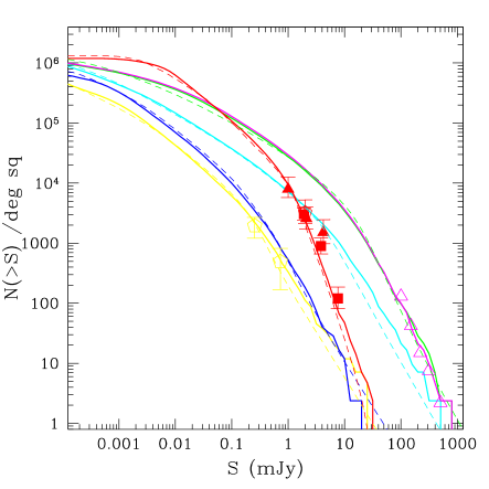
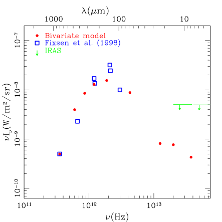
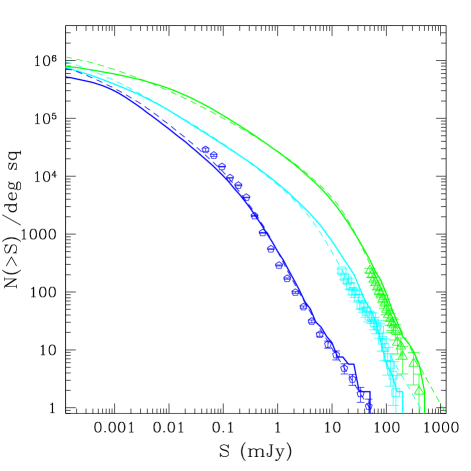
Bivariate model count from our best fit simulation at 850$\,\mu$m, 170$\,\mu$m, 160$\,\mu$m, 70$\,\mu$m, 24$\,\mu$m, and 15$\,\mu$m, are shown in the upper panel of Fig. 1. The models are overlaid on measured SCUBA (850$\,\mu$m– Blain et al. 2002) and ISO (15$\,\mu$m  – Elbaz et al. 1999; and 170$\,\mu$m– Dole et al. 2001) counts from the literature. For comparison, we overlay the model counts of Dole et al. (2003) as dashed lines, which agree remarkably well with our models. At the brightest end of the counts, our model is constrained by the length of our Monte Carlo runs, and we are dominated by small number statistics. In the lower panel of Fig. 1 presents compares the integrated flux in the bivariate model, compared to the observed Cosmic Infrared Background (CIB; Fixen et al. 1998); again, the best fit model from the counts accounts for the observed CIB distribution.

Previous modeling (C02) found a reasonable fit to the data with a peak evolution redshift of $z=3$, when all objects were assumed to have hot dust temperatures ($\sim 50$ K), similar to the local ULIRG, Arp220. The current model ties the dust temperature of a source to its luminosity as observed locally for the IRAS 1.2 Jy sample galaxies, whereby a galaxy with a FIR luminosity of 10¹² L_⊙ has T_d=35 K and dust emissivity $\beta=1.6$, as described in Dale & Helou (2002). In addition, the 60$\,\mu$m/100$\,\mu$m  color distribution observed locally is adopted in the FIR luminosity function, resulting in a tail of cold luminous galaxies which are preferentially selected with SCUBA at 850$\,\mu$m (e.g., Blain 1999b, Eales et al. 1999, Chapman et al. 2002c). As expected (see also the discussion in C02), the best-fitting peak evolution redshift must be lower if a population of luminous colder sources exists at high redshifts.

Figure 5.— Comparison of the dust temperature distributions as a function of redshift for the $\Phi$(${\cal L}$, ${\cal C}$) (solid lines) to an evolving model LF with a one-to-one mapping of luminosity to color (dashed lines). Distributions are shown for hot (red lines – T_d$>$40 K), medium (green lines – 28$<$T_d$<$33 K), and cold (blue lines – T_d$<$25 K). The panels are divided by wavelength, as indicated.

3. Predictions for spitzer and submillimeter galaxies

3.1. Redshift & color-color distributions

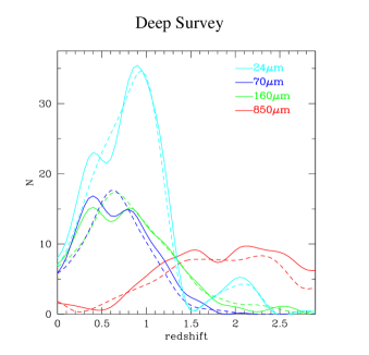
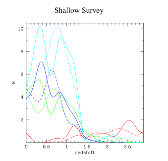
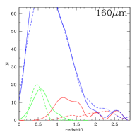
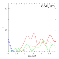
Taking our best-fit evolution functions for both the bivariate and single variable models, we predict redshift distributions for galaxy surveys at 24$\,\mu$m, 70$\,\mu$m, 160$\,\mu$m, and 850$\,\mu$m, covering an area of one square degree. We place flux density thresholds on our simulation, comparable with a shallow Spitzer observation such as the First Look Survey (http://ssc.spitzer.caltech.edu/fls). A deep survey is also analyzed, representing flux densities five times fainter in all bands (ignoring the effects of confusion in the longer wavelength beams for now). For the submm surveys, the shallow survey is set at the confusion limit of SCUBA (2 mJy). The survey reaching five times this depth will be achievable with future instruments such as ALMA.

The comparisons are shown in Fig. 2. Due to the spread in temperature at each luminosity, with increasing numbers of hot sources lying at higher redshifts and conversely colder sources at lower redshift, the effect of the bivariate distribution is to increase the numbers of both high and low-redshift sources relative to the single variable model. In considering photometric redshifts for Spitzer sources, or indeed simply trying to pre-select sub-populations of Spitzer sources with a given range in redshift or temperature properties, it is, therefore, crucial to have a calibrated estimate of the source distributions in the various color-color planes.

Figure 6.— As for the upper panel in Figure 1, but now the bivariate model is compared to the recently compiled Spitzer counts at 24$\mu m$ (blue), 70$\mu m$ (cyan) & 160$\mu m$ (green) (Dole et al. 2004; Papovich et al. 2004).

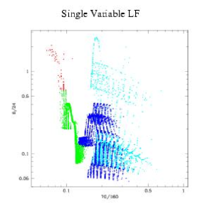
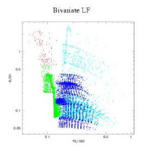
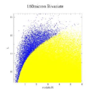
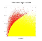
Color-color diagrams of galaxies in a 24$\,\mu$m  flux limited survey (S${}_{24\mu m}>0.2$ mJy) are shown in Fig. 3. The left-hand panel presents the distribution of galaxies assuming the univariate luminosity-temperature relation, whereas the right-hand panel presents the corresponding distribution for the bivariate case. In each panel, objects are color-coded by redshift: $0<z<1$ (cyan), $1<z<2$ (blue), $2<z<3$ (green), $z>3$ (red). It is apparent that the distribution of galaxies in the two figures is markedly different, with the introduction of a bivariate form of the luminosity function changing the relative density of galaxies in the color-color plane; this behavior is also seen in other color-color planes. Clearly, while different redshift regimes can be delineated in the color-color plane, allowing the determination of photometric redshifts for galaxies, the redistribution of galaxies in the plane due to the introduction of the bivariate distribution implies that such determinations depend on the nature of the luminosity-temperature relationship.

While our model has not yet been tuned to fit the deep, multi-wavelength Spitzer counts, it already emphasizes that the source distributions as a function of redshift and SED can vary significantly, from the bivariate case to the single temperature luminosity models. Upcoming papers will explore this issue more fully, once deep Spitzer data is available to further constrain our models.

Figure 7.— S_850μm/S_1.4GHzindices for SMGs with redshifts, compared to our model prediction, with the dashed lines corresponding to 1$\sigma$ scatter in the population of model galaxies. Note that the model includes only the range of dust temperatures observed locally in the IRAS population, whereas a variation in the radio to farIR ratio likely increases the scatter further.

In C03 we presented the baseline assumption in this model: the local S_850μm/S_1.4GHz as a function of ${\cal L}$ holds at all redshifts, simply extrapolating the local ${\cal L}-{\cal C}$ relation to the required luminosities. We have now fit this model explicitly to the pre-Spitzer submm and mid-infrared counts to constrain the evolution function, and used this tuned model to make predictions on the populations observed in the Spitzer wavelengths (8$\,\mu$m, 24$\,\mu$m, 70$\,\mu$m, and 160$\,\mu$m).

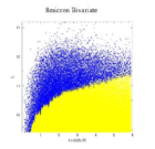
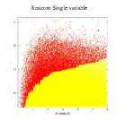
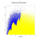
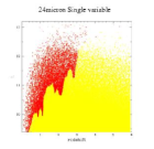
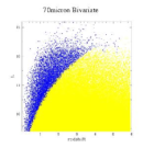
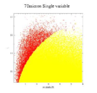
In Fig. 4, we show the L_TIR distribution as a function of redshift. Each pair of panels represents a particular waveband (8$\,\mu$m, 24$\,\mu$m, 70$\,\mu$m, and 160$\,\mu$m respectively), with the left-hand panel in a pair representing the bivariate model (blue markers) and the right-hand panel presenting the univariate case (red markers). Until we apply a flux limit to the figure (darker points), there is no difference between the visualizations since they have the same luminosity evolution formalism. Fig. 4 is our Monte Carlo representation of the evolving LF; vertical slices reveal the dual power law $\Phi$(${\cal L}$, ${\cal C}$) at each redshift.

When flux limited surveys are considered in the context of Fig. 4, differences in the two models become manifest. In the case of the single variable distribution, each L_TIR point maps uniquely to a flux for a given wavelength. However in the bivariate LF, each L_TIR point corresponds to a probability distribution of fluxes corresponding to the log-normal distribution in S_850μm/S_1.4GHz and the associated range of SED templates that can be tied to the L_TIR value. The sensitivity limits in the various bands are shown for the deepest surveys with Spitzer. The structure in the 8$\,\mu$m and 24$\,\mu$m surveys is a result of PAH bands (rest $\sim$10$\,\mu$m) being redshifted through the Spitzer 24$\,\mu$m filter. At 70$\,\mu$m and 160$\,\mu$m, the SED is relatively smooth.

The effect is subtle in Fig. 4, as both the luminosity function and the color distribution are scattering the observed fluxes, largely canceling dramatic differences in the effective luminosity limits probed with redshift. However, the most important difference between the bivariate and luminosity-only models is apparent in Fig. 4: in the simpler $\Phi({\cal L})$ model, the flux limit for a given wavelength translates at each redshift into a transition range of luminosities, within which galaxies are or are not detected depending on their color. For surveys selecting sources along the hot dust side of the grey-body peak, that being the case for all the accessible wavelengths of Spitzer except 160$\,\mu$m, colder luminous sources will be missed and hotter low luminosity sources will be preferentially detected.

Figure 8.— Predicted redshift distributions for radio (dashed) and submm (solid) wavelengths. The left panel shows the prediction for the bivariate model, while the right panel shows the single variable LF model. Mild differences in the predicted N($z$) are observed between models, which the data cannot differentiate between. The dark shaded region in both panels reveals the submm sources which are not expected to be detectable in the radio. The light shading shows the spectroscopic desert where no strong emission lines are shifted into the optical atmospheric window. Overlaid as a histogram is the measured redshift distribution for radio detected submm galaxies from Chapman et al. (2003c).

The sensitivity limit of Spitzer is adversely affected by the steep Wien slope of the far–mid-infrared SED, making more distant sources difficult to detect and resulting in the steep sensitivity curve in Fig. 4. The result is that near the sensitivity limit of Spitzer, surveys will be dominated by the large numbers of sources lying both above and below any fixed temperature cut. For hotter dust temperatures, an excess of a factor greater than two of sources is predicted by the $\Phi$(${\cal L}$, ${\cal C}$) model. All sources are luminous enough to be detected regardless of their temperature, and there are far more lower luminosity sources which are boosted by the bivariate LF to hotter dust temperatures than vice versa.

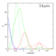
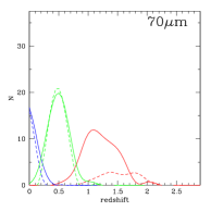
Fig. 5 demonstrates these model differences explicitly, demonstrating that many more sources are detected in the extremes of the temperature distributions in the $\Phi$(${\cal L}$, ${\cal C}$)  model. Moreover, the predicted distributions are often radically different in form in the $\Phi$(${\cal L}$, ${\cal C}$)  case. The double peaked profile apparent in the redshift distributions presented in Figure 2 is a result of temperature differences in the underlying IR population. Fig. 5, therefore, illustrates the strongest differences between the univariate and bivariate models.

Recently deep counts at 24$\mu m$, 70$\mu m$ and 160$\mu m$, obtained with the MIPS intrument on Spitzer, have become available (e.g. Dole et al. 2004; Papovich et al. 2004). This presents further opportunities to test the efficacy of the bivariate model. Figure 6 presents the bivariate model prediction for the Spitzer MIPS bands with the observed counts overlaid. Generally, the observed trends are reproduced, but discrepancies are apparent, most notably a deficit in the Spitzer counts between 1mJy - 10mJy. Addressing these discrepancies is beyond the scope of this present work and will be reserved for further study.

4. Studying the submillimeter galaxies

Spitzer data is just beginning to be transmitted back to Earth, and analysis and spectroscopic followup will take a significant effort. Detailed comparison of our models with the Spitzer sources will be the focus of an upcoming paper, once an initial census of the Spitzer surveys are complete. However our understanding of the deepest 850$\,\mu$m  submm sources has recently reached a relatively mature state, with the measurement of spectroscopic redshifts for a large sample (Chapman et al.  2003b; Chapman et al. in preparation). In this section, we compare our predictions for the submm galaxies (SMGs) directly with the measurements.

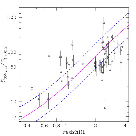
The S_850μm/S_1.4GHz  ratio provides a measure of the degenerate quantity (1+$z$)/T_d (Blain 1999b), coupled with any evolution in the Far-IR/radio correlation. As the redshift parameter has now been independently measured for the SMGs, we can directly compare the S_850μm/S_1.4GHz predictions of our model to the SMGs. Fig. 7 shows the S_850μm/S_1.4GHzindices for SMGs with redshifts, compared to our model prediction. Note that the model includes only the range of dust temperatures observed locally in the IRAS population, whereas a variation in the radio to farIR ratio likely increases the scatter further.

The actual submm population appears to span a larger range than the local IRAS galaxy population, although there are some caveats to consider. The SMG surveys are missing cold sources in the radio detection criterion, and thus there is some asymmetry in the actual observations towards hotter dust temperatures. At low redshifts, there are some apparently very cold galaxies, which are not predicted by the local IRAS extrapolation. If the SMG identifications are correct, they may signal a rare population which has no local analogs.

A remaining question is the interpretation of sources in our model. Ongoing debates discuss whether accretion power from super-massive black holes or bursts of star formation is heating the dust in ULIRGs. Our model has not assumed either explicitly. Rather, we have taken the distribution of 60$\,\mu$m/100$\,\mu$m color found locally in the IRAS galaxy population and assumed it describes galaxies at all redshifts. However, AGN are known to typically have warmer colors, and our model may not accurately reflect their possibly larger contributions at higher redshift, higher luminosity.

A test for AGN contribution is whether the SMGs are unusually bright in the X-ray, where even obscured AGN should reveal themselves, penetrating high columns of gas. The radio identification of the submillimeter sources has allowed their location to be pinpointed. In Barger et al. (2001a,b), it was pointed out that approximately 10% of the X-ray sources were submillimeter  detected in the Chandra Msec exposure centered on the HDF. The 2 Msec exposure in this field has detected the majority ($\sim$ 90%) of the radio-SMGs (Alexander et al. 2003). As this radio identified submillimeter population represents $\sim$65% of the total blank-field SCUBA population at $S_{\rm 850\mu m}$$>$5 mJy, this implies a fraction $>60$% of the total SCUBA population is detectable in a 2 Msec Chandra exposure. The typical inferred star formation rate from this analysis is roughly 1000${\rm\,M_{\odot}\,yr^{-1}}$, similar to that deduced from the submillimeter luminosities.

The sources with considerably higher X-ray luminosities, where the X-ray implied SFR would severely exceed the submillimeter estimate, suggest an AGN must be generating the X-ray emission, and we emphasize that our model does not account for such sources explicitly. Note however that in Fig. 7, only one source explicitly stands out from the distribution due to radio excess over the model expectations.

Let us now look specifically at the differences between the bivariate and single variable models. The counts and redshift distributions are natural measurable outputs from our model. The univariate model predicts a one-to-one mapping of S_850μm/S_1.4GHz with redshift [for a fixed Q-value (Helou et al. 1985)]; clearly the observed scatter seen in Figure 7 cannot be explained such a simple mapping. The bivariate model naturally introduces a scatter into this relationship, and the dashed lines in Figure 7 correspond to the 1$\sigma$ width of the S_850μm/S_1.4GHz distribution as a function of redshift. It is a straw man argument to compare a single SED model to our data, which provides an unphysically narrow range of submm/radio colors (e.g., C02). A more realistic approach is to constrain the width of the color distribution of our best fitting bivariate model until there is only a single temperature SED associated with a given luminosity. This single variable model can be thought of as mapping the dust temperature monotonically to the source luminosity.

We first extract the counts from our models and compare directly with the measured field counts. Both models are able to fit the counts well within current measurement errors. The submm counts are insensitive to the width in color, ${\cal C^{\prime}}$, in our model due to the degeneracy in T_d versus redshift. Therefore neither of these models is better constrained by the submm counts. The far-IR background (Puget et al.  1996; Fixsen et al. 1998) also provides little constraint on the detailed form of the high-$z$ evolution, requiring only that the evolution function fall off quickly enough at high redshifts to avoid generating too high an energy density. Both models generate submm and far-IR background values midway between the measurements of Puget and Fixsen. The model is therefore self-consistent as a generalization to the evolution of the entire submm population. While the model does not provide a unique description of the submm galaxies, it is physically motivated by the detailed properties of local and moderate redshift IRAS galaxies.

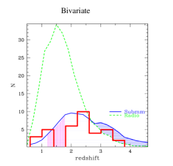
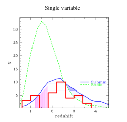
We can use our model to predict the redshift distributions for radio (1.4 GHz) and submm (850$\,\mu$m) galaxies. In Fig. 8, we show the prediction for the bivariate model (left panel) compared to the single variable LF model (right panel). The bivariate scenario marks a difference in the predicted N($z$), where a deficit of sources at the redshift peak are seen relative to the single variable model, with a corresponding boost to the higher redshift sources. This behavior was described in C02, where the far-IR/radio distribution provides a similar effect. The shaded regions between the radio and submm model curves reveal the submm sources which are not expected to be detectable in the radio. In the bivariate model, a range of hotter dust temperatures for a given luminosity lead to a higher redshift range for radio detectability. While not statistically significant, the bivariate models appears to follow the observed redshift distribution.

Understanding of the full redshift distribution for the submm population through deep optical and millimeter spectroscopy will provide a strong test of these models and the applicability of the local bivariate ${\cal L}-{\cal T}$ relation to this high redshift population. The discovery of the redshift distribution for the radio detected submm galaxies (Chapman et al. 2003a,c) is shown overlaid on our models in Fig. 8. A remarkable agreement is found between the data and our model, with a preference for the flattened distribution and expanded range of redshifts in the bivariate picture. We conclude that submm galaxies exhibit at least as large a range in dust temperatures as local IRAS galaxies, and likely a larger range.