A Survey of O vi Absorption in the Local Interstellar Medium

Abstract

We report the results of a survey of O vi $\lambda$1032 absorption along the lines of sight to 25 white dwarfs in the local interstellar medium (LISM) obtained with the Far Ultraviolet Spectroscopic Explorer (FUSE). We find that interstellar O vi absorption along all sightlines is generally weak, and in a number of cases, completely absent. No O vi absorption was detected with significance greater than 2 $\sigma$ for 12 of the 25 stars, where the 1 $\sigma$ uncertainty is $\sim 4$ mÅ, equivalent to an O vi column density of $\sim 3\times 10^{12}$ cm^-2. Of the remaining stars, most have column densities N(O vi)$<10^{13}$ cm^-2 and no column densities exceed $1.7\times 10^{13}$ cm^-2. For lines of sight to hot (T${}_{\rm{eff}}>40,000$ K) white dwarfs, there is some evidence that the O vi absorption may be at least partially photospheric or circumstellar in origin. We interpret the “patchy” distribution of O vi absorption in terms of a model where O vi is formed in evaporative interfaces between cool clouds and the hot, diffuse gas in the Local Bubble (LB). If the clouds contain tangled or tangential magnetic fields, then thermal conduction will be quenched over most of the cloud surface, and O vi will be formed only in local “patches” where conduction is allowed to operate. We find an average O vi space density in the LISM of $2.4\times 10^{-8}$ cm^-3, which is similar to, or slightly larger than, the value in the Galactic disk over kpc scales. This local density implies an average O vi column density of $\sim 7\times 10^{12}$ cm^-2 over a path length of 100 pc within the LB. The O vi data presented here appears to be inconsistent with the model proposed by Breitschwerdt & Schmutzler (1994), in which highly ionized gas at low kinetic temperature ($\sim 50,000$ K) permeates the LB. Our survey results are consistent with the supernova-driven cavity picture of Cox & Smith (1974) for the LB, and in particular, the recent model by Cox & Helenius (2003) for the creation of cool clouds in the LB by magnetic flux tubes, and their subsequent magnetic shielding from conduction.

1 Introduction

It has now been several decades since two important observations revolutionized our understanding of the structure and ionization of the interstellar medium (ISM). The first was the discovery (Bowyer, Field & Mack, 1968) and subsequent investigation (McCammon et al., 1983) of the 0.25 keV soft X-ray diffuse background, which implied that a substantial fraction of the Galactic disk in the solar neighborhood was occupied by low density, hot ($T\gtrsim 10^{6}$ K) gas. The second was the discovery of O vi absorption lines arising in the ISM (Rogerson et al., 1973; York, 1974; Jenkins & Meloy, 1974; Jenkins, 1978a). With an ionization potential of 114 eV, O vi is very difficult to produce by photoionization. In addition, the observed O vi line profiles are broader than interstellar lines of lower ionization potential. Consequently, the O vi ionization was most naturally explained by collisional ionization in a hot gas ($T\gtrsim 2\times 10^{5}$ K). The O vi line profiles have widths consistent with thermal broadening from such a hot gas.

On the theoretical side, Cox & Smith (1974) studied the role of supernova explosions in creating large, low-density cavities of hot gas in the ISM. McKee & Ostriker (1977) provided a self-consistent theory of the ISM in which warm ($T\sim 10^{4}$ K) ionized clouds exist in this hot gas. The McKee & Ostriker (1977) model attempted to explain the pressure of interstellar clouds, the soft X-ray background, the O vi absorption, and the ionization and velocities of the clouds. Although numerous theoretical models have since been proposed which emphasize the roles of magnetic fields, or different values for the filling factor of the hot gas (Slavin & Cox, 1992), the general picture of a turbulent, three-phase ISM which is churned up by supernovae has endured. Much recent progress has been made in developing multi-dimensional magneto-hydrodynamic simulations of the ISM (Avillez, 2000; Avillez & Breitschwerdt, 2004), which show the growth of structures both large and small due to shocks, radiative cooling, and thermal instabilities.

The origin of the O vi absorption has been the subject of much debate and modeling. The most widely held view is that the O vi is formed in conductive interfaces between the hot, $10^{6}$ K gas and cool embedded clouds (McKee & Ostriker, 1977; Cowie et al., 1979). This explanation is consistent with a number of characteristics of the O vi absorption, such as their line widths and kinematics. Jenkins (1978b) has shown that the rms dispersion in O vi components is only $\sim 26$ km s^-1. This narrow velocity spread seems incompatible with formation in turbulent, expanding supernova remnants. Furthermore, Cowie et al. (1979) have shown that there is a correlation between the kinematics of the O vi absorption and UV lines from lower ionization lines, implying a physical correlation between the hot and cool gas. Finally, models of the conductive interfaces predict column densities of O vi which are in general agreement with observations (Slavin, 1989; Borkowski et al., 1990).

Despite these successes, alternative models have received a lot of attention. Cox & Smith (1974), Slavin & Cox (1992) and Shelton (1998) have investigated the production of O vi in the interior of bubbles carved out in the ISM by supernova explosions. Slavin & Cox (1992) have modeled the evolution of supernova remnants, including non-equilibrium effects and magnetic fields. They find that hot gas inside the bubble condenses onto the interior shell wall, and will have significant column densities of O vi. At later times in the remnant evolution ($\sim 3\times 10^{6}$ yr), there is considerable cooling inside the bubble, and large amounts of O vi are produced in the middle of the bubble. In these later phases of the bubble evolution, expansion has ceased and consequently the O vi line widths would be much narrower than in the turbulent expanding phase (Shelton, 1998). Averaged over the bubble lifetime, Slavin & Cox (1992) predict the most probable value of the O vi column density from one crossing of the bubble wall to be $4.5\times 10^{13}$ cm^-2, which is higher than observed.

Comparisons of models with observation have been hampered by the necessarily complicated sight lines observed with Copernicus, the only far-ultraviolet spectrograph prior to the Far Ultraviolet Spectroscopic Explorer (FUSE) with high enough spectral resolution to study O vi absorption. Due to its low effective area, however, Copernicus could only observe bright, early-type stars that are, with a few exceptions, at distances exceeding 100 pc from the Sun. Shelton & Cox (1994) reanalyzed the Copernicus data and showed that a significant fraction of the O vi column density along most distant lines of sight was contributed by a region of hot gas surrounding the Sun called the Local Bubble (LB). However, the Copernicus data did not allow the determination of where in the LB the O vi was formed; i.e. on conductive interfaces or in condensation regions at the bubble wall. The much higher sensitivity of FUSE permits observation of nearby white dwarfs, where the problem of averaging and blending of many different physical conditions along the line of sight are minimized, allowing the study of the distribution of O vi in the LB. A separate study of low-ionization species in the LISM has been carried out by Lehner et al. (2003) using many of the same lines of sight as the present study.

1.1 The Local Interstellar Medium

The Sun lies inside a low density, warm cloud ($n\sim 0.1$ cm^-3, $T\sim 7000$ K) which extends $1-10$ pc from the Sun (Lallement & Bertin, 1992; Lallement, 1995). The Sun is located near the edge of this local interstellar cloud (LIC) (Linsky et al., 2000), which is immersed inside a hot ($T=10^{6}$ K), very low density ($n\sim 0.005$ cm^-3) cavity called the Local Bubble (Cox & Reynolds, 1987). Although it is unclear how representative the LB is of other regions within our Galaxy, it provides a unique local laboratory for studying the formation of O vi in either diffuse hot gas or in conductive interfaces to cool clouds. Within the LB, there are numerous clouds of low column density, although the volume filling factor of clouds is quite small. In addition to the LIC, Lallement & Bertin (1992) have identified the G cloud, and Linsky et al. (2000) have provided evidence for two additional clouds that they dub the North and South Galactic Pole clouds. Gry et al. (1995) have identified six clouds along the line of sight to $\epsilon$ CMa, which is 132 pc distant. Ferlet (1999) has estimated that the LB could contain more than 2000 diffuse clouds. Therefore, lines of sight to nearby ($50-100$ pc) white dwarfs should pass through a minimum of one cloud interface (the LIC), and will likely intercept several clouds. Ferlet (1999) notes that most stars within only 20 pc of the Sun exhibit two or three absorption components in Ca ii.

It has been assumed that the LB is full of million degree gas because of the observed emission of soft x-rays (Snowden et al., 1998). The exact origin of the LB is not known, although it is presumably due to one or more supernova explosions. Maiz-Apellaniz (2001) and Frisch (1998) have presented kinematical evidence that subgroups of stars in the Sco-Cen OB assocation passed through the current boundary of the LB about 5 million years ago, and OB stars in these subgroups provided the supernovae that created the LB. Berghöfer & Breitschwerdt (2002) arrive at similar conclusions from a study of the trajectories of moving stellar groups in the solar neighborhood, concluding that the Local Bubble was created by up to 20 supernovae in the past $10-20$ Myr. Smith & Cox (2001) also suggested that supernova explosions in the Sco-Cen region could have resulted in runaway OB stars that passed close to our Sun. A sequence of about 3 supernovae over a few million year period from these runaway stars could provide the energetics to power the LB.

Cox (1998) suggested that a substantial amount of the soft x-ray background might be due to charge transfer of heavy solar wind ions with interstellar neutrals in the heliosphere (in a process analogous to the proposed explanation of x-ray emission from comets by Cravens (2000)). This process would lead to time-dependent x-ray emission due to fluctuations in the solar wind. Indeed, Snowden et al. (1994, 1998) has reported time-variable “long-term enhancements” of order 30% in the two lowest energy bins in the ROSAT/PSPC x-ray background. Current estimates of the contribution of this process to the soft x-ray background range from $\sim 25$% (Snowden, 2004) to $\sim 25-50$% (Robertson et al., 2001).

Vallerga (1996) used EUVE data to show that He is more ionized than H in the LISM. In subsequent work, Vallerga (1998) argued that stellar EUV sources are not capable of providing the observed He ionization level. Slavin & Frisch (2002) have modeled the soft x-ray radiation field within the LB near the Sun as a combination of three sources: (1) radiation from nearby B stars and white dwarfs, (2) emission from a $10^{6}$ K gas in collisional ionization equilibrium, and (3) radiation from an evaporative interface at the boundary of the LIC. This model successfully explains a number of observations, such as the ionization of He and H, and the ionization ratios of Mg i to Mg ii and C ii* to C ii towards $\epsilon$ CMa. Furthermore, in order to match the observations toward $\epsilon$ CMa, an EUV radiation field larger than that from nearby stars plus diffuse emission from the hot gas in the LB was required, providing indirect evidence for an evaportive boundary around the LIC. The existence of this evaporative boundary could be tested through observations of O vi towards nearby stars.

Breitschwerdt & Schmutzler (1994) proposed an innovative model for the soft X-ray background in which supernovae drive an adiabatic expansion of hot gas. The gas cools quickly as it expands, and highly ionized stages are “frozen in” to the gas. The soft X-ray emission is due to delayed recombination at low kinetic temperatures ($\sim 4\times 10^{4}$ K). In this model, a significant amount of O vi is also produced in wide-spread, highly excited gas within the supernova remnant. One of the successes of this model is its natural explanation of how cool clouds can survive inside the LB. If the LB contained million degree gas, then conduction at cloud surfaces would evaporate the clouds in a relatively short time. The existence of cool clouds in the LB implies that either the ambient medium is cool, that conduction is inoperative, or cool clouds are being replenished. We note that Shelton (2003) has recently shown that the $\sim 2\sigma$ upper limit on the intensity of observed O vi emission from a null detection along one line of sight in the LB is about twice the intensity expected from this model.

Hurwitz et al. (2004) report that a spectrum of the LB obtained with the Cosmic Hot Interstellar Plasma Spectrometer (CHIPS) indicates that the diffuse EUV emission is much fainter than that predicted from a $10^{6}$ K gas in collisional ionization equilibrium, as predicted by the soft-xray observations. The emission measure of the Fe ix 171 Å line is an order of magnitude less than predicted, and the emission lines of Fe x – Fe xii were not detected at all, even though they would be expected to have similar intensities. Depletion of iron in the LISM and/or foreground absorption could explain the low intensity of the Fe ix emission, but not the absence of the Fe x line. Other possible explanations for unexpectedly low EUV emission include non-equilibrium ionization and solar wind charge exchange effects.

Cox & Helenius (2003) have proposed a model for the origin of the diffuse clouds in the Local Bubble, in which a magnetic flux tube anchored at two points on opposite sides of the LB pulls free of the boundary wall and, through its own tension, is pulled to the center of the bubble. The authors have investigated the dynamics of this flux tube, and they conclude that a converging flow of matter occurs in the tube, and leads to the formation of one or more clouds near the center of the bubble.

A thorough review of the LISM is not possible in this paper, and we have just touched on subjects relevant to our survey of O vi absorption. The interested reader is referred to a recent review article on Local Bubble research by Breitschwerdt & Cox (2004) for a more extensive discussion.

In the next section, we describe our survey of O vi absorption toward white dwarf stars within and near the LB, report the measurements and their uncertainties. In the following sections, we discuss the implications of these results in terms of the models discussed above.

2 Observations and Results

2.1 The Survey Sample

In this paper, we report observations of 29 nearby white dwarfs obtained with the FUSE. Observations used in this survey were obtained for a variety of purposes (photometric calibration, deuterium snapshot survey, etc), and hence the survey data are not homogeneous in terms of signal-to-noise. In the second year of FUSE observations, we added white dwarfs to the Guaranteed Time Observer’s target list (program P204) in order to provide even sky coverage. DA white dwarfs with surface temperatures less than 40,000 K are the preferred targets, since most of them have essentially pure hydrogen atmospheres, although it should be noted that some percentage of DA white dwarfs with effective temperatures less than 50,000 K contain detectable metals (Barstow et al., 2003). DA white dwarfs hotter than 40,000 K can contain elements heavier than H or He, such as C, N, O, Si, P, S, Fe, and Ni in their photospheres, giving rise to stellar absorption lines (Vennes & Lanz, 2001; Barstow et al., 2003). Unlike rapidly rotating, early-type stars that are typically used as background sources to study interstellar absorption lines, the photospheric lines of white dwarfs are not significantly rotationally broadened and can be easily confused with interstellar or circumstellar features, especially if the radial velocity of the star is unknown or is the same as the interstellar velocity. Nevertheless, white dwarf spectra generally have fairly smooth continua making them excellent background sources for studying the interstellar medium.

The 29 white dwarfs observed in this survey of the LISM are listed in Table 1, along with their distances, H i column densities, Galactic coordinates, spectral types, effective temperatures, and FUSE dataset names. The positions of the survey stars in Table 1 are plotted in Figures 1 and 2, projected onto the Galactic and Meridional planes, respectively. In these figures, we have plotted only the 25 stars without strong stellar O vi contamination, as described in Section 2.2 below. In Figure 1, only the subset of these 25 stars with $|b|<35^{\circ}$ are displayed, to avoid misleading projection effects. Overlayed in Figures 1 and 2 are the main boundaries of the 20 mÅ Na i D2 equivalent width contours from Lallement et al. (2003), which define the Local Cavity. A Na D2 line equivalent width of 20 mÅ corresponds to an H i column density of $\log N$(H i)$=19.3$. This contour level marks the beginning of a steep rise in density; essentially defining an H i “wall” surrounding the local cavity. Also shown in both figures is the contour map of the hot LB, as defined by the 0.25 keV soft x-ray emission (Snowden et al., 1998).

Considerable uncertainty exists in the distances to the white dwarfs and in the location of the hot LB contour from the soft x-ray emission. Only two stars in our survey have parallaxes listed in the Hipparcos catalog (Perryman et al., 1997) – WD 0501$+$527 and WD 1314$+$293. However, even in these cases, the uncertainties are not small – the parallax error is 21% for WD 0501$+$527 and 27% for WD 1314$+$293. Even more worrisome is the fact that the Hipparcos-determined distance of 32 pc to WD 1314$+$293 disagrees with numerous other determinations that all indicate a distance of about 65 pc. Kruk et al. (2002) have discussed this in detail, and we have adopted their assumed distance of $68\pm 13$ pc. The distances to the remaining stars in Table 1 are taken from Vennes et al. (1997) and Holberg, Barstow & Sion (1998), who employ photometric techniques to derive distances. The star’s spectral energy distribution is used to determine the effective temperature and gravity of the star, and these atmospheric parameters are used in conjunction with theoretical evolutionary sequences to determine the star’s radius, and hence its absolute magnitude. The distance is then determined from the star’s apparent magnitude. Even though white dwarfs have well understood spectra, the resultant uncertainty in distance is still $\sim 25-30$%.

There is also significant uncertainty in the radial extent of the hot LB as determined from soft x-ray emission. In order to determine the scaling relation between soft x-ray emission and distance, (Snowden et al., 1998) used a distance of $65\pm 5$ pc to the molecular cloud complex MBM 12 as determined from ISM absorption line measurements (Hobbs, Blitz & Magnani, 1986) together with X-ray shadowing measurements (Snowden, McCammon & Verter, 1993). This distance determination is a matter of some dispute, and the true distance may be considerably larger than this (Luhman, 2001; Andersson et al., 2002). We conclude that the LB may extend all the way out to the boundary of the cavity demarked by the Na i contours.

Lehner et al. (2003) points out that in the face of distance uncertainties, it is also useful to consider the H i column densities along the lines of sight to the target stars. Objects with column densities $\lesssim 19.0$ dex are within the LB, while objects with $19.0\lesssim$ logN(H i) $\lesssim 19.3$ are probably very near the bubble wall, and stars with logN(H i) $>19.3$ are beyond the LB wall. In our sample of 25 white dwarfs, 8 objects have logN(H i) $\gtrsim 19.0$ (see Table 1).

2.2 FUSE Data

Moos et al. (2000) and Sahnow et al. (2000) have provided an overview of the FUSE spectrograph and its on-orbit performance. In brief, the FUSE instrument consists of two telescopes, each of which has two channels optimized for specific wavelength ranges. The SiC channels cover the wavelength range 905-1104 Å, while the LiF channels cover the 990-1185 Å region. Hence, the O vi $\lambda$1032 line is covered by both the SiC and LiF channels on sides 1 and 2 of the instrument. Spectra of O vi are obtained in channels LiF1, LiF2, SiC1 and SiC2. The SiC channels have only about one-third the sensitivity of the LiF1 channel, and the LiF2 channel is $\sim 60$% as sensitive as LiF1 at 1032 Å. Since the O vi line is weak, the best data is usually obtained in the LiF1 channel. Furthermore, in many of the observations obtained early in the FUSE mission, the channels were not properly aligned, and hence for some datasets, the target was not in the aperture of the SiC channels. The target was always in the LiF1 channel, since this channel contains the guide camera. Neverthless, we have used data from all channels if the signal-to-noise is adequate.

Some of the observations were taken in the MDRS (4 arcsec) and HIRS (1.5 arcsec) spectrograph apertures, although most of the data were obtained in the LWRS (30 arcsec) aperture. A typical observation consisted of $10-20$ exposures, each of which was $\sim 10$ minutes in duration, yielding total integration times of $5-10$ ksec per target. All data for these stars were reprocessed with version 1.8.7 of the CALFUSE data reduction pipeline.

The spectra produced by the FUSE concave gratings are astigmatic, with significant curvature present in the two-dimensional point spread functions. However, the O vi lines lie near one of two astigmatic correction points, where the curvature cannot be easily removed. Hence, spectral extractions were performed by simply collapsing the two-dimensional spectra to one-dimension. The resulting spectral resolution is $\sim 15,000$ (FWHM) with no appreciable difference between the MDRS and LWRS aperture data (the point spread function is much smaller than the width of either aperture).

There are two sources of spectral motion in the FUSE instrument that can degrade spectral resolution: motions of the primary mirrors, and rotation of the gratings in each spectrograph channel. Shifts during an exposure are typically only $0.01$ Å. Consequently, prior to coadding all the exposures in a given observation, the spectra were registered using the C ii $\lambda$1036 line as a reference.

At the present time, no correction for fixed pattern noise in the detectors is available. A typical resolution element at 1032 Å covers $\sim 100$ detector pixels (10 pixels in the dispersion direction and 10 pixels of astigmatic height), which smooths out some of the pixel-to-pixel flat field irregularities. For those spectra whose exposures had some movement, the shift-and-add coaddition process serves to further wash out some of the fixed pattern noise in the spectra from each channel. Whenever possible, we combined spectra for a given star from all channels and all observations with weights inversely proportional to the noise variances. Since the different channels are recorded on different regions of the detector, this further mitigated the effect of fixed pattern noise. Beginning in the second year of FUSE observations, we began to take data in a special mode in an attempt to mitigate fixed pattern noise. When observing in the LWRS aperture, the target was observed at several different locations within $\pm 10$ arcsec of the aperture center, resulting in spectra at different locations on the detector. Many, but not all, of the observations with program ID P204 (see Table 1) were obtained in this manner.

Typical signal-to-noise ratios in the final coadded spectra are $\sim 20$ to 50 per resolution element at 1032 Å. Nevertheless, some fixed pattern noise remains in the data, and this serves to limit our ability to measure weak absorption features.

Barstow et al. (2001, 2002) and Wolff et al. (2001) have reported detection of stellar O vi lines in the FUSE spectra of the hot (T${}_{\rm{eff}}\gtrsim$ 60,000 K) white dwarfs PG 1342$+$444, RE J0558$-$371 and Feige 55. One surprising discovery from this survey was the existence of strong photospheric O vi lines in the spectra of two white dwarfs with effective temperatures below 50,000 K: WD 0131$-$163 and WD 2156$-$546 (see Fig 3). Stellar O vi lines are also evident in the spectra of the white dwarf in the close binary WD 2013$+$400 and the hot helium-rich white dwarf WD 0501$-$289. These stars all display a strong O vi 1038 Å line, with a 1032/1038 doublet ratio of approximately unity, indicating that the lines are optically thick. The photospheric nature of the strong O vi lines in these stars is confirmed by comparing the O vi radial velocities to those of other photospheric lines. We have eliminated these stars from further consideration in this survey, since an accurate measurement of interstellar O vi is not possible.

There are several other features to note in Figure 3 that are the same for all the white dwarf spectra. First, interstellar C ii $\lambda$1036 and O i $\lambda$1039 absorption lines are present. In most of the spectra in our survey, the C ii $\lambda$1036 line is lightly saturated with a full width half maximum (FWHM) of $\sim 100$ mÅ. In low column density lines of sight, such as HZ 43, the C ii $\lambda$1036 and O i $\lambda$1039 FWHM are $\sim 17$ km s^-1, representing the limiting resolution of the instrument at these wavelengths. C ii* $\lambda$1037 interstellar absorption is also present if the electron density is high enough somewhere along the line of sight. Finally, we note the absence of H₂ absorption, which is a ubiquitous feature in far-UV spectra along more distant Galactic sightlines, in all but 3 of our survey stars. Lehner et al. (2003) reports total column densities of $\log$ N(H₂) $\sim 14.5-15$ towards WD 0004$+$330, WD 1636$+$351, and WD 1800$+$685. Simply assuming an HD/H₂ ratio equal to the observed local D/H ratio of $1.5\times 10^{-5}$ (Linsky, 1998; Moos et al., 2002), would then imply an HD column density of $\log N({\rm HD})<1.5\times 10^{10}$ cm^-2. However, Watson (1973) has pointed out that ion molecule, isotope exchange reactions in the ISM can form HD preferentially in comparison to H₂, with enhancements of order of $\sim 100$. Even if one assumes such a large enhancement of HD, we predict that the resulting equivalent width of the 6-0 R(0) Lyman transition of HD at 1031.909 Å would be $<0.25$ mÅ. Hence, this HD line is not expected to contaminate the $\lambda$1032 line of O vi in the LISM.

2.3 O vi Measurements

The zero point of the wavelength scale for calibrated FUSE spectra taken in the LWRS aperture is uncertain by $\sim 15$ km s^-1, due to uncertainty in the location of the star in the aperture, arising from relative uncertainties of celestial coordinates of the target stars with respect to guide stars (especially due to proper motion). Consequently, we have used the C ii $\lambda$1036.336 line to set the zero point for the interstellar cloud velocity along each line of sight. An additional check of the C ii $\lambda$1036 line was provided by the interstellar O i $\lambda$1039.23 line. A number of the white dwarfs in our survey also displayed photospheric P iv absorption lines at 1030.515 and 1035.516 Å, which were used in conjunction with published stellar velocities (Holberg, Barstow & Sion, 1998) to check the dispersion solution in the region 1030-1039 Å. Based on these interstellar and stellar lines, we are confident that our corrected wavelength scale at 1032 Å is accurate to $<10$ km s^-1. Spectra of the 25 white dwarfs, after excluding the ones noted above as having strong stellar O vi contamination, are shown in Figure 4. These spectra have been normalized to the continuum, and only the region near the O vi $\lambda$1032 line is shown. The O vi absorption line is remarkably weak in all sightlines. Since the O vi $\lambda$1031.93 line has an f-value twice as large as the 1037.62 Å member of the doublet, we have measured only the 1032 Å line equivalent widths. After some experimentation, a velocity integration range of $\pm 40$ km s^-1 was chosen in order to be large enough to fully cover the expected thermal width of an O vi line at $T=200,000$ K, plus some margin for wavelength calibration uncertainties and real velocity offsets, but also narrow enough to exclude nearby stellar features.

The measured equivalent widths and column densities are given in Table 2. The column densities are derived from the measured equivalent widths, assuming a linear curve of growth. The uncertainties in the measured equivalent widths were determined empirically from the following considerations. In addition to fixed pattern noise, there is also the likelihood that weak photospheric absorption lines from various metals could be present in the spectra. We have decided to treat these lines as just another source of noise. Hence, we measured the equivalent width in numerous regions of the spectra near the O vi line where we did not expect to find any stellar or interstellar lines; i.e., where the expected equivalent width would be zero. The standard deviation in the measured equivalent widths was then used as our empirically determined uncertainty. Consequently, the uncertainties in the equivalent widths in Table 2 combine systematic and random errors.

No O vi absorption was detected with significance greater than 2 $\sigma$ for 12 of the 25 stars. As can be seen from Table 2, a typical 1 $\sigma$ uncertainty is $\sim 4$ mÅ (equivalent to an O vi column density of $\sim 3\times 10^{12}$ cm^-2). Of the remaining stars, most have column densities N(O vi)$<10^{13}$ cm^-2 and no column densities exceed $1.7\times 10^{13}$ cm^-2.

2.4 Photospheric and Circumstellar Contamination

We now return to the issue of photospheric contamination of the O vi interstellar lines. As mentioned above, O vi lines can be formed in the atmospheres of hot white dwarfs, even if they have relatively low metallicity. It was easy to reject the obvious cases where the photospheric O vi was strong and present in both members of the O vi 1032/1038 doublet. But, what, might we ask, is the potential for contamination by weak stellar O vi lines? We have computed NLTE photospheric models of white dwarfs for a grid of effective temperatures and atmospheric abundances assuming $\log g=8$ and a homogeneous H$+$O chemical composition. The results are illustrated in Figure 5. The models indicate that stars with T${}_{\rm{eff}}<40,000$ K should not have any appreciable absorption by O vi. Hence, the cool stars WD 0050$-$332, WD 0549$+$158, WD 1017$-$138, WD 1254$+$223, WD 1615$-$154, WD 1636$+$351, WD 1845$+$019, WD 1847$-$223, and WD 2111$+$498 should not show photospheric O vi lines. Above this temperature, stars with low abundances can have weak stellar absorption lines with strengths of a few mÅ rising to $\sim 10$ mÅ for T${}_{\rm{eff}}=60,000$ K and log(O/H)$<-7$. In Figure 6, we show the data for 5 of our survey stars, overlayed with photospheric models. In these models, the abundances of O, P and Fe were adjusted to give the best fits to the data. In the cases of P and Fe, there were multiple lines with different strengths available for the fit; however, in the case of oxygen, there is only the 1032/1038 doublet. Typically, the best fitting models have log(O/H)$\approx-8$. In the case where the stellar radial velocity and the interstellar velocity are quite different, there is no ambiguity as to whether a line is stellar or interstellar. For instance, as shown in the top panel of Figure 6, the stellar O vi line in WD 0455$-$282 is distinctly offset from the broad, presumably interstellar O vi line. However, in cases where the stellar radial velocity is unknown (which, sadly, is the majority of the cases), there is a general uncertainty as to the level of contamination of the observed O vi line by the star’s photosphere for stars hotter than 40,000 K.

Consequently, for the hotter stars, our O vi  measurements can be viewed as providing upper limits to the interstellar absorption, since some photospheric contribution may be present depending on the abundance of oxygen in the star. For the models shown in Figure 6, the equivalent width of O vi reported for WD 0455$-$282 appears to not be contaminated. Also, for WD 2111$+$498, the Fe iii $\lambda$1032.12 line does not affect our measurement of O vi, since it is outside our 40 km s^-1 measurement window. Note also that this star has an effective temperature well below 40,000 K, so no photospheric O vi is predicted. For the other three stars in Figure 6, it is possible to produce photospheric models that can explain a significant part of the observed O vi absorption. We find that after subtracting our best fitting photospheric model, that the interstellar O vi  equivalent widths for WD 0501$+$527, WD 2211$-$495 and WD 2331$-$475 are 1.3, 5.6 and 5.4 mÅ, significantly lower than the measured values of 4.4, 16.4, and 13.1 mÅ, respectively. These model-dependent corrected values are noted in the footnotes to Table 2. At this point there is no satisfying model for explaining why the photospheric O vi abundances that we have measured are much smaller than the O iv and O v abundances measured by Vennes & Lanz (2001) and Barstow et al. (2003). Vennes & Lanz (2001) suggested that this difference may be the result of a steep oxygen abundance gradient that increases with decreasing optical depths. Consequently, we have assumed throughout the rest of this paper that the measured column densities toward these stars are formed in the ISM.

The O vi line velocities reported in Table 2 are measured with respect to the C ii $\lambda$1036 line, which we use as the low ionization ISM cloud velocity. In this frame of reference, the O vi line velocity is $\lesssim 20$ km s^-1 for most lines of sight. The O vi absorption along the line of sight to WD0455$-$282, at $\sim-35$ km s^-1, is a notable exception. The line of sight to this star appears more complicated than others in the LISM. The C ii $\lambda$1036 interstellar line has multiple components; the strong central one at 0 km s^-1 (by definition) and another reasonably strong line at $-54$ km s^-1. The stellar lines in the FUSE spectrum are at $\sim+60$ km s^-1 relative to the central C ii ISM line, in good agreement with the velocities of stellar and interstellar lines reported by Holberg, Barstow & Sion (1998) from IUE observations. Holberg, Barstow & Sion (1998) also report the presence of Si iv and C iv absorption lines blueshifted by $-53$ km s^-1 with respect to the stellar photosphere, which they cite as evidence for mass loss from this hot, DA white dwarf. We do not observe O vi at this velocity. We will thus assume that the O vi line, which appears to have multiple unresolved components, is interstellar in nature.

2.5 Line Widths

In order to quantify the widths of the O vi absorption lines, we have computed their mean absolute deviations in order to avoid the effects of noise in the wings of the line profile. The average absolute deviation about the mean is defined as $v_{mad}={\sum_{i}f_{i}|v_{i}-\overline{v}|}/\sum_{i}f_{i}$, where $f_{i}$ is the residual intensity and $\overline{v}$ is the line velocity centroid. The results are given in Table 2 for those lines of sight having sufficient O vi line strengths and signal-to-noise to permit a measurement. The average value of $v_{mad}$ is $16\pm 2$ km s^-1. For a normal distribution, the standard deviation is $1.25v_{mad}$, or 20 km s^-1. This observed line width should be compared with the expected width, $\sigma_{tot}$, of an oxygen line formed in a $T=3\times 10^{5}$ K gas, having a thermal width of $\sigma_{t}=\sqrt{kT/16m_{p}}$ convolved with the FUSE line spread function, $\sigma_{lsf}\sim 8.5$ km s^-1. The expected line width is then $\sigma_{tot}=\sqrt{\sigma_{t}^{2}+\sigma_{lsf}^{2}}=15$ km s^-1, which is less than our observed linewidths in the LISM. This should be compared with the results of Jenkins (1978b), who found $\sigma_{tot}\sim 26$ km s^-1 over much longer pathlengths in the Galactic disk.

3 Discussion

The weakness of O vi absorption, not to mention its total absence along many sightlines, in the LISM has important implications for models of the Local Bubble, as well as our overall understanding of the interstellar medium.

3.1 The Conductive Interface Model

First, let us consider the implications of the observed results for the conductive interface model. Slavin (1989) has modeled the evaporation of the LIC inside the LB, assuming a temperature of $10^{6}$ K and density of $n=0.005$ cm^-3 in the LB, as implied by the soft X-ray results. The model includes the effects of radiative cooling, non-equilibrium ionization, and magnetic fields. Column densities of O vi through one cloud interface were computed as a function of the parameter $\eta={\rm cos}^{2}\theta=1-B_{T}^{2}/B^{2}$, where $B_{T}$ is the tangential component of the magnetic field, and $\theta$ is the angle of the magnetic field relative to radial. If the magnetic field in a cloud is largely tangential, then electrons, which travel along field lines, are ineffective in transporting heat across the interface. This “magnetic shielding” prevents evaporation of the cool cloud, and results in low O vi column densities. The column densities predicted by Slavin’s model for one interface range from $6.6\times 10^{12}$ to $1.39\times 10^{13}$ cm^-2 for $\eta=0.1$ to $0.9$, respectively. About half of the stars in our survey within the LB have O vi column densities less than the model prediction even assuming significant inhibition of thermal conduction by magnetic fields (the $\eta=0.1$ case) for a single cloud interface. Since we expect that our lines of sight will intersect at least one cloud interface (the LIC) and quite possibly one or more cloud interfaces, the observations place severe constraints on the effectiveness of thermal conduction in forming O vi in cloud interfaces. Assuming that an ordered magnetic field is inhibiting conduction, then the field vector must be $\gtrsim 85^{\circ}$ to the normal in order for O vi column densities to be as low as $\sim 10^{12}$ cm^-2. A tangled magnetic field would also be very efficient at halting conduction. If the magnetic field becomes more radial over a small region of the cloud surface and connects to the magnetic field in the hot, intercloud medium, then conduction across the interface would occur and create “patches” of O vi on the cloud surface. A line of sight through the LB would encounter little O vi absorption unless it passed through one of these O vi “patches” on a cloud surface. This picture seems qualitatively consistent with the observations.

Borkowski et al. (1990) have computed models of plane-parallel magnetized thermal conduction fronts and followed the evolution of the front to predict column densities of selected UV absorption lines as a function of time. Based on these models (see their Figure 6), our detections of O vi along some LISM sightlines with column densities exceeding $10^{12}$ cm^-2 are consistent with a lifetime of $\gtrsim 10^{5}$ years for the Local Bubble. It could be argued then that this result does not support the idea that the Local Bubble was re-heated and re-ionized by a recent ($\lesssim 10^{5}$ yrs) supernova explosion (Cox & Reynolds, 1987). Alternatively, the overall weakness of O vi absorption along many sight lines would be consistent with recent reheating, with detectable O vi absorption being due to lines of sight crossing multiple interfaces.

In Figure 7, we have plotted the column densities of O vi versus H i. There is no obvious dependence. The H i column is proportional to the path length through cool clouds, and would therefore be expected to correlate at least weakly with the number of cloud interfaces intercepted along the line of sight. The lack of a correlation between O vi and H i column density is consistent with the “patchy” O vi interface model.

Understanding pressure balance within the LB has been a long-standing problem. In the LIC, the observed pressure is $P/k=2nT\sim 2000$ cm^-3 K (Redfield & Linsky, 2000; Jenkins, 2002), while in the hot, intercloud medium the value is $\sim 10,000$ cm^-3 K based on temperatures and densities derived from the soft X-ray data. By invoking a magnetic field of $5\mu$G, a magnetic pressure of $(P_{B}/k)\sim 7500$ cm^-3 K provides the additional pressure needed to keep the cool clouds in the LB from being crushed. The unexpectedly weak O vi absorption observed in the LISM, if such weakness is attributed to the quenching of conduction, provides some evidence for the existence of magnetic fields within the local clouds, although we cannot derive an absolute measure of the magnetic pressure. The severity of this pressure balance problem is ameliorated if the observed soft x-ray emission is significantly contaminated by a local heliospheric contribution (Robertson et al., 2001). A lower x-ray flux from the LB would translate directly to a lower density, and hence a lower value of $P/k$ in the hot medium.

Our observations are also consistent with the recent model for the origin of cool clouds inside the LB by Cox & Helenius (2003). These authors propose that magnetic flux tubes separate from the inner wall of the bubble except at their anchored ends, and through their tension, spring into the interior of the bubble. In doing so, the flux tubes drag material into the cavity. In this scenario, the magnetic field is not tangled, but is ordered parallel to the cloud surfaces, and will be effective in preventing conduction over a substantial portion of the surface.

Vallerga (1998) has shown that the spectrum of the EUV flux from local stellar sources (B stars and white dwarfs) is too soft to explain the overionization of helium with respect to hydrogen in the LISM (Dupuis et al., 1995). As discussed earlier, Slavin & Frisch (2002) have shown that radiation from an evaporative interface is required in order to correctly predict the level of ionization in the LISM. The observed weak O vi absorption, and the interpretation that this is due to the inhibition of thermal conduction, then leaves the He ionization problem without an obvious solution.

3.2 O vi Sky Distribution and Space Density

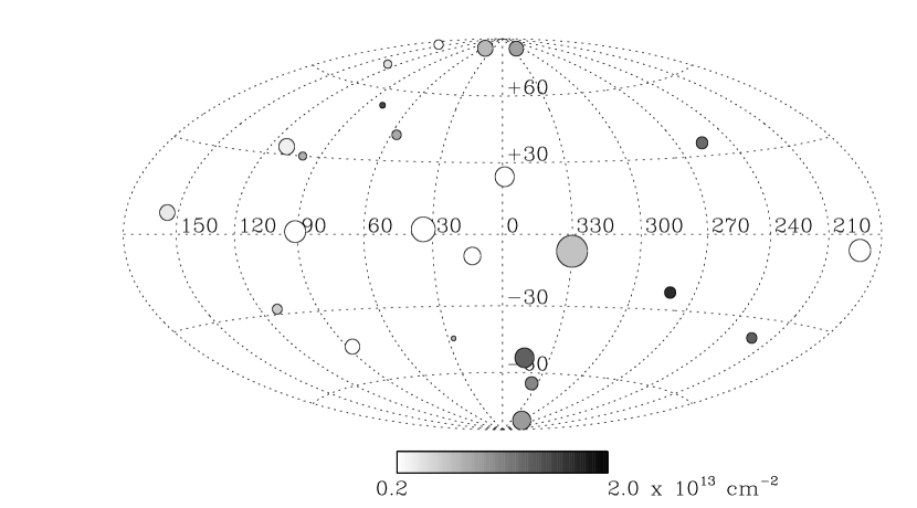
Figure 8: The distribution of O vi column density is plotted on an Aitoff projection of the sky. Each of the 25 stars in the survey are plotted as a shaded circle. The diameter of the circle is inversely proportional to the star’s distance, with a diameter of 5 degrees corresponding to a distance of 50 pc. The gray-scale shading is proportional to the O vi column density along that line of sight, with a scaling as shown in the color bar.

In Figure 8, we show the distribution of O vi absorption on the sky. In this plot, the size of the circle around each survey star is inversely proportional to its distance. Each circle has a gray-scale shading proportional to the column density along that line of sight, with darker shades representing higher column densities. The lines of sight with Galactic longitudes $210^{\circ}\lesssim l\lesssim 340^{\circ}$ and negative latitudes appear to have higher O vi column densities than elsewhere, although this trend is somewhat weakened by the likelihood that the O vi column densities towards WD 2211$-$495 and WD 2331$-$475, which are both at approximately Galactic coordinates ($l\sim 340^{\circ}$, $b\sim-60^{\circ}$), are contaminated by photospheric absorption (see §2.4).

Armed with column densities and distances, we can compute the space density of O vi, $\langle n($O vi$)\rangle$ (in cm^-3). There are several different methods that can be employed to do this. Jenkins (1978b) computed the value of $\Sigma N/\Sigma r$; the total column density of O vi for all lines of sight divided by the total effective path length to all stars (the effective path length is the equivalent distance of the star if it were in the Galactic plane, taking into account the decrease in density of O vi away from the plane). Using this definition, Jenkins (1978b) found an O vi density in the Galactic plane of $2.8\times 10^{-8}$ cm^-3, or $2.1\times 10^{-8}$ cm^-3 after discarding several lines of sight with “anomalous” column densities. Another method is just to compute the mean of all values of $N_{i}($O vi$)/r_{i}$. However, this method tends to overweight lines of sight with anomalous densities. This can be alleviated by using an inverse variance weighting,

$$\langle n(\mathrm{OVI})\rangle=s^{2}{\sum_{i}{N_{i}\over r_{i}}\sigma_{i}^{-2}}$$

where $s^{2}=1/{\sum_{i}\sigma^{-2}}$ is the variance of $\langle n($O vi$)\rangle$, $\sigma_{i}$ is the uncertainty in $(N_{i}/r_{i})$, $N_{i}$ is the column density of O vi and $r_{i}$ the effective distance, respectively, for the $i$th star. Using all 25 stars in the sample, we find an inverse variance weighted mean density of $1.9\pm 0.25\times 10^{-8}$ cm^-3, and an unweighted mean density is $2.45\times 10^{-8}$ cm^-3. The value computed from $\Sigma N/\Sigma r$ is approximately the same at $2.36\times 10^{-8}$ cm^-3, and is comparable to the value found by (Jenkins, 1978b) over much larger distances in the Galactic disk. A more recent determination of the Galactic disk O vi density has been made from a FUSE survey of 150 stars (Jenkins et al., 2001; Bowen et al., 2004). They find a median value of $N_{i}($O vi$)/r_{i}$ (measured for each sightline $i$) of $1.7\times 10^{-8}$ cm^-3. We find a median value of the O vi density from our LISM survey of $1.9\times 10^{-8}$ cm^-3. In summary, the space density of O vi that we observe locally is about the same, or somewhat larger than, the average for the Galactic disk over kpc scales.

Shelton & Cox (1994) reanalyzed the Copernicus data and included a contribution to the O vi column density from the Local Bubble along all lines of sight. Based on the Copernicus data alone, which had few stars at distances of less than 100 pc, they concluded that the LB contributed an O vi column density of $1.6\times 10^{13}$ cm^-2, and hence the mean space density in the Galactic plane outside the LB was lower than found by (Jenkins, 1978b). However, our survey indicates that the average O vi column density out to a distance of 100 pc from the Sun (the approximate distance to the edge of the LB in the Galactic plane) is $\sim 7\times 10^{12}$ cm^-2, based on our measured unweighted mean space density of $2.45\times 10^{-8}$ cm^-3.

We have performed some numerical simulations which show that our LISM survey is consistent with a scenario in which $\sim 6$ O vi producing clouds or interfaces per kpc are randomly distributed in space, each with a column density of $\sim 1.25\times 10^{13}$ cm^-2. This distribution of clouds predicts a dispersion in the O vi space densities that is consistent with that measured for the 25 lines of sight in the LISM survey. Hence, O vi absorption in the LISM appears to have a distribution quite similar to, or slightly larger than, much longer lines of sight in the Galactic disk. We find this to be a somewhat remarkable result, since we know that the Sun sits roughly in the middle of a supernova cavity – the LB. If hot bubbles only make up $\sim 20$% by volume of the Galactic disk, then the distance between bubbles should be fairly large. If O vi is formed in these hot regions of space, either at the interfaces with cool clouds or in condensation regions inside the bubbles, then the volume density of O vi producing regions in the disk should be lower than it is locally. Possibly the discrepancy is due to the quenching of conduction by magnetic fields on local cloud surfaces (i.e. without such quenching, the local space density of O vi would be higher), and/or that the conditions under which O vi is formed locally is not representative of the Galactic disk in general.

In the McKee & Ostriker (1977) theory of the ISM, cool clouds reside in a pervasive, hot ($T=10^{6}$ K) interstellar medium which is thermally stabilized by cloud evaporation. However, if conduction at cloud interfaces is largely quenched, then there will be little or no cloud evaporation. If magnetic shielding of conduction is common throughout the disk (as proposed here for the LISM), then the structure of the general ISM must be quite unlike that proposed by McKee & Ostriker (1977).

3.3 The Delayed Recombination Model

Breitschwerdt & Schmutzler (1994) have proposed a “delayed recombination” model for the Local Bubble in which an adiabatic expansion of hot gas is powered by supernovae. The gas cools quickly as it expands, and highly ionized stages are “frozen in” to the gas. The observed soft X-ray emission is then due to delayed recombination at low kinetic temperatures. In this model, the intercloud medium has a kinetic temperature of $\sim 50,000$ K and an electron density of $0.024$ cm^-3, yielding $P/k\sim 2600$ cm^-3 K. This ameliorates the pressure balance problem, which is a strong selling point of this model. Let us now consider the expected O vi production within the LB from this model. The column density of O vi along a path of length $l$ is $N($O vi$)\approx\xi($O vi$)\delta($O$)X($O$)n_{e}(n_{H}/n_{e})l$ cm^-2, where $\xi$(O vi) is the ionization fraction of O vi, $\delta$(O) is the linear depletion of oxygen onto dust grains, $X$(O) is the abundance of oxygen relative to hydrogen, and $n_{H}/n_{e}=0.83$ for a fully ionized gas that is 10% helium. Shapiro & Moore (1976) have computed models for the non-equilibrium radiative cooling of an optically thin gas which has been shock heated to $10^{6}$ K and allowed to cool to $10^{4}$ K, which is less extreme than the adiabatic cooling in the Breitschwerdt & Schmutzler (1994) model. Even after the gas has cooled to $T=5\times 10^{4}$ K, there is still significant fractions of O⁺⁵ and O⁺⁶ in the gas – in particular, $\xi$(O vi)$\sim 0.015$ (see Figure $5d$ in Shapiro & Moore (1976)). Adopting a solar abundance of oxygen of $X($O$)=4.57\times 10^{-4}$ (Asplund et al., 2004), a path length of 100 pc, and virtually no depletion ($\delta($O$)=1.0$) (Sofia & Meyer, 2001), we then arrive at an expected column density of O vi of $N($O vi$)\sim 4.2\times 10^{13}$ cm^-2. This column density is ruled out by the observations reported here.

3.4 Supernova Cavity Models

Cox & Smith (1974), Slavin & Cox (1992), Shelton (1999) and Smith & Cox (2001) have investigated the formation of O vi in the cavities carved out in the ISM by supernova explosions. In these models, the O vi resides in two distinct regions, the hot interior and the cooler periphery. Each has different characteristics and will be discussed separately. Here, we will concentrate on the recent computations by Smith & Cox (2001) of a multiple explosion scenario for the formation of the LB. Their models B and G, in which 3 explosions occur during a 2 million year period, give results that are in relatively good agreement with soft x-ray and O vi absorption line results.

In these models, after $\sim 6$ Myr, the interior of the 100 pc radius cavity is still highly ionized. Assuming a density of $n\sim 0.005$ cm^-3, $T=10^{6}$ K, an ionization fraction of O vi of $\xi$(O vi) $=0.006$ (Shapiro & Moore, 1976), a path length of 75 pc, and no depletion, we expect an O vi column density of $N$(O vi)$=2.6\times 10^{12}$ cm^-2. A column density of this level thermally broadening in a million degree gas is too difficult to detect with the signal-to-noise in the current dataset.

O vii is the dominant ion in the outer parts of the cavity, where the gas density is higher and recombination is more effective. O vi is abundant only near the edge of the cavity. Smith & Cox (2001) indicate that the model most appropriate for the LB is intermediate between their models B and G, for which they predict average column densities for O vi of 0.8 and $2.8\times 10^{13}$ cm^-2, respectively, for a line of sight from the center to edge of the bubble. This estimate is for the diffuse medium only, and does not include any contribution from interfaces of cool clouds embedded in the LB.

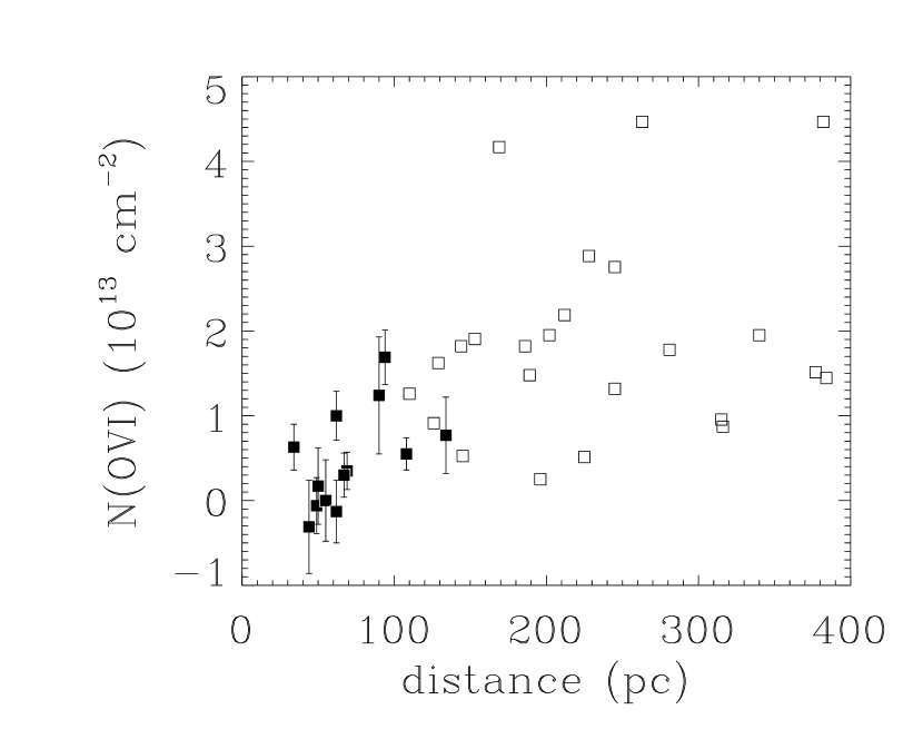
Figure 9: The column density of O vi versus stellar distance for stars at Galactic latitudes $|b|<35^{\circ}$. The solid squares are the data for the FUSE LISM targets reported in this paper. The open squares are column densities from Copernicus data, for stars at distances of $100-400$ pc (Jenkins, 1978a).

Let us restrict our attention to the stars in our LISM survey for which the Galactic latitude, $|b|<35^{\circ}$, so that the star’s distance is more closely related to the distance to the bubble wall (e.g. it can be seen from Figure 2 that the LB has a “chimney” appearance, so that stars at high Galactic latitude are far from the wall of the local cavity). Thirteen stars in our survey satisfy this constraint on Galactic latitude. In Figure 9, we have plotted O vi column density versus distance of the star from the Sun for these 13 stars, plus the data for stars at distances of $100-400$ pc with $|b|<35^{\circ}$ from the earlier Copernicus study by Jenkins (1978a). There does not appear to be any convincing evidence for a sharp rise in O vi column density at a distance corresponding to the edge of the cavity from this plot. In Figures 1 and 2 we also show the location of the stars in the LISM survey relative to the cavity wall (as defined by Sfeir et al. (1999)), and we find that there is no correlation between the strength of O vi absorption and closeness to the wall. These conclusions, however, are based on a relatively small sample of lines of sight. Finally, we also point out that the O vi column density intermediate between models B and G (Smith & Cox, 2001) of $\sim 2\times 10^{13}$ cm^-2 is substantially larger than the observed mean column density of $\sim 7\times 10^{12}$ cm^-2 within the LB (assuming a path length of 100 pc). The eight stars in our survey having large H i column densities, logN(H i)$>19.0$, implying that they are near the wall of the cavity, have an average O vi column density of $5.8\times 10^{12}$ cm^-2, which is also substantially less than the column density predicted by models B and G.

4 Conclusions

We have carried out a survey of interstellar O vi absorption along the lines of sight to 25 white dwarfs in the LISM, after excluding 4 stars that display strong photospheric O vi. O vi absorption is weak or absent in most lines of sight, and has a somewhat “patchy” distribution (a scatter that is much larger than the measurement uncertainties). The O vi absorption in several stars may be due in part to photospheric or circumstellar absorption, which would imply even smaller column densities in the ISM for these lines of sight. We find a mean line width, based on computing mean absolute deviations for the O vi line profiles, of $16\pm 2$ km s^-1, corresponding to a standard deviation of 20 km s^-1. This line width is about 30% larger than expected for a single component absorption line formed at 300,000 K and convolved with the FUSE instrumental resolution.

The general picture that emerges from these observations is one in which the observed O vi absorption is produced over limited regions on the surfaces of clouds within the Local Bubble. Conduction must be quenched over much of the surface area of each cloud, presumably by magnetic fields. Indeed, we know that the Sun is located within a cool cloud inside the hot LB, and all lines of sight should penetrate at least one cloud interface, if not several. Quite sophisticated theoretical models on the other hand indicate that an unshielded interface should produce an O vi column density of $\sim 10^{13}$ cm^-3, yet many of our lines of sight indicate columns significantly below this value. The mean O vi space density in our LISM survey is $\sim 2.4\times 10^{-8}$ cm^-3, and is comparable to, or slightly larger than, the value over much larger path lengths (400-1000 pc) in the Galactic plane determined by the Copernicus survey (Jenkins, 1978b). Out to a distance of $\sim 100$ pc from the Sun, corresponding roughly to the size of the Local Bubble in the Galactic plane, the average column density of O vi is $\sim 7\times 10^{12}$ cm^-2, or about half that estimated earlier (Shelton & Cox, 1994).

This picture, however, implies that there should be little EUV radiation from the evaporative interface between the LIC and the presumably hot interior of the Local Bubble, at odds with the models of Slavin & Frisch (2002), which have successfully explained a number of observations of the ionization in the LISM.

Table 1: Survey Star Data

WD Number	Alt. Name	Distance	logN(H i)	$l$	$b$	Type	Teff	Datasets
		pc	cm-2	deg	deg		(K)
0004$+$330	GD 2	108	19.80	111	$-28$	DA1	49,360	P2041101
0050$-$332	GD 659	58	18.40	299	$-84$	DA1.5	36,000	P2042001
0131$-$163	GD 984	104	…	167	$-75$	DA1+dM?	48,700	P2041201
0455$-$282	RE J0457$-$281	102	18.06	222	$-37$	DA1	57,200	P1041101
								P1041102
								P1041103
0501$+$527	G191$-$B2B	69	18.30	156	$+7$	DA1	56,000	S3070101
								P1041201
								P1041202
0501$-$289	RE J0503$-$289	90	…	230	$-35$	DO	70,000	P2041601
0549$+$158	GD 71	49	17.92	192	$-5$	DA1.5	32,750	P2041701
0715$-$704	…	94	19.32	282	$-23$	DA	43,600	P2042101
1017$-$138	…	90	18.68	256	$+35$	DA	32,000	P2041501
1211$+$332	HZ 21	115	…	175	$+80$	DO2	53,000	P2040801
								P2040802
1234$+$481	HS1234$+$481	129	19.13	130	$+69$	DA1	56,400	P2040901
1254$+$223	GD 153	73	17.92	317	$+84$	DA1.5	38,686	M1010401
								M1010402
								M1010403
								P2041801
1314$+$293	HZ 43	68	17.94	54	$+84$	DA1	50,560	P1042301
1529$+$486	RE J1529$+$483	184	18.30	79	$+53$	DA1	47,600	P2040101
1615$-$154	EG 118	55	…	359	$+24$	DA1.5	29,732	P2041901
1631$+$781	RE J1629$+$780	67	19.30	111	$+33$	DA1+dMe	44,560	P1042901
								P1042902
1634$-$573	HD149499B	34	18.80	330	$-7$	DO+KOV	49,500	M1031103
								M1031105
								S5140201
1636$+$351	KUV 16366$+$3506	113	19.57	57	$+41$	DA	37,200	P2040201
1800$+$685	KUV 1800$+$685	134	18.86	99	$+30$	DA1	46,000	P2041001
1845$+$019	Lanning 18	44	18.45	34	$+2$	DA1.5	30,000	P2040301
1847$-$223	…	62	19.55	13	$-9$	DA	31,600	P2040501
2004$-$605	RE J2009$-$602	62	19.32	337	$-33$	DA1	44,200	P2042201
2013$+$400	RE J2013$+$400	143	…	78	$+3$	DAO+dM	53,600	P2040401
2111$+$498	GD 394	50	18.60	91	$+1$	DA1.5	37,360	M1010704
								M1010706
								P1043601
2127$-$222	…	224	18.43	27	$-44$	DA	49,800	P2040601
2156$-$546	RE J2156$-$543	109	…	340	$-48$	DA	45,800	P2042301
2211$-$495	RE J2214$-$491	55	18.30	346	$-53$	DA1	63,500	M1030305
								P1043801
2309$+$105	GD 246	72	19.12	87	$-45$	DA1	58,700	P2042401
2331$-$475	RE J2334$-$471	82	17.90	335	$-65$	DA1	55,800	P1044201

Table 2: O vi $\lambda$1032 Measurements

WD Number	Wλ	N(O vi)	${\bar{v}}$	$v_{mad}$	Notes
	(mÅ)	($10^{13}$ cm-2)	(km s-1)	(km s-1)
0004$+$330	$6.9\pm 2.4$	$0.55\pm 0.19$	$+7$	…
0050$-$332	$11.3\pm 4.1$	$0.90\pm 0.33$	$+20$	$18$
0455$-$282	$16.6\pm 3.7$	$1.33\pm 0.30$	$-35$	$18$	1
0501$+$527	$4.4\pm 2.8$	$0.35\pm 0.22$	$+5$	…	2
0549$+$158	$-0.7\pm 4.1$	$-0.06\pm 0.33$	…	…
0715$-$704	$21.1\pm 4.0$	$1.69\pm 0.32$	$-4$	$20$
1017$-$138	$15.5\pm 8.6$	$1.24\pm 0.69$	…	…
1211$+$332	$-0.4\pm 3.7$	$-0.03\pm 0.30$	…	…
1234$+$481	$5.3\pm 8.3$	$0.43\pm 0.66$	…	…
1254$+$223	$10.7\pm 4.2$	$0.86\pm 0.33$	$+31$	$16$
1314$+$293	$8.7\pm 1.9$	$0.70\pm 0.15$	$+20$	$15$
1529$+$486	$18.8\pm 3.5$	$1.50\pm 0.28$	$+4$	$17$
1615$-$154	$-0.1\pm 6.0$	$0.00\pm 0.48$	…	…
1631$+$781	$3.7\pm 3.3$	$0.30\pm 0.26$	…	…
1634$-$573	$7.8\pm 3.4$	$0.63\pm 0.27$	$0$	$13$
1636$+$351	$10.1\pm 4.6$	$0.81\pm 0.37$	$+19$	…
1800$+$685	$9.6\pm 5.7$	$0.77\pm 0.45$	$+12$	…
1845$+$019	$-3.9\pm 6.8$	$-0.31\pm 0.55$	…	…
1847$-$223	$-1.7\pm 4.6$	$-0.13\pm 0.37$	…	…
2004$-$605	$12.5\pm 3.6$	$1.00\pm 0.29$	$+2$	$17$
2111$+$498	$2.1\pm 5.6$	$0.17\pm 0.45$	…	…
2127$-$222	$9.6\pm 4.4$	$0.77\pm 0.35$	$0$	…
2211$-$495	$16.4\pm 3.7$	$1.32\pm 0.29$	$+25$	$16$	2
2309$+$105	$0.4\pm 2.8$	$0.03\pm 0.23$	…	…
2331$-$475	$13.1\pm 3.7$	$1.05\pm 0.30$	$+19$	$15$	2

Note. — Equivalent widths were measured in the velocity interval $\pm 40$ km s^-1 centered on the expected position of O vi $\lambda$1036 relative to the C ii $\lambda$1036 line. (1) Significant absorption occurs outside the velocity integration limits for WD 0455$-$282. (2) The O vi line measurement is likely contaminated by photospheric absorption; see §2.4 for discussion.

Figure 1: Positions of the 13 white dwarfs from Table 1 with $|b|<35^{\circ}$, projected onto the Galactic Plane (solid squares). Overlayed on the plot (thin solid line) is the boundary of the Local Cavity as defined by 20 mÅ Na D absorption line equivalent widths from Lallement et al. (2003). The thick solid line is the boundary of the hot Local Bubble, as defined by the 0.25 keV soft x-ray emission (regions affected by contaminating sources are represented by dashed lines) (Snowden et al., 1998). The distance to the boundary of the LB is a matter of some debate (see text), and may coincide with the Local Cavity. The Galactic center is in the direction of the positive X axis, and Galactic longitude, $l=90^{\circ}$, is in the positive Y axis direction.

Figure 2: Same as Figure 1, except this is a projection onto the Meridional plane, for all 25 white dwarfs listed in Table 1. The Galactic center is in the direction of the positive X axis, and Galactic latitude, $b=90^{\circ}$, is in the positive Y axis direction.

Figure 3: Spectrum of WD 2156$-$546 taken through the MDRS aperture in the LiF1A channel, showing strong photospheric absorption in both members of the O vi doublet at $\lambda$1031.93 and $\lambda$1037.62. Also present in the spectrum are interstellar lines of C ii $\lambda$1036.34 and O i $\lambda$1039.23.

Figure 4: Normalized spectra of the 25 white dwarfs from Table 2 are plotted, centered on the O vi $\lambda$1031.926 line as a function of velocity. The velocity zero point is set relative to the centroid of the C ii $\lambda$1036.336 line.

Figure 5: Equivalent width of the O vi $\lambda$1031.9 photospheric line vs. T_eff for a grid of oxygen abundances, log(O/H), based on NLTE white dwarf model atmospheres with $\log g=8$.

Figure 6: Plots of 5 white dwarf spectra containing metals in their atmospheres. The data, shown as a histogram plot, is the same as that in Figure 4, but the wavelength zero-point has been shifted to put the stellar lines at their laboratory wavelengths. The solid dark curve overlayed is a photospheric model. The strongest stellar lines visible here are P iv $\lambda$1030.51, O vi $\lambda$1031.93, and P iv $\lambda$1033.11. A host of Fe iii photospheric lines are present in the spectrum of WD 2111$+$498, most notably the lines at 1030.92, 1032.12, and 1033.30 Å.

Figure 7: The column density of O vi versus H i.

References

- Andersson et al. (2002) Andersson, B-G., Idzi, R. Uomoto, A., Wannier, P., Chen, B. & Jorgensen, A. 2002, AJ, 124, 2164
- Asplund et al. (2004) Asplund, M., Grevesse, N., Sauval, A. J., Prieto, C. A. & Kiselman, D. 2004, A&A, 417, 751
- Avillez (2000) Avillez, M. A. 2000, MNRAS, 315, 479
- Avillez & Breitschwerdt (2004) Avillez, M. A. & Breitschwerdt, D. 2004, Ap&SS, 289, 479
- Barstow et al. (2001) Barstow, M. et al. 2001, in 12th European Conf. on White Dwarfs, ASP Conf. Proc., Vol. 226, ed. J. L. Provencal, H. L. Shipman, J. McDonald & S. Goodchild, San Francisco: Astron. Soc. of the Pacific, 94
- Barstow et al. (2002) Barstow, M. et al. 2002, MNRAS, 330, 425
- Barstow et al. (2003) Barstow, M.A., Good, S.A., Holberg, J.B., Hubeny, I., Bannister, N.P., Bruhweiler, F.C., Burleigh, M.R., & Napiwotzki, R. 2003, MNRAS, 341, 870
- Berghöfer & Breitschwerdt (2002) Berghöfer, T. & Breitschwerdt, D. 2002, A&A, 390, 299
- Borkowski et al. (1990) Borkowski, K., Balbus, S. & Fristrom, C. 1990, ApJ, 355, 501
- Bowen et al. (2004) Bowen, D., Jenkins, E., Tripp, T., Sembach, K., & Savage, B. 2004, in Astrophysics in the Far Ultraviolet, ASP Conf Series, ed. Sonneborn, G., Moos, H., & Andersson, B-G, in press (astro-ph/0410008)
- Bowyer, Field & Mack (1968) Bowyer, S., Field, G. & Mack, J. 1968, Nature, 217, 32