Particle Acceleration at shocks: some modern aspects of an old problem

Abstract

The acceleration of charged particles at astrophysical collisionless shock waves is one of the best studied processes for the energization of particles to ultrarelativistic energies, required by multifrequency observations in a variety of astrophysical situations. In this paper we discuss some work aimed at describing one of the main progresses made in the theory of shock acceleration, namely the introduction of the non-linear backreaction of the accelerated particles onto the shocked fluid. The implications for the investigation of the origin of ultra high energy cosmic rays will be discussed.

1 Introduction

Suprathermal charged particles scattering back and forth across the surface of a shock wave gain energy. The concept of stochastic energization due to randomly moving inhomogeneities was first proposed by Fermi [1]. In that original version, the acceleration process is easily shown to be efficient only at the second order in the parameter $V$, the average speed of the irregularities in the structure of the magnetic field, in units of the speed of light. For non-relativistic motion, $V\ll 1$, the mechanism is not very attractive. The generalization of this idea to the case of a shock wave was first proposed in [2, 3, 4, 5] and is nicely summarized in several recent reviews [6, 7, 8, 9, 10], where the efficiency of the process was found to be now at the first order in $V$. Since these pioneering papers the process of particle acceleration at shock waves has been investigated in many aspects and is now believed to be at work in a variety of astrophysical environments. In fact we do observe shocks everywhere, from the solar system to the interplanetary medium, from the supernovae environments to the formation of the large scale structure of the universe. All these are therefore sites of both heating of the medium crossing the shock surface and generation of suprathermal particles. The two phenomena are most likely different aspects of the same process, also responsible for the formation of the collisionless shock itself. One of the major developments in the theory of particle acceleration at astrophysical shock waves has consisted of removing the assumption of test particle, namely the assumption that the accelerated particles could not affect the dynamics of the shocked fluid . Two approaches have been proposed to treat this intrinsically non-linear problem: the two fluid models [11, 12, 13, 14, 15] and the kinetic models [16, 17, 18, 19], while numerous attempts to simulate numerically the process of particle acceleration have also been made [9, 20, 21, 22, 23, 24, 25]. The two fluid models treat the accelerated particles as a separate fluid, contributing a pressure and energy density which enter the usual conservation laws at the shock surface. By construction, these models do not provide information about the spectrum of the accelerated particles, while correctly describing the detailed dynamics of the fluids involved. The kinetic models on the other hand have a potential predictive power in terms of both dynamics and spectral shape of the accelerated particles.

All these considerations hold in principle for all shocks but in practice most of the work has been done for the case of newtonian shock waves (however see [26] for an extension to relativistic shocks). Astrophysical studies have shown that there are plenty of examples in Nature of fluids moving at relativistic speeds, and generating shock waves. The generalization of the process of particle acceleration to the relativistic case represents in our opinion the second major development of the theory (Baring, these proceedings).

In this paper, we will not present a review of all the current efforts in the investigation of shock acceleration. We will rather concentrate our attention upon some recent work in the direction of accounting for the non-linear backreaction of the accelerated particles.

2 The non-linear backreaction: breaking the test particle approximation

The original theory of particle acceleration was based on the assumption that the accelerated particles represent a passive fluid, with no dynamical backreaction on the background plasmas involved. Within the context of this approximation, several independent approaches [4, 6] give the spectrum of the accelerated particles in the form of a power law in momentum $f(p)=f_{0}(p/p_{0})^{-\alpha}$, where the slope $\alpha$ is related in a unique way to the Mach number $M$ of the upstream fluid as seen in the shock frame, through the expression $\alpha=4M^{2}/(M^{2}-1)$ (here we asumed that the adiabatic index of the background gas is $\gamma_{g}=5/3$). This result is easily shown by using the diffusion-convection equation in one dimension for a stationary situation (namely $\partial f/\partial t=0$):

$$\frac{\partial}{\partial x}\left[D\frac{\partial}{\partial x}f(x,p)\right]-u\frac{\partial f(x,p)}{\partial x}+$$

$$+\frac{1}{3}\frac{du}{dx}~{}p~{}\frac{\partial f(x,p)}{\partial p}+Q(x,p)=0,$$ (1)

where $D$ is the diffusion coefficient, $f(x,p)$ is the distribution function of accelerated particles in phase space and $Q$ is the injection function, which we will assume to be a Dirac delta function at the shock surface $x=0$ in the downstream fluid ($x=0^{+}$). The function $f$ is normalized in such a way that the total number of accelerated particles is given by $\int_{p_{inj}}^{p_{max}}dp4\pi p^{2}f(p)$.

As a first step, we integrate eq. 1 around $x=0$, from $x=0^{-}$ to $x=0^{+}$, which we denote as points “1” and “2” respectively, so that we get

$$\left[D\frac{\partial f}{\partial x}\right]_{2}-\left[D\frac{\partial f}{\partial x}\right]_{1}+\frac{1}{3}p\frac{df_{0}}{dp}(u_{2}-u_{1})+Q_{0}(p)=0,$$ (2)

where $u_{1}$ ($u_{2}$) is the fluid speed immediately upstream (downstream) of the shock and $f_{0}$ is the particle distribution function at the shock location. By requiring that the distribution function downstream is independent of the spatial coordinate (homogeneity), we obtain $\left[D\frac{\partial f}{\partial x}\right]_{2}=0$, so that the boundary condition at the shock can be rewritten as

$$\left[D\frac{\partial f}{\partial x}\right]_{1}=\frac{1}{3}p\frac{df_{0}}{dp}(u_{2}-u_{1})+Q_{0}(p).$$ (3)

We can now perform the integration of eq. (1) from $x=-\infty$ to $x=0^{-}$ (point “1”), in order to take into account the boundary condition at upstream infinity. Using eq. (3) we obtain

$$\frac{1}{3}p\frac{df_{0}}{dp}(u_{2}-u_{1})-u_{1}f_{0}+Q_{0}(p)=0.$$ (4)

The solution of this equation for $f_{0}$ has the form of a power law $f_{0}\propto p^{-\alpha}$ with slope $\alpha=3u_{1}/(u_{1}-u_{2})=3r/(r-1)$, where we introduced the compression factor $r=u_{1}/u_{2}$ at the shock. For a strong shock $r\to 4$ and we find the well known asymptotic spectrum $f_{0}\to p^{-4}$, or $N(E)\propto E^{-2}$ in terms of energy (here again we assumed that the adiabatic index of the background gas is $\gamma_{g}=5/3$.

Why should we expect this simple result to be affected by the assumption of test particles? There are three physical arguments that may serve as plausibility arguments to investigate the effects of possible backreactions: 1) the spectrum $E^{-2}$ is logarithmically divergent in its energy content, so that even choosing a maximum momentum, it is possible that the energy density in the form of accelerated particles becomes comparable with the kinetic pressure, making the assumption of test particles untenable; 2) if the non thermal pressure becomes appreciable, the effective adiabatic index can get closer to $4/3$ rather than $5/3$, making the shock more compressive and the spectrum of accelerated particles even more divergent; 3) more divergent spectra imply larger fluxes of escaping particles at the maximum momentum, which make the shock radiative-like, again implying a larger compression and flatter spectra.

All the three issues raised here point toward the direction of making the backreaction more severe rather than alleviating its effect, therefore a run-away reaction seems likely, which drives the shock toward a strongly non-linear cosmic ray modified configuration (here the term cosmic rays is used in a general way to indicate the accelerated particles).

We can describe the expected effects on the basis of the following simple argument: if, as is usually the case, the diffusion coefficient increases with the momentum of the particles, we can expect that particles with larger momenta will diffuse farther from the shock surface in the upstream section of the gas. At large distances from the shock, only the high energy particles will be present, while lower energy particles will populate the regions closer to the shock surface. There is some critical distance which corresponds to the typical diffusion length of the particles with the maximum momentum achievable, $p_{max}$. At this distance, the pressure of the cosmic rays is basically zero and the fluid is unperturbed. On the other hand, moving inward, toward the shock, an increasing number of accelerated particles is present, and their pressure contributes to the local pressure budget by slowing down the fluid (in the shock frame). This effect causes the fluid speed upstream to be space-dependent, and decreasing while approaching the shock surface. The region of slow decrease of the fluid velocity is usually called the precursor. The shock, which may now be substantially weakened by the effect of the accelerated particles, is usually called subshock.

It is useful to introduce the two quantities $R_{sub}=u_{1}/u_{2}$ and $R_{tot}=u_{0}/u_{2}$, which are respectively the compression factor at the gas subshock and the total compression factor between upstream infinity and downstream. Here $u_{0}$, $u_{1}$ and $u_{2}$ are the fluid speeds at upstream infinity, upstream of the subshock and downstream respectively. The two compression factors would be equal in the test particle approximation. For a modified shock, $R_{tot}$ can attain values much larger than $R_{sub}$ and more in general, much larger than $4$, which is the maximum value achievable for an ordinary strong non-relativistic shock.

The shape of the particle spectrum is still determined by some jump in the velocity field, but this quantity is now local: at low energies, the compression felt by the particles is $\sim R_{sub}$, while at $p\sim p_{max}$ the effective compression is $\sim R_{tot}$. It follows that, since $R_{sub}<R_{tot}$, the spectrum at low energies is steeper than that at higher energies: the overall spectrum at cosmic ray modified shocks is therefore expected to have a concave shape.

In the following we will describe the effects of the particle backreaction following the kinetic semi-analytical approach proposed in [18, 19], and we will use the most general formalism, which includes the possible presence of seed pre-accelerated particles in the environment in which the shock propagates. We repeat here the steps illustrated above for the linear case. Integrating again eq. 1 around $x=0$, from $x=0^{-}$ to $x=0^{+}$, we get Eq. 3, after invoking the homogeneity of the particle distribution downstream.

Performing now the integration of eq. 1 from $x=-\infty$ to $x=0^{-}$ we obtain

$$\frac{1}{3}p\frac{df_{0}}{dp}(u_{2}-u_{1})-u_{1}f_{0}+u_{0}f_{\infty}+Q_{0}(p)+$$

$$\int_{-\infty}^{0^{-}}dxf\frac{du}{dx}+\frac{1}{3}\int_{-\infty}^{0^{-}}dx\frac{du}{dx}p\frac{\partial f}{\partial p}=0.$$ (5)

Here $f_{\infty}$ represents the distribution of seed pre-accelerated particles possibly present at upstream infinity.

We can now introduce the quantity $u_{p}$ defined as

$$u_{p}=u_{1}-\frac{1}{f_{0}}\int_{-\infty}^{0^{-}}dx\frac{du}{dx}f(x,p),$$ (6)

whose physical meaning is instrumental to understand the nonlinear backreaction of the accelerated particles. The function $u_{p}$ is the average fluid velocity experienced by particles with momentum $p$ while diffusing upstream away from the shock surface. In other words, the effect of the average is that, instead of a constant speed $u_{1}$ upstream, a particle with momentum $p$ experiences a spatially variable speed, due to the pressure of the accelerated particles that is slowing down the fluid. Since the diffusion coefficient is in general $p$-dependent, particles with different energies feel a different compression coefficient, higher at higher energies if, as expected, the diffusion coefficient is an increasing function of momentum.

With the introduction of $u_{p}$, eq. (5) becomes

$$\frac{1}{3}p\frac{df_{0}}{dp}(u_{2}-u_{p})-f_{0}\left[u_{p}+\frac{1}{3}p\frac{du_{p}}{dp}\right]+u_{0}f_{\infty}+Q_{0}(p)=0,$$ (7)

The solution of this equation can be written in the following implicit form:

$$f_{0}(p)=f_{0}^{reacc}(p)+f_{0}^{inj}(p)=$$

$$\int_{p_{0}}^{p}\frac{d{\bar{p}}}{{\bar{p}}}\frac{3\left[u_{0}f_{\infty}({\bar{p}})+Q_{0}({\bar{p}})\right]}{u_{\bar{p}}-u_{2}}\times$$

$$\exp\left\{-\int_{\bar{p}}^{p}\frac{dp^{\prime}}{p^{\prime}}\frac{3}{u_{p^{\prime}}-u_{2}}\left[u_{p^{\prime}}+\frac{1}{3}p^{\prime}\frac{du_{p^{\prime}}}{dp^{\prime}}\right]\right\}.$$ (8)

In the case of monochromatic injection with momentum $p_{inj}$ at the shock surface, we can write

$$Q_{0}(p)=\frac{\eta n_{gas,1}u_{1}}{4\pi p_{inj}^{2}}\delta(p-p_{inj}),$$ (9)

where $n_{gas,1}$ is the gas density immediately upstream ($x=0^{-}$) and $\eta$ parametrizes the fraction of the particles crossing the shock which are going to take part in the acceleration process.

In terms of $R_{sub}$ and $R_{tot}$, introduced above, the density immediately upstream is $n_{gas,1}=(\rho_{0}/m_{p})R_{tot}/R_{sub}$. We can introduce the dimensionless quantity $U(p)=u_{p}/u_{0}$ so that

$$f_{0}(p)=\frac{3R_{tot}}{R_{tot}U(p)-1}\int_{p_{0}}^{p}\frac{d{\bar{p}}}{{\bar{p}}}f_{\infty}({\bar{p}})\times$$

$$\exp\left\{-\int_{\bar{p}}^{p}\frac{dp^{\prime}}{p^{\prime}}\frac{3R_{tot}U(p^{\prime})}{R_{tot}U(p^{\prime})-1}\right\}+$$

$$\left(\frac{3R_{sub}}{R_{tot}U(p)-1}\right)\frac{\eta n_{gas,1}}{4\pi p_{inj}^{3}}\times$$

$$\exp\left\{-\int_{p_{inj}}^{p}\frac{dp^{\prime}}{p^{\prime}}\frac{3R_{tot}U(p^{\prime})}{R_{tot}U(p^{\prime})-1}\right\}.$$ (10)

The structure of the fluid upstream of the shock and the corresponding spectrum of accelerated particles is determined if the velocity field $U(p)=u_{p}/u_{0}$ is known. The nonlinearity of the problem reflects in the fact that $U(p)$ is in turn a function of $f_{0}$ as it is clear from the definition of $u_{p}$. In order to solve the problem we need to write the equations for the thermodynamics of the system including the gas, the reaccelerated cosmic rays, the cosmic rays accelerated from the thermal pool and the shock itself.

The velocity, density and thermodynamic properties of the fluid can be determined by the mass and momentum conservation equations, with the inclusion of the pressure of the accelerated particles and of the preexisting cosmic rays. We write these equations between a point far upstream ($x=-\infty$), where the fluid velocity is $u_{0}$ and the density is $\rho_{0}=mn_{gas,0}$, and the point where the fluid upstream velocity is $u_{p}$ (density $\rho_{p}$). The index $p$ denotes quantities measured at the point where the fluid velocity is $u_{p}$, namely at the point $x_{p}$ that can be reached only by particles with momentum $\geq p$.

The mass conservation implies:

$$\rho_{0}u_{0}=\rho_{p}u_{p}.$$ (11)

Conservation of momentum reads:

$$\rho_{0}u_{0}^{2}+P_{g,0}+P_{CR,0}=\rho_{p}u_{p}^{2}+P_{g,p}+P_{CR,p},$$ (12)

where $P_{g,0}$ and $P_{g,p}$ are the gas pressures at the points $x=-\infty$ and $x=x_{p}$ respectively, and $P_{CR,p}$ is the pressure in accelerated particles at the point $x_{p}$ (we used the symbol $CR$ to mean cosmic rays, in the sense of accelerated particles). The mass flow in the form of accelerated particles has reasonably been neglected.

Our basic assumption, similar to that used in [27], is that the diffusion is $p$-dependent and more specifically that the diffusion coefficient $D(p)$ is an increasing function of $p$. Therefore the typical distance that a particle with momentum $p$ moves away from the shock is approximately $\Delta x\sim D(p)/u_{p}$, larger for high energy particles than for lower energy particles. As a consequence, at each given point $x_{p}$ only particles with momentum larger than $p$ are able to affect appreciably the fluid. Strictly speaking the validity of the assumption depends on how strongly the diffusion coefficient depends on the momentum $p$.

The cosmic ray pressure at $x_{p}$ is the sum of two terms: one is the pressure contributed by the adiabatic compression of the cosmic rays at upstream infinity, and the second is the pressure of the particles accelerated or reaccelerated at the shock (${\tilde{P}}_{CR}(p)$) and able to reach the position $x_{p}$. Since only particles with momentum larger than $p$ can reach the point $x=x_{p}$, we can write

$$P_{CR,p}=P_{CR,0}\left(\frac{u_{0}}{u_{p}}\right)^{\gamma_{CR}}+{\tilde{P}}_{CR}(p)\simeq$$

$$\simeq P_{CR,0}(p)\left(\frac{u_{0}}{u_{p}}\right)^{\gamma_{CR}}+\frac{4\pi}{3}\int_{p}^{p_{max}}dpp^{3}v(p)f_{0}(p),$$ (13)

where $v(p)$ is the velocity of particles with momentum $p$, $p_{max}$ is the maximum momentum achievable in the specific situation under investigation, and $\gamma_{CR}$ is the adiabatic index for the accelerated particles. In Eq. 13 the first term represents the adiabatic compression of the pressure of the seed particles advected from upstream infinity, while the second term represents the pressure in the freshly accelerated particles at the position $x_{p}$.

In the following we use $\gamma_{CR}=4/3$ (see [19] for a detailed discussion of the reasons for this choice).

The pressure of cosmic rays at upstream infinity is simply

$$P_{CR,0}=\frac{4\pi}{3}\int_{p_{min}}^{p_{max}}dpp^{3}v(p)f_{\infty}(p),$$ (14)

where $p_{min}$ is some minimum momentum in the spectrum of seed particles.

From eq. (12) we can see that there is a maximum distance, corresponding to the propagation of particles with momentum $p_{max}$ such that at larger distances the fluid is unaffected by the accelerated particles and $u_{p}=u_{0}$.

We will show later that for strongly modified shocks the integral in eq. (13) is dominated by the region $p\sim p_{max}$. This improves even more the validity of our approximation $P_{CR,p}=P_{CR}(>p)$. This also suggests that different choices for the diffusion coefficient $D(p)$ may affect the value of $p_{max}$, but at fixed $p_{max}$ the spectra of the accelerated particles should not change in a significant way.

Assuming an adiabatic compression of the gas in the upstream region, we can write

$$P_{g,p}=P_{g,0}\left(\frac{\rho_{p}}{\rho_{0}}\right)^{\gamma_{g}}=P_{g,0}\left(\frac{u_{0}}{u_{p}}\right)^{\gamma_{g}},$$ (15)

where we used mass conservation, eq. (11). The gas pressure far upstream is $P_{g,0}=\rho_{0}u_{0}^{2}/(\gamma_{g}M_{0}^{2})$, where $\gamma_{g}$ is the ratio of specific heats for the gas ($\gamma_{g}=5/3$ for an ideal gas) and $M_{0}$ is the Mach number of the fluid far upstream.

We introduce now a parameter $\xi_{CR}$ that quantifies the relative weight of the cosmic ray pressure at upstream infinity compared with the pressure of the gas at the same location, $\xi_{CR}=P_{CR,0}/P_{g,0}$. Using this parameter and the definition of the function $U(p)$, the equation for momentum conservation becomes

$$\frac{dU}{dp}\left[1-\frac{\gamma_{CR}}{\gamma_{g}}\frac{\xi_{CR}}{M_{0}^{2}}U^{-(\gamma_{CR}+1)}-\frac{1}{M_{0}^{2}}U^{-(\gamma_{g}+1)}\right]+$$

$$\frac{1}{\rho_{0}u_{0}^{2}}\frac{d{\tilde{P}}_{CR}}{dp}=0.$$ (16)

Using the definition of ${\tilde{P}}_{CR}$ and multiplying by $p$, this equation becomes

$$p\frac{dU}{dp}\left[1-\frac{\gamma_{CR}}{\gamma_{g}}\frac{\xi_{CR}}{M_{0}^{2}}U^{-(\gamma_{CR}+1)}-\frac{1}{M_{0}^{2}}U^{-(\gamma_{g}+1)}\right]=$$

$$\frac{4\pi}{3\rho_{0}u_{0}^{2}}p^{4}v(p)f_{0}(p),$$ (17)

where $f_{0}$ depends on $U(p)$ as written in eq. (10). Eq. (17) is therefore an integral-differential nonlinear equation for $U(p)$. The solution of this equation also provides the spectrum of the accelerated particles.

The last missing piece is the connection between $R_{sub}$ and $R_{tot}$, the two compression factors appearing in eq. (8). The compression factor at the gas shock around $x=0$ can be written in terms of the Mach number $M_{1}$ of the gas immediately upstream through the well known expression

$$R_{sub}=\frac{(\gamma_{g}+1)M_{1}^{2}}{(\gamma_{g}-1)M_{1}^{2}+2}.$$ (18)

On the other hand, if the upstream gas evolution is adiabatic, then the Mach number at $x=0^{-}$ can be written in terms of the Mach number of the fluid at upstream infinity $M_{0}$ as

$$M_{1}^{2}=M_{0}^{2}\left(\frac{u_{1}}{u_{0}}\right)^{\gamma_{g}+1}=M_{0}^{2}\left(\frac{R_{sub}}{R_{tot}}\right)^{\gamma_{g}+1},$$

so that from the expression for $R_{sub}$ we obtain

$$R_{tot}=M_{0}^{\frac{2}{\gamma_{g}+1}}\left[\frac{(\gamma_{g}+1)R_{sub}^{\gamma_{g}}-(\gamma_{g}-1)R_{sub}^{\gamma_{g}+1}}{2}\right]^{\frac{1}{\gamma_{g}+1}}.$$ (19)

Now that an expression between $R_{sub}$ and $R_{tot}$ has been found, eq. (17) basically is an equation for $R_{sub}$, with the boundary condition that $U(p_{max})=1$. Finding the value of $R_{sub}$ (and the corresponding value for $R_{tot}$) such that $U(p_{max})=1$ also provides the whole function $U(p)$ and, through eq. (8), the distribution function $f_{0}(p)$ for the particles resulting from acceleration and reacceleration in the nonlinear regime. When the backreaction of the accelerated particles is small, the test particle solution is recovered.

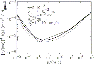
Figure 1: Example of concave non-linear spectrum obtained with the calculation of [18, 19] and described here. The parameters used are listed in the figure.

Figure 2: Example of the procedure that leads to multiple solutions. The different curves are obtained for the values of the parameter $\eta$ indicated in the plot.

Figure 3: The figure contains three panels, each one illustrating the spectrum and the function $U(p)$ for the three solutions obtained using a specific set of parameters [29]. The solid lines indicate the results obtained with the calculation described here, while the dashed lines are the results obtained with the method of [16, 17].

2.1 Non-linear spectra and the problem of multiple solutions

In Fig. 1 we show an example of the spectrum calculated for parameters which are typical of a supernova remnant (solid line), as compared with the spectrum estimated according with the simple model of [28] (broken line) and the result of a numerical simulation (dashed line), also reported in[28].

In this calculation no seed particles have been assumed to be present in the shock environment. The good agreement between the semi-analyical approach discussed here and the montecarlo simulations proves that the semi-analytical approach discussed here is quite effective in describing the behaviour of cosmic ray modified shock waves as particle accelerators.

However the situation is in general more complex than this: previous approaches to the problem of cosmic ray modified shocks had already shown the appearance of multiple solutions. This was first discussed in [12] in the context of two-fluid models and in [16, 17] by using a kinetic approach. Multiple solutions are found with the method proposed here as well. In [19] it was pointed out how the multiple solutions appear also in the case of reacceleration of seed particles. An example of the phenomenon is illustrated for the case of no seed particles in Fig. 2, where we plot $U(p_{max})$, bound to be unity for the physical solutions, as a function of the total compression factor $R_{tot}$. Here $p_{inj}$, $p_{max}$ and the shock Mach number are all fixed. The solutions are identified by the points of intersections of the curves (obtained for different values of $\eta$, as indicated) with the horizontal line at $U(p_{max})=1$.

One can see that for low values of $\eta$ (approximately unmodified shock) there is only one intersection at $R_{tot}\approx 4$. However, when $\eta$ is increased the intersections may become three. All the three solutions are fully acceptable from the point of view of conservation laws. For large values of $\eta$ the shock is always strongly modified ($R_{tot}\gg 4$). For these cases, the asymptotic shape of the spectrum at large momenta is well described by the power law $f(p)\sim p^{-7/2}$ (or $N(E)\sim E^{-3/2}$).

The comparison between the method described above and that of [16, 17] has been discussed in [29]. In Fig. 3, extracted from [29], we illustrate the spectra and $U(p)$ for a case in which three solutions appear (in both approaches). The case corresponds to Mach number $M=150$, gas temperature at upstream infinity $T=10^{4}~{}K$, injection momentum $p_{inj}=10^{-3}~{}mc$ and maximum momentum $p_{max}=10^{5}~{}mc$. In the calculations of [16, 17] a specific form for the diffusion coefficient as a function of momentum is required. For reference we adopted a Bohm diffusion coefficient $D(p)\propto p$. In Fig. 3, each panel corresponds to one solution. We plot in each panel the spectrum $f(p)$ multiplied by $p^{4}$ (the linear theory would predict $f(p)p^{4}=constant$). The solid lines show the spectra as calculated with the approach of [18, 19], while the dashed lines are the corresponding spectra as obtained using the calculations of [16, 17] with Bohm diffusion. The agreement between the two methods is excellent, despite the fact that the approach presented here does not require the detailed knowledge of the diffusion coefficient.

Figure 4: Example of disappearance of multiple solutions with the thermal leakage recipe.

2.2 Are multiple solutions related to the injection problem?

The question arises of whether the appearance of multiple solutions is an artifact of our ignorance of the parameter $\eta$, which defines the efficiency of the shock in injecting particles from the thermal pool. Although this is probably not the all story, as confirmed by the fact that multiple solutions are present even in the case of reacceleration of pre-accelerated particles (in that case $\eta$ is no longer a free parameter) [19], it is likely that injection plays a crucial role. In order to show this, we adopt a simple physical recipe for the injection of particles at the shock. Real shock fronts are not one-dimensional sheets but rather complex surfaces with a typical thickness that for collisionless shocks is expected to be of the order of the Larmor radius of the thermal protons downstream of the shock. One should keep in mind that the temperature of the downstream gas is also affected by the non-linear modification induced by the accelerated particles, therefore the shock is expected to be thinner when the subshock is weaker. Our recipe is the following: we assume that the particles which are injected at the shock are those with momentum $p>\xi p_{th}$, where we choose $\xi=3.25$ and $p_{th}$ is the momentum of the thermal particles in the downstream plasma (we assume that the gas distributions are Maxwellian), determined as an output of the non-linear calculations from the Rankine- Hugoniot relations at the subshock. This approximation is sometimes called thermal leakage [30]. In physical terms, this makes $\eta$ an output of the calculations rather than a free parameter to be decided a priori.

In Fig. 4 we plot $U(p_{max})$ calculated as described above, in the case in which $\eta$ is evaluated self-consistently from the prescription of thermal leakage. The different curves are obtained for $p_{max}=5\times 10^{10},10^{7},10^{5},10^{3},10^{2}~{}mc$ (from top to bottom) for a fixed Mach number $M=100$. One can see that only single intersections with the horizontal line $U(p_{max})=1$ are present, namely the multiple solutions disappear if the shock is allowed to determine its own level of efficiency in particle acceleration. This calculation was repeated for different values of the parameters, but the conclusion was confirmed for all cases of physical interest [31]. One can also see that large values of $p_{max}$ typically correspond to more modified shocks, and that the compression factor can reach large values, far from the test particle prediction.

3 Discussion and General Remarks

We discussed some aspects of particle acceleration in astrophysical collisionless shock waves, and showed that even when the fraction of particles that participate in the acceleration process is relatively small (one in $10^{4}$ of the particles crossing the shock surface) a large fraction of the incoming energy can be channelled into few non-thermal particles. This result, found previously by using several different approaches, is of the greatest importance for the physics of cosmic rays. Not only the accelerated particles can keep a substantial fraction of the energy available at the shock, but the spectrum of the accelerated particles may substantially differ from a power law, showing a concavity which appears to be the clearest evidence for the appearance of cosmic ray modified shocks. Despite the passive role that electrons are likely to play in the shock dynamics, the spectrum of accelerated electrons is expected to be determined by the (cosmic ray modified) velocity profile determined by the accelerated hadrons in the shock vicinity. A concavity in the spectrum of the radiation generated by relativistic electrons appears to be one of the possible evidences for shock acceleration in the non-linear regime. In the case of supernova remnants, there are hints that this concavity might have been observed [32].

One of the aspects of particle acceleration that are more poorly understood is the injection of particles from the thermal pool of particles crossing the shock. This ignorance reflects in the difficulty of determining the fraction of particles that takes part in the acceleration process, and we argued that this might be the reason (or one of the reasons) why calculations of the non-linear shock structure may show the appearance of multiple solutions. On the other hand, assuming a simple recipe for the injection process (thermal leakage) is shown to result in the existence of only one solution. In other words, if the heating and acceleration processes are interpreted as two aspects of the same physical phenomenon, there seem to be no ambiguities in the way the shock is expected to behave. In this case, there is no doubt that strongly modified shocks are predicted.

The efficient particle acceleration at strong shocks is also expected to result in the reduced heating of the downstream plasma, as compared with the heating achieved in the absence of accelerated particles. This effect should be visible in those cases in which it is possible to measure the temperatures of the upstream and downstream fluids separately, for instance through the X-ray emission of the thermal gases. When the shock is strongly modified by the accelerated particles, a large fraction of gas heating is due to adiabatic compression in the shock precursor, rather than to shock heating at the gasous subshock.

In [19] it was pointed out that if the shock propagates in a medium which is populated by seed pre-accelerated particles, the non-linear modification of the shock can be dominated by such seeds rather than by the acceleration of fresh particles from the thermal pool. This might be the case for shocks associated with supernova remnants, which move in the interstellar medium where the cosmic rays are known to be in rough pressure balance with the gas. The spectra of re-accelerated particles for modified shocks were calculated in [19] and showed the usual concavity that is typical of cosmic ray modified shocks.

There is an additional aspect of particle acceleration at shock waves that has not been discussed so far, namely the generation of a turbulent magnetic field in the upstream section, due to the streaming instability induced by the accelerated particles. The fact that the pressure in the form of accelerated particles may reach an appreciable fraction of the kinetic pressure at upstream infinity, $\rho_{0}u_{0}^{2}$, suggests that the magnetic field can also be amplified to a turbulent value which may widely exceed the background magnetic field, and approach the equipartition level. In [33, 34] the process of amplification has been studied numerically, and this naive expectation has been confirmed. One should however notice that the non-linear effects in particle acceleration, discussed in this paper, and in particular the spectral modification, are not included self-consistently in the calculations of the field amplification in the shock vicinity.

All these issues are relevant for the investigations of the origin of ultra-high energy cosmic rays in many ways: 1) strongly modified shocks can be very efficient accelerators, so that the energy requirements for the sources we know might be substantially relaxed; 2) the spectra of particles accelerated at strongly modified shocks are flatter than those expected in the linear theory. Flat spectra generate a GZK feature which is milder than that due to steep spectra, therefore it may be a less severe problem to explain possible excesses of events at the highest energies; 3) magnetic field amplification in the shock vicinity has been invoked in the case of SNR’s as a possible way to accelerate particles up to the ankle in these sources [33, 35, 36]. For other classes of sources this may imply that it is easier to reach ultra-high energies in cases that are currently believed to have too low magnetic fields. This last point deserved deeper investigation.

References

- [1] E. Fermi, Phys. Rev., 75, (1949) 1169.
- [2] W.I. Axford, E. Leer, G. Skadron, Proc. 15th ICRC (1977).
- [3] G.F. Krimsky, Doklady Akad. Nauk. SSR, 234 (1977) 1306.
- [4] A.R. Bell, MNRAS 182 (1978) 443.
- [5] R.D. Blandford, and J.P. Ostriker, Astrop. J. Lett. 221 (1978) 29.
- [6] R.D. Blandford, and D. Eichler, Phys. Rep. 154 (1987) 1.
- [7] L.O’C. Drury, Rep. Prog. Phys. 46 (1983) 973.
- [8] E.G. Berezhko, and G.F. Krimsky, Soviet. Phys.-Uspekhi, 12 (1988) 155.
- [9] F.C. Jones, and D.C. Ellison, Space Sci. Rev. 58 (1991) 259.
- [10] M.A. Malkov, and L. O’C. Drury, Rep. Prog. Phys. 64 (2001) 429.
- [11] L.O’C Drury, and H.J. Völk, Proc. IAU Symp. 94 (1980) 363.
- [12] L.O’C Drury, and H.J. Völk, Astrophys. J. 248 (1981) 344.
- [13] L.O’C Drury, W.I. Axford, and D. Summers, MNRAS 198 (1982) 833.
- [14] W.I. Axford, E. Leer, and J.F. McKenzie, Astron. & Astrophys. 111 (1982) 317.
- [15] P. Duffy, L.O’C Drury, and H. Völk, Astron. & Astrophys. 291 (1994) 613.
- [16] M.A. Malkov, Astrophys. J. 485 (1997) 638.
- [17] M.A. Malkov, P.H. Diamond and H.J. Völk, Astrophys. J. Lett. 533 (2000) 171.
- [18] P. Blasi, Astropart. Phys. 16 (2002) 429.
- [19] P. Blasi, Astropart. Phys. 21 (2004) 45.
- [20] A.R. Bell, MNRAS 225 (1987) 615.
- [21] D.C. Ellison, E. Möbius, and G. Paschmann, Astrophys. J. 352 (1990) 376.
- [22] D.C. Ellison, M.G. Baring, and F.C. Jones, Astrophys. J. 453 (1995) 873.
- [23] D.C. Ellison, M.G. Baring, and F.C. Jones, Astrophys. J. 473 (1996) 1029.
- [24] H. Kang, and T.W. Jones, Astrophys. J. 476 (1997) 875.
- [25] H. Kang, T.W. Jones, U.D.J. Gieseler, Astrophys. J. 579 (2002) 337.
- [26] D.C. Ellison, and G.P. Double, Astropart. Phys. 18 (2002) 213
- [27] D. Eichler, Astrophys. J. 277 (1984) 429.
- [28] E.G. Berezhko, and D.C. Ellison, Astrophys. J. 526 (1999) 385.
- [29] S. Gabici, and P. Blasi, in preparation.
- [30] H. Kang, T.W. Jones, and U.D.J. Gieseler, Astrop. J., 579 (2002) 337.
- [31] P. Blasi, S. Gabici, and G. Vannoni, in preparation.
- [32] T.J. Jones, L. Rudnick, T. DeLaney, and J. Bowden, Astrop. J., 587 (2003) 227.
- [33] S.G. Lucek, and A.R. Bell, Astrop. & Space Sc., 272 (2000) 255; MNRAS, 314 (2000) 65; A.R. Bell, and S.G. Lucek, MNRAS 321 (2001) 433.
- [34] A.R. Bell, MNRAS, 353 (2004) 550.
- [35] L. O’C. Drury, E. van der Swaluw, O. Carroll, preprint astro-ph/0309820.
- [36] V.S. Ptuskin, and V.N. Zirakashvili, Astron. & Astroph., 403 (2003) 1.