Orbital parameters, masses and distance to $\beta$ Centauri determined with the Sydney University Stellar Interferometer and high resolution spectroscopy

Abstract

The bright southern binary star $\beta$ Centauri (HR5267) has been observed with the Sydney University Stellar Interferometer (SUSI) and spectroscopically with the ESO CAT and Swiss Euler telescopes at La Silla. The interferometric observations have confirmed the binary nature of the primary component and have enabled the determination of the orbital parameters of the system. At the observing wavelength of 442 nm the two components of the primary system have a magnitude difference of 0.15$\pm$0.02. The combination of interferometric and spectroscopic data gives the following results: orbital period $357.00\pm 0.07$ days, semi-major axis $25.30\pm 0.19$ mas, inclination 67.4$\pm$0.3 degrees, eccentricity 0.821$\pm$0.003, distance $102.3\pm 1.7$ pc, primary and secondary masses $M_{1}=M_{2}=9.1\pm 0.3$ M_⊙ and absolute visual magnitudes of the primary and secondary $M_{1V}=-3.85\pm 0.05$ and $M_{2V}=-3.70\pm 0.05$. The high accuracy of the results offers a fruitful starting point for future asteroseismic modelling of the pulsating binary components.

1 Introduction

The bright southern star $\beta$ Centauri (HR 5267) is classed in the Bright Star Catalogue [1982] as spectral type B1 III, and as a visual double of separation 1$\aas@@fstack{\prime\prime}$3 with a magnitude difference of 3.2. In 1963, during the early commissioning observations with the Narrabri Stellar Intensity Interferometer (NSII) [1967], it was found that the instrument’s response to $\beta$ Cen was approximately half that expected from a single star. From this observation it was deduced that the primary of the visual double was in fact a binary system with two roughly equal components [1974]. It was not possible to determine additional information about $\beta$ Cen with the NSII, but support for the binary nature of the primary came from the spectroscopic observations of Breger [1967], Shobbrook and Robertson [1968], and Lomb [1975]. They found that the primary probably contained a $\beta$ Cephei variable with period of either 0.135 d or 0.157d, and that residual velocities for the lines are consistent with a binary which Shobbrook and Robertson suggested had a period of 352 d. The spectroscopic observations led to $\beta$ Cen being classified as a single-lined spectroscopic binary but Robertson et al. [1999] have used aperture masking interferometry and high resolution spectroscopy to confirm that the primary is indeed a binary, to resolve the angular separation of the two components, and to establish it as a double-lined spectroscopic binary. Ausseloos et al. [2002] have made a detailed spectroscopic study of $\beta$ Cen and shown that it is an eccentric binary with two $\beta$ Cep-type components and determined the orbital parameters of the system.

In this paper we report observations of the $\beta$ Cen system made with the Sydney University Stellar Interferometer (SUSI) [1999a] which not only confirm the detection of the two components of the primary reported by Robertson et al. but also enable the orbital parameters of the system to be determined. In this paper ‘$\beta$ Cen’ will be taken to identify the spectroscopic binary alone unless the fainter visual companion is specifically mentioned. We also report an update of the spectroscopic study of $\beta$ Cen by Ausseloos et al. [2002] and combine the interferometric and spectroscopic results to determine the distance to the system and the masses and absolute magnitudes of the components.

2 Interferometric Observations

SUSI is a long baseline optical stellar interferometer with a North-South baseline array. It measures the square of the fringe visibility which we term the ‘correlation’ $C$ [1999b]. The correlation for a binary star is given by

$$C=\frac{1}{(1+\beta)^{2}}\left[\Gamma_{1}^{2}+\beta^{2}\Gamma_{2}^{2}+2\beta|\Gamma_{1}||\Gamma_{2}|\cos(\alpha)\right]$$ (1)

where $\beta$ is the brightness ratio of the two components (defined so that $\beta\leq 1$) and

$$\Gamma_{1} = \frac{2J_{1}(\pi\theta_{UD1}b/\lambda_{0})}{\pi\theta_{UD1}b/\lambda_{0}}$$ (2)

$$\Gamma_{2} = \frac{2J_{1}(\pi\theta_{UD2}b/\lambda_{0})}{\pi\theta_{UD2}b/\lambda_{0}}$$ (3)

$$\alpha = \frac{2\pi b\rho\cos{\psi}}{\lambda_{0}}$$ (4)

The symbols in equations (2) and (3) are defined as follows: $b$ is the length of the interferometer baseline projected onto the sky, $\lambda_{0}$ is the observing wavelength, $\theta_{UD1}$ and $\theta_{UD2}$ are the equivalent uniform-disk angular diameters of the primary and secondary components, and $J_{1}(x)$ is a Bessel function. In equation (4) $\rho$ is the angular separation of the two components and $\psi$ is the angle between the line joining the two stars and the projection of the baseline onto the sky.

The rotation of the Earth causes both $b$ and $\psi$ to vary with time. $\psi$ will also vary due to orbital motion of the binary system. The result of these variations is to cause the cosine term in equation (1), and hence the observed correlation, to vary with hour angle. The timescale of the variation in correlation depends on the baseline employed and, for each observing night, the baseline was chosen to give at least one, and preferably two minima in the observed correlation.

In order to obtain accurate measurements of the correlation it it essential to ensure that any difference in optical path length $\Delta$OPL between the two arms of the interferometer is small compared with the coherence length of the interferometer. In SUSI this is done by means of an optical path length compensator (OPLC) [1999a]. Ideally an automatic fringe tracker would be used to control the OPLC and maintain path equality but, at the time of the observations reported here, this was not available and the following technique was employed. The correlation was measured for several values of the optical path difference between the two arms of the interferometer bracketing the matched path position. The correlation at $\Delta$OPL = 0 was found by fitting a ‘delay’ curve to the data [1999b]. A series of delay curves was obtained for each night to give a time series of correlation values for $\Delta$OPL = 0.

The usual mode of operation for interferometric observations is to interleave observations of the programme star or binary system with observations of calibrators, stars that are either unresolved or of known angular diameter. The limiting magnitude of SUSI at the time of the observations was B $\sim$ 2.5 and there were no suitable calibrators in the vicinity of $\beta$ Cen. The observed correlation from $\beta$ Cen was generally changing rapidly due to the cosine term in equation (1) and it was desirable to monitor it as continuously as possible. In the absence of suitable calibrators and the lack of a fringe-tracking system it was decided to omit observations of calibration sources and, instead of endeavouring to measure the angular sizes of the components as well, to concentrate on the determination of the orbital elements of the system. This omission adds some complication to the analysis but has minimal implications for the determination of the separations and position angles of the component stars. With these considerations in mind, the observations were made at a wavelength of 442 nm and with baseline lengths of 5 m, 10 m, 15 m, 20 m or 40 m. At these baselines the two component stars of the system are only partially resolved and the correlation for either of the components alone is estimated to be $\geq 0.95$ for all the baselines except 40 m where the correlation is estimated to be $>$0.8 (see Section 3).

A total of 43 nights of observations of $\beta$ Cen were made with SUSI during the period April 1997 to April 2002. The dates of the observations and the baselines used are listed in Table 1.

Table 1: Measured angular separations ($\rho$) and position angles ($\theta$) for $\beta$ Cen. $\Delta\rho$ and $\Delta\theta$ are the differences between the measured values and the corresponding $\rho$ and $\theta$ values for the fitted orbit. The weights are those assigned for the orbital fitting program (see Section 5). Further details are given in the text.

Date	Mean	B	$\rho$	$\Delta\rho$	$\theta$	$\Delta\theta$	Weight
(UT)	MJD	(m)	(mas)	(mas)	(deg)	(deg)
27/4/97	50565.66	10	21.69 $\pm$ 0.20	-0.05	118.07 $\pm$ 0.16	0.14	3
8/5/97	50576.56	5	24.83 $\pm$ 0.39	0.48	120.54 $\pm$ 0.52	-0.24	3
9/5/97	50577.59	10	24.03 $\pm$ 0.19	-0.53	121.52 $\pm$ 0.34	0.49	4
10/5/97	50578.55	5	25.94 $\pm$ 0.39	1.19	119.73 $\pm$ 0.42	-1.52	4
29/5/98	50962.57	20	28.07 $\pm$ 0.05	-0.37	126.65 $\pm$ 0.05	0.14	5
30/5/98	50963.53	10	28.00 $\pm$ 0.06	-0.52	127.45 $\pm$ 0.11	0.77	2
8/6/98	50972.50	5	28.94 $\pm$ 0.35	-0.24	128.11 $\pm$ 0.23	-0.07	4
9/6/98	50973.50	10	28.82 $\pm$ 0.06	-0.42	128.53 $\pm$ 0.07	0.19	5
23/7/98	51017.45	10	29.68 $\pm$ 0.25	-0.14	135.33 $\pm$ 0.27	0.09	4
20/3/99	51257.64	20	12.63 $\pm$ 0.06	-0.15	107.54 $\pm$ 0.15	-0.04	5
25/3/99	51262.63	20	15.79 $\pm$ 0.11	0.30	109.73 $\pm$ 0.25	-1.35	4
26/3/99	51263.62	20	15.81 $\pm$ 0.05	-0.15	111.52 $\pm$ 0.10	-0.12	5
27/3/99	51264.52	20	16.37 $\pm$ 0.25	0.00	111.59 $\pm$ 0.61	-0.52	3
29/3/99	51266.61	20	17.16 $\pm$ 0.06	-0.12	112.88 $\pm$ 0.10	-0.26	5
6/4/99	51274.67	20	20.06 $\pm$ 0.04	-0.19	116.27 $\pm$ 0.08	-0.07	5
10/4/99	51278.75	15	21.08 $\pm$ 0.10	-0.41	117.45 $\pm$ 0.05	-0.20	4
11/4/99	51279.62	15	21.57 $\pm$ 0.04	-0.17	117.84 $\pm$ 0.08	-0.07	5
12/4/99	51280.60	15	21.75 $\pm$ 0.03	-0.25	118.14 $\pm$ 0.05	-0.05	5
18/4/99	51286.64	15	23.30 $\pm$ 0.05	-0.21	119.84 $\pm$ 0.05	0.02	5
19/4/99	51287.58	10	23.18 $\pm$ 0.12	-0.53	120.39 $\pm$ 0.14	0.34	4
22/4/99	51290.59	10	24.38 $\pm$ 0.13	0.02	120.66 $\pm$ 0.14	-0.12	4
23/4/99	51291.59	5	25.09 $\pm$ 0.46	0.53	120.47 $\pm$ 0.50	-0.54	4
28/4/99	51296.60	10	25.52 $\pm$ 0.20	0.03	121.98 $\pm$ 0.24	-0.15	4
29/4/99	51297.60	5	26.57 $\pm$ 0.37	0.90	121.51 $\pm$ 0.33	-0.84	3
1/5/99	51299.62	5	26.59 $\pm$ 0.37	0.59	121.86 $\pm$ 0.32	-0.91	3
13/5/99	51311.55	10	27.84 $\pm$ 0.14	0.18	125.23 $\pm$ 0.20	0.15	3
14/5/99	51312.55	10	28.17 $\pm$ 0.15	0.43	124.94 $\pm$ 0.27	-0.32	3
18/5/99	51316.56	10	28.29 $\pm$ 0.14	0.13	125.80 $\pm$ 0.15	-0.18	4
28/5/99	51326.55	10	28.83 $\pm$ 0.10	-0.16	128.01 $\pm$ 0.13	0.32	4
1/6/99	51330.52	10	29.08 $\pm$ 0.06	-0.16	129.27 $\pm$ 0.13	0.93	5
16/6/99	51345.47	10	29.99 $\pm$ 0.12	0.13	130.65 $\pm$ 0.16	-0.08	4
21/6/99	51350.53	10	29.48 $\pm$ 0.27	-0.48	132.64 $\pm$ 0.28	1.12	3
28/6/99	51357.48	10	30.33 $\pm$ 0.18	0.31	133.21 $\pm$ 0.27	0.62	3
28/7/99	51387.46	10	29.36 $\pm$ 0.33	0.00	137.39 $\pm$ 0.40	0.08	3
29/7/99	51388.43	10	29.14 $\pm$ 0.14	-0.17	137.44 $\pm$ 0.15	-0.03	4
10/8/99	51400.43	10	28.14 $\pm$ 0.30	-0.52	139.87 $\pm$ 0.32	0.41	3
28/1/00	51571.71	40	8.81 $\pm$ 0.05	-0.11	235.83 $\pm$ 0.12	-0.89	3
2/2/00	51576.68	40	8.60 $\pm$ 0.09	-0.12	245.10 $\pm$ 0.12	-0.55	3
6/2/00	51580.69	40	8.26 $\pm$ 0.25	-0.29	252.60 $\pm$ 0.25	-0.51	2
16/2/00	51590.71	40	7.20 $\pm$ 0.09	-0.34	273.83 $\pm$ 0.20	-0.37	3
18/2/00	51592.69	40	6.82 $\pm$ 0.04	-0.20	278.98 $\pm$ 0.16	-0.40	5
2/3/00	51605.63	40	5.67 $\pm$ 0.08	-0.16	91.51 $\pm$ 0.31	-0.16	5
14/4/02	52378.66	10	26.57 $\pm$ 0.15	-0.58	124.53 $\pm$ 0.15	0.19	4

3 Analysis of the Interferometric Observations

The measured values of correlation are not the true values of correlation due to instrumental and seeing losses. Temporal seeing effects are corrected on-line by the SUSI data acquisition system [1996, 1999b] but spatial seeing effects and instrumental losses could not be corrected in the normal way in the absence of calibration source observations. However, since the aim is to determine the separation and position angle of the binary, the absolute values of the correlation are not important. Even for the determination of the brightness ratio $\beta$, it is only the ratio of maximum to minimum correlation that must be determined and this is discussed in Section 3.2.

A least squares fit of equation (1) with $\Gamma_{1}=\Gamma_{2}=\gamma$ was made to the data for each night with $\gamma$, $\rho$ and $\theta$ as free parameters where $\theta$ is the position angle of the binary system (measured east from north). The justification for the assumption of $\Gamma_{1}=\Gamma_{2}$ or, in other words $\theta_{UD1}=\theta_{UD2}$, was initially based on the finding of Hanbury Brown, Davis & Allen [1974] that the two component stars of $\beta$ Cen are of comparable brightness. Following the determination of the brightness ratio $\beta$ (Section 3.2) the angular diameters of the primary and secondary were estimated to be 0.77 mas and 0.72 mas respectively based on the angular diameters of early-type stars by Hanbury Brown, Davis & Allen [1974]. Based on these estimates, the correlation for either of the components is $\geq$0.95 for all the baselines employed except for 40 m where the correlation is $>$0.8. For some 67% of the observations it follows that $\Gamma_{1}$ and $\Gamma_{2}$ differ by less than 0.2% and for a further 19% they differ by less than 0.35%. Only for 40 m baseline observations do they differ by up to 1.4%. These estimates justify the assumption that $\Gamma_{1}=\Gamma_{2}$ for the purpose of determining $\rho$ and $\theta$. When the system is on the meridian the angle $\psi$ in equation (1) is equal to $\theta$ since the SUSI baselines are oriented North-South. In the analysis the variation of $b$ and $\psi$ with hour angle was taken into account as was orbital motion once a preliminary orbit had been established for the system. Initially $\beta$ was included as a free parameter but after its value had been established with additional observations as discussed in Section 3.2, the fitting procedure was repeated for each night with $\beta$ fixed at the value of 0.868.

The analysis is complicated by the fact that the observed correlation, and consequently the parameter $\gamma$, varies during the night due to spatial seeing effects. Depending on the seeing conditions the data were corrected for seeing in two different ways.

In SUSI the spatial scale of the wavefront distortion $r_{0}$ is measured simultaneously with the correlation [1999a]. On some nights it was possible to construct calibration curves of correlation versus $d/r_{0}$, where $d$ is the aperture diameter of the interferometer, using values near maxima in the correlation to obtain estimates of $\gamma$. These values were corrected for the cosine term in equation (1), using preliminary estimates for $\rho$ and $\theta$, and the corrected values were plotted against $d/r_{0}$. The data were fitted using linear least squares (an approximate linear relationship is predicted by the standard theory of the effects of atmospheric turbulence on an interferometer with wavefront tip-tilt correction) and the regression line was used to calibrate all the data for the night. The corrected data were then fitted using equation (1) and Fig. 1 shows the results for four nights analysed in this manner in which the least squares fitted curve is shown with the corrected data. The error bars shown in Fig. 1 are not the individually determined values for the uncertainties in the data points since these showed large variations but were clearly underestimates of the true uncertainty. The error bars correspond to $\pm 10\%$ in the correlation value which is believed to be the best estimate for the average uncertainty in each point. For the figure the maximum correlation has been arbitrarily normalised to unity.

         

     (a)                                                                      (b)

         

     (c)                                                                      (d)

Figure 1: Normalised correlation versus hour angle for $\beta$ Cen on (a) May 10, 1997 at a baseline of 5 m, (b) June 9, 1998 at 10 m, (c) April 11, 1999 at 15 m, and (d) April 23, 1999 at 5 m. In each case the filled circles represent the measurements and the line is the fit of equation (1) to the measurements.

Inspection of Fig. 1 shows that the plots for 10 May 1997 and 23 April 1999, both obtained with a baseline of 5 m, are almost identical. This is to be expected since they are separated in time by 1.9973$\pm$0.0004 orbital periods (the value adopted for the orbital period is discussed in Section 5).

On some nights the correction procedure described above could not be used, generally because there was an inadequate number of suitable data points to construct a calibration curve. In many of these cases the data showed a decrease in the measured correlation with time during the night, at least in part due to the increase in seeing effects with hour angle. In order to fit equation (1) to these nights a linear decrease in correlation with time was included as a free parameter in the fit. In all cases the linear decrease in the raw correlation with time was small and $<$0.014 hr^-1. A more sophisticated model for the instrumental and seeing related trends in the correlation is not justified for the present data. While the inclusion of the linear decrease in the fit significantly improved the representation of the data, it did have a small effect on the values obtained for $\rho$ and $\theta$. The mean difference between the fits, with and without the linear term, is 0.29 mas in $\rho$ and 0.20°in $\theta$. These differences are all of the order of, or less than, the formal uncertainties in the values from the fits and do not affect the conclusions that we draw from the results.

Table 1 lists the values of $\rho$ and $\theta$ determined for each night of observation. There is a 180°ambiguity in the determination of $\theta$ since the fringe phase can not be determined with a two aperture optical interferometer but the values listed in Table 1 are consistent. The uncertainties are one standard deviation values determined using the bootstrap resampling method (see for example Babu & Feigelson [1996]). Due to the long period of the orbit (of the order of a year) neither $\rho$ nor $\theta$ change significantly during most of the nights on which observations were made. However, an iterative procedure was adopted. A preliminary orbital determination was used to provide the mean rates of change of $\rho$ and $\theta$ for each night and these were then included in the fitting procedure. In all cases the rates of change of $\rho$ and $\theta$ did not change significantly during the course of the night. The mean rates of change were therefore used to obtain a single set of values for $\rho$ and $\theta$, as listed in Table 1, for the mean time of observation for each night.

The orbital fitting program, to be discussed in Section 5, accepts the position angles and separations and allows for relative weights to be assigned to each observational data pair. Inspection of the plots of correlation versus hour angle for individual nights reveals that the formal errors listed in Table 1 are, in many cases, not a good guide to the weight of an individual vector pair. Some nights with few observational points have small formal errors whereas other nights, with a larger number of observations, have large formal errors. Weights of 2, 3, 4 or 5 were therefore assigned to each night based, not only on the quality of fit of equation (1), but also taking into account the quality and number of measured values of correlation. The assigned weights are listed in Table 1.

3.1 The Visual Companion

The effect of the presence of the fainter visual companion on the observations has been considered. As far as is known this third component has shown no significant motion relative to the primary pair. It will modulate the observed correlation, as do the two bright components of the spectroscopic binary, but the modulation will be small. This is partly because of the magnitude difference but also because of the angular separation of the companion from $\beta$ Cen. The angular separation moves the matched path condition for the companion away from that for $\beta$ Cen. Thus, for the $\beta$ Cen matched path position the correlation for the companion is reduced by an amount that increases with baseline. An investigation based on the Hipparcos values for the separation and position angle of 0$\aas@@fstack{\prime\prime}$9 and 234°for the faint companion [1997] has shown that the modulation will only be significant at the shortest baseline of 5 m and even there it will not significantly affect the determination of the separation and position angle of $\beta$ Cen.

3.2 The Brightness Ratio

The ratio of the minimum correlation $C_{min}$ to the maximum correlation $C_{max}$ at a given baseline is given by

$$\frac{C_{min}}{C_{max}}=\left(\frac{\Gamma_{1}-\beta\Gamma_{2}}{\Gamma_{1}+\beta\Gamma_{2}}\right)^{2}$$ (5)

Therefore, by measuring the minimum to maximum correlation ratio, the brightness ratio $\beta$ can be determined if $\Gamma_{1}$ and $\Gamma_{2}$ are known. However, if $\Gamma_{1}$ can be assumed equal to $\Gamma_{2}$, equation (5) simplifies to

$$\frac{C_{min}}{C_{max}}=\left(\frac{1-\beta}{1+\beta}\right)^{2}$$ (6)

Based on the estimates of the angular diameters of the component stars, the corresponding ratio of $\Gamma_{1}$ to $\Gamma_{2}$ at the longest baseline (15 m) used in the determination of $C_{min}/C_{max}$, is $>$0.998. Equation (6) can therefore be used to determine $\beta$. Observations at a baseline of 5 m were not included in the determination of $\beta$ because of the potential effects of modulation due to the fainter companion on the determination of $C_{min}$. At longer baselines the modulation is greatly reduced, as discussed in the previous section, and observations are not significantly affected by it.

It was not possible to obtain a reliable value for $C_{min}/C_{max}$ using the observations obtained in the manner described in Section 2. This was because, for very small values of correlation, the on-line correction for the temporal effects of seeing fails. A feature of the SUSI data handling system is that it provides measurements of the correlation for a 1 ms sample time ($C_{1}$), as well as the correlation corrected for temporal seeing effects ($C$). For small values of correlation $C_{1}$ is more reliable than $C$. Since $\beta$ depends critically on the correlation ratio, it was decided to base the determination of $C_{min}/C_{max}$ on measurements of $C_{1}$ and a modified observing approach was adopted. On three nights, during normal observations of $\beta$ Cen, as minima in correlation were approached, the OPLC was set to track the established matched path condition through the minima and correlation measurements were taken continuously instead of measuring delay curves. A quadratic fit to the observed values of $C_{1}$ through each minimum was made to determine the minimum value of $C_{1}$. To obtain the maximum value of $C_{1}$, the maximum value of $C$ given by the fit of equation (1) for each night was scaled by the mean ratio of $C_{1}/C$ determined from measurements of correlation away from the minima. The ratio $C_{min}/C_{max}$ was then obtained from the ratio of the values of $C_{1}$ for the mimima and maxima. The weighted mean value for the ratio, based on the results for 5 minima observed over three nights at baselines of 10 m and 15 m in April 1999, is $0.0050\pm 0.0012$. Substitution in equation (6) leads to a value for $\beta=0.868\pm 0.015$. This corresponds to a magnitude difference between the components of $0.15\pm 0.02$ at the observing wavelength of 442 nm. This is in agreement with the original interferometric discovery that $\beta$ Cen is a binary with components of approximately equal brightness [1974] and is consistent with the limit on the magnitude difference of $<0.3$ at 486 nm reported by Robertson et al. [1999] .

Fig. 2 shows the values of correlation ($C_{1}$) observed through a minimum on 12 April, 1999 at a baseline of 15 m. The correlation measures have been normalised by the value of $C_{1}$ for the maxima on the night as explained above.

Figure 2: Normalised correlation at a baseline of 15 m versus hour angle on April 12, 1999 through a minimum in the correlation. The filled circles represent the measurements and the line is a quadratic fit to the measurements. Further details are given in the text.

4 Analysis of the Spectroscopic Data

The common parameters determined in independent orbital fits to the interferometric and spectroscopic data are the orbital period $P$, epoch of periastron passage $T$, eccentricity $e$ and the longitude of periastron $\omega$. An initial orbital fit to the interferometric data revealed small but significant differences in the eccentricity and longitude of periastron from the spectroscopic values published by Ausseloos et al. [2002]. As the value of the eccentricity is of major importance in the derivation of accurate masses and given that the error estimates resulting from the VCURVE code used by Ausseloos et al. [2002] turn out to be too optimistic (Harmanec, Uytterhoeven & Aerts 2004, Uytterhoeven et al. 2004) an attempt was made to resolve the small discrepancies by redetermining the orbital parameters from the spectroscopic data by using a different code.

Ausseloos et al. [2002] derived estimates for the orbital elements of the primary component relative to the mass centre by applying the Léhmann-Filhés method [1894] on the averaged radial velocities which were determined from two Si III triplet lines at 4553Å and 4568Å. Here we apply the publicly available code fotel [1990] on the same dataset. The results are listed in the upper part of Table 2 and are to be compared with those given in Table 3 of Ausseloos et al. [2002]. As we will see in Section 5, the new spectroscopic value for the eccentricity ($e=0.819\pm 0.002$) is in agreement with the interferometric value. The error estimates by fotel, which are based on a covariance matrix and should therefore be very reliable, are slightly different from the ones stated by Ausseloos et al. [2002].

Table 2: The orbital parameters of $\beta$ Cen derived from spectroscopy with fotel (Hadrava 1990).

$P_{\rm orb}$ (days)	357.00 $\pm$ 0.07
$v_{\gamma}$ (km s-1)	10.4 $\pm$ 3.1
$K_{1}$ (km s-1)	63.8 $\pm$ 0.6
$E_{0}$ (HJD)	2451600.39 $\pm$ 0.15
$e$	0.819 $\pm$ 0.002
$\omega$ (degrees)	63.6 $\pm$ 3.0
$K_{2}$ (km s-1)	63.8 $\pm$ 0.8
$M_{1}/M_{2}$	1.00 $\pm$ 0.04

In order to derive the most accurate value for the mass ratio, we also redetermined the orbital elements using the radial velocities of both the primary and secondary, again by applying fotel on the same dataset as used by Ausseloos et al. [2002]. These results, which are listed in the lower part of Table 2, only differ by less than the uncertainties in the values of the parameters from the ones obtained previously with the Léhmann-Filhés method. A remarkable result is the equal amplitudes of both orbits, which implies equal masses.

5 The Orbital Parameters

The orbital parameters for the $\beta$ Cen system were initially determined from the vector separations listed in Table 1 using a modification of the program developed at the Center for High Angular Resolution Astronomy (CHARA) [1989]. The modified program uses the simplex algorithm [1965] instead of a grid search to determine the best fitting orbit and determines the uncertainties in the orbital elements using Monte Carlo simulation. Both programs accept the position angles and separations and allow for relative weights to be assigned to each observational data pair. The programs include corrections for precession and proper motion. As discussed in Section 3, weights of 2, 3, 4 or 5 were assigned to each night of observation based on the quality of the fit of equation (1) but also taking into account the quality and number of measured values of correlation. The assigned weights are listed in Table 1. Both programs were run with the mean MJDs in Table 1 converted to Besselian epochs. There are no significant differences between the orbital elements determined by the two methods.

Table 3: Orbital parameters for $\beta$ Cen. The first interferometric column is for a fit for all seven parameters; the second interferometric column is for a fit with the orbital period fixed at the spectroscopic value; the spectroscopic values are from [2002]. Further details are given in the text.

Parameter	Value	Value	Value
	(Interferometric)	(Spectroscopic)	(Interferometric)
			(Spectroscopic $P$)
Period ($P$)	357$\aas@@fstack{d}$40$\pm$0$\aas@@fstack{d}$20	357$\aas@@fstack{d}$00$\pm$0$\aas@@fstack{d}$07	357$\aas@@fstack{d}$00
Angular semi-major axis ($a$)	0$\aas@@fstack{\prime\prime}$02509$\pm$0$\aas@@fstack{\prime\prime}$00025 parameters		0$\aas@@fstack{\prime\prime}$02532$\pm$0$\aas@@fstack{\prime\prime}$00023
Inclination ($i$)	67$\aas@@fstack{\circ}$1$\pm$0$\aas@@fstack{\circ}$5		67$\aas@@fstack{\circ}$4$\pm$0$\aas@@fstack{\circ}$3
Epoch of periastron passage ($T$)	2451599$\aas@@fstack{d}$9$\pm$0$\aas@@fstack{d}$3 (HJD)	2451600$\aas@@fstack{d}$39$\pm$0$\aas@@fstack{d}$15 (HJD)	2451600$\aas@@fstack{d}$0$\pm$0$\aas@@fstack{d}$3 (HJD)
Position angle of line of nodes ($\Omega$)	288$\aas@@fstack{\circ}$5$\pm$0$\aas@@fstack{\circ}$4		288$\aas@@fstack{\circ}$3$\pm$0$\aas@@fstack{\circ}$4
Eccentricity ($e$)	0.821$\pm$0.005	0.819$\pm$0.002	0.824$\pm$0.004
Longitude of periastron ($\omega$)	60$\aas@@fstack{\circ}$8$\pm$0$\aas@@fstack{\circ}$6	63.6$\pm$3.0	61$\aas@@fstack{\circ}$3$\pm$0$\aas@@fstack{\circ}$6

The orbital parameters obtained from the fit to the 43 entries in Table 1, using the modified program, are listed in Table 3. The common parameters determined spectroscopically and listed in Table 2 are repeated in Table 3. The common parameters are in good agreement but we note that the orbital period from the spectroscopic solution has a much smaller uncertainty than that determined interferometrically. This is to be expected since the spectroscopic observations spanned $\sim$ 12 years compared with $\sim$ 5 years for the interferometric observations. Following the example set by Herbison-Evans et al. [1971] in their analysis of interferometric observations of $\alpha$ Vir, the orbital period was fixed at the spectroscopic value and the orbit fitting program was run again on the interferometric data. The resulting values for the remaining six parameters are listed in Table 3. The differences between the parameters, with and without the period fixed, are generally less than, or of the order of the uncertainties in the values of the parameters. The fit with the period fixed is marginally better than with the period a free parameter and, although it is not evident in the rounded values shown in Table 3, the uncertainties in the derived parameters were all smaller with the period fixed. For this reason and the longer span of the spectroscopic observations, the orbital parameters for the fit with the orbital period fixed are adopted as best representing the interferometric data.

The observationally determined orbital points and the orbit for the adopted orbital parameters are plotted in Fig: 3 following the common double-star convention [1978]. Also plotted are the positions on the fitted orbit for the epochs of the individual observational points. Error ellipses for the observational points have not been plotted since they are comparable in size or smaller than the symbols representing the observational points and, as discussed in Section 3, they are not always the best representation of the weight of an individual point. We note that the orbit with the orbital period as a free parameter is almost indistinguishable from the plotted orbit, except that many of the observational points lie a little further from the corresponding positions on the orbit. This is further evidence supporting the decision to accept the orbital fit with the period fixed.

In Fig. 3 the vector position determined with MAPPIT by Robertson et al. [1999] has been plotted and, while it was not included in the fit, it is seen to be consistent with the orbit derived from the SUSI data. There is a 180°ambiguity in the position angle of the MAPPIT point relative to the SUSI data and in the figure the point has been plotted at position angle 172°rather than the value of 352°given by Robertson et al.

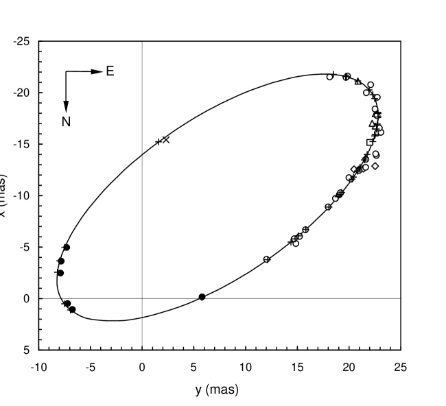
Figure 3: The orbit of $\beta$ Centauri. The data points are the SUSI results from Table 1 except for the MAPPIT point which is from Robertson et al. (1998). SUSI observations: 1997 $\diamondsuit$; 1998 $\triangle$; 1999 $\circ$; 2000 $\bullet$; 2002 $\sq$. MAPPIT observation: 1995 x. The points on the fitted orbit that correspond to the observational points are marked with $\large+$. Further details are given in the text.

Examination of Fig. 3 reveals that, while over most of the orbit the observational points are distributed on either side of the curve, the observations made in 2000 near to periastron all lie inside the fitted orbit. This is shown on an expanded scale in Fig. 4 where a section of the orbit close to periastron is plotted on an enlarged scale. While we have not been able to provide an explanation for this phenomenon we conjecture that, since the separation of the component stars is less than 7 stellar radii at periastron, the possibility of interaction may affect the brightness distributions such that the components appear closer than their centres of mass. Miroshnichenko et al. [2001] have reported interaction around periastron for the early B type binary $\delta$ Sco involving a Be outburst. Like $\beta$ Cen, $\delta$ Sco has a highly eccentric orbit, but with an orbital period of $\sim$ 10.6 years. Although $\delta$ Sco spends longer close to periastron, the closest approach is of the order of 30 times the primary radius compared with less than 7 radii for $\beta$ Cen. This suggests that some form of interaction is likely to occur.

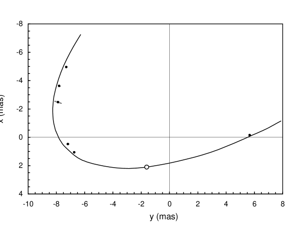
Figure 4: A section of the orbit of $\beta$ Centauri around periastron. The data points are the SUSI results from Table 1. Each point has its error ellipse plotted but, in all but one case, it is too small to extend outside the plotted point. The curve is the orbital fit shown in Fig. 3. The location of periastron is marked by a circle.

6 Combination of the Spectroscopic and Interferometric Results

The interferometric and spectroscopic results can be combined to yield the distance to the system, the absolute magnitudes of the components and the masses of the components. Not all the parameters are required for this purpose and the relevant parameters from the two techniques are summarised in Table 4. A mean of the interferometric and spectroscopic values for the eccentricity is adopted.

Table 4: Values of parameters for $\beta$ Cen determined directly by interferometry and spectroscopy and used to derive the basic physical parameters of the system.

Parameter	Value	Source
Period ($P$)	357$\aas@@fstack{d}$00$\pm$0$\aas@@fstack{d}$07	S
$K_{1}$ (km s-1)	63.8$\pm$0.6	S
$K_{2}$ (km s-1)	63.8$\pm$0.8	S
Eccentricity ($e$)	0.821$\pm$0.003	I + S
Angular semi-major axis ($a$)	0$\aas@@fstack{\prime\prime}$02532$\pm$0$\aas@@fstack{\prime\prime}$00023	I
Inclination ($i$)	67$\aas@@fstack{\circ}$4$\pm$0$\aas@@fstack{\circ}$3	I
Brightness ratio ($\beta$) (at $\lambda$442 nm)	0.868$\pm$0.015	I

As the two sets of data result in a single self-consistent set of parameters we are able to derive the masses of the components with high precision. Functions containing the masses of the primary (M₁) and secondary (M₂) components in solar mass units and the semi-major axis ($a$) of the orbit in AU are given by [1978]:

$$M_{1}\sin^{3}{i}=1.036\times 10^{-7}(K_{1}+K_{2})^{2}K_{2}P(1-e^{2})^{3/2},$$ (7)

$$M_{2}\sin^{3}{i}=1.036\times 10^{-7}(K_{1}+K_{2})^{2}K_{1}P(1-e^{2})^{3/2},$$ (8)

$$a\sin{i}=9.1919\times 10^{-5}(K_{1}+K_{2})P(1-e^{2})^{1/2}.$$ (9)

The values for these functions, computed from the data in Table 4, are listed in Table 5.

Table 5: Values of parameters for $\beta$ Cen derived from the parameters listed in Table 4 using equations (1)–(3). $M_{1}$ and $M_{2}$ are the masses of the primary and secondary respectively and $a$ is the semi-major axis of the orbit.

Parameter	Value	Reference
$M_{1}\sin^{3}{i}$ (M⊙)	7.15$\pm$0.24	Equ. (7)
$M_{2}\sin^{3}{i}$ (M⊙)	7.15$\pm$0.23	Equ. (8)
$a\sin{i}$ (AU)	2.391$\pm$0.032	Equ. (9)

6.1 The distance to $\beta$ Cen

The parallax of the system can also be determined by combining the interferometric and spectroscopic results and is given by:

$$\pi\arcsec=\frac{a\arcsec\sin{i}}{(a\sin{i})}$$ (10)

A parallax determined in this way has been appropriately termed an orbital parallax [1992]. Combining $a\arcsec$ and $i$ from Table 4 with $a\sin{i}$ from Table 5 gives the orbital parallax of $\beta$ Cen equal to 9.78$\pm$0.16 mas. This is to be compared with the HIPPARCOS parallax of 6.21$\pm$0.56 mas [1997]. There is a large and significant difference in spite of the relatively large fractional uncertainty in the HIPPARCOS value. The HIPPARCOS catalogue recognises $\beta$ Cen as a binary system but has no mention of the dual nature of the primary component of $\beta$ Cen and lists only the faint third magnitude companion. We conjecture that the HIPPARCOS value for the parallax is seriously affected by the binary nature of the primary of $\beta$ Cen. In fact, the HIPPARCOS observations of spectroscopic binaries were not fitted in general with an orbital model to derive the value for the parallax. While reprocessing of the HIPPARCOS astrometric data has been performed for many single-lined spectroscopic binaries (see for example [2003] and references therein), it has not been done for $\beta$ Cen. For this reason we adopt the value derived directly from the interferometric and spectroscopic data. The parallax we have adopted is equivalent to a distance of 102.3$\pm$1.7 pc.

6.2 The absolute magnitudes and spectral types of the components of $\beta$ Cen

Breger [1967] has given the following photometric data for $\beta$ Cen: V = 0.61, (B-V) = -0.24 and (U-B) = -0.99. Since the magnitude difference is only 0.15$\pm$0.02 at a wavelength of 442 nm (from the brightness ratio of 0.868$\pm$0.015 given in Table  4) and, as will be shown in Section 6.3, the masses of the components are equal, any difference in the colours of the two components will be very small and they will be assumed to be the same. Reddening will be small for this relatively nearby system (distance $\sim$ 102 pc) and E(B-V) is estimated to be $\sim$ 0.03. It follows that (B-V)₀ = -0.27 and we adopt A${}_{V}=0.09\pm 0.03$.

Using the parallax from Section 6.1 the absolute visual magnitude $M_{V}$ of the system is given by:

$$M_{V}=V-0.09-5.0\log(102.4/10).$$ (11)

Thus $M_{V}$ = -4.53$\pm$0.05 for the two components combined. The brightness ratio of 0.868$\pm$0.015, although measured at $\lambda$442 nm, is unlikely to differ significantly in the V band because of the equality of their masses and the small difference in luminosity between the two components. Assuming that the same brightness ratio is valid in the visual band, the absolute visual magnitudes for the two components are $M_{V\mathrm{primary}}=-3.85\pm 0.05$ and $M_{V\mathrm{secondary}}=-3.70\pm 0.05$.

These values for the absolute visual magnitudes lie between the values given by Balona & Crampton [1974] for spectral types B1 III (-4.1) and B2 III (-3.7) and are close to the value of -3.9 given by Schmidt-Kaler [1982] for B2 III. They lie in the middle of the range of absolute visual magnitudes for $\beta$ Cep stars [1993].

6.3 The masses of the components of $\beta$ Cen

The combination of the value for $i$ from Table 4 with the values for $M_{1}\sin^{3}{i}$ and $M_{2}\sin^{3}{i}$ from Table 5 gives the mass of the primary $M_{1}$ equal to 9.09$\pm$0.32 M_⊙. Similarly the mass of the secondary $M_{2}$ is 9.09$\pm$0.31 M_⊙. These are the most accurate mass estimates of any $\beta\,$Cep star in a binary system known to date.

Masses for early type giants are in general rather uncertain. The mass for a B0 III type star is usually taken as $\sim$ 20 M_⊙ and, for a B5 III type, $\sim$ 7 M_⊙ [1982]. The values we have determined for the components of $\beta$ Cen are significantly lower at B1 III than implied by those generally accepted for B giant stars.

Refined mass estimates at $\sim$3.5 per cent accuracy, which is the level of our results for $\beta\,$Cen, have recently become available for two single $\beta\,$Cep stars from asteroseismology, i.e. from detailed interpretation of the measured frequencies and mode identification of their oscillations. Such studies have led to very similar mass estimates for these two single stars, i.e. a mass range [9.0,9.5] M_⊙ for HD 129929 [2003] and [9.0,9.9] M_⊙ for $\nu\,$Eri [2004]. The mass of the eclipsing binary $\beta\,$Cep star 16 Lac is also rather well constrained and lies in [9.0,9.7] M_⊙ [2003].

The masses of all the known $\beta\,$Cep stars as a group of variables have mainly been derived from photometric calibrations, e.g. of the Walraven, Geneva and Strömgren systems. This method provided systematically too high masses for the three stars with accurate seismic mass determination: $M\simeq\,10$ to 11.3 M_⊙ for HD 129929; $M\simeq\,10$ to 10.8 M_⊙ for $\nu\,$Eri and $M=10\,$M_⊙ for 16 Lac (values taken from Heynderickx, Waelkens & Smeyers 1994; see also Sterken & Jerzykiewicz 1993) to be compared with the seismic values listed above. The situation is of course worse when we consider the mass estimates of photometric calibrations for spectroscopic binaries since the binarity is not usually taken into account in such global calibrations. Heynderickx et al. [1994], for example, list a mass between 14.4 and 15.2 M_⊙ from treating $\beta\,$Cen as a single star, as they did all other stars in their sample. Their estimate for the mass is far too high compared with our results. Since a large fraction of the $\beta\,$Cep stars turn out to be a member of a spectroscopic binary with not too different components (Aerts & De Cat 2003), it is unavoidable that the mass estimates of these group members from photometry are very unreliable.

Table 6: The parallax ($\pi$), masses ($M_{1}$ & $M_{2}$) and absolute visual magnitudes ($M_{1V}$ & $M_{2V}$) for $\beta$ Cen and its component stars. The absolute visual magnitudes were computed directly from the photometric data, the adopted parallax, and the brightness ratio $\beta$ given in Table 4.

Parameter	Value
$\pi$ (mas)	9.77$\pm$0.15
$M_{1}$ (M⊙)	9.09$\pm$0.31
$M_{2}$ (M⊙)	9.09$\pm$0.30
$M_{1V}$	-3.85$\pm$0.05
$M_{2V}$	-3.70$\pm$0.05

7 Summary

The orbital parameters for the primary component of $\beta$ Cen have been determined from interferometric observations made with SUSI. These parameters have been combined with the high resolution double-lined spectroscopic data for $\beta$ Cen reported in Ausseloos et al. [2002], the analysis of which has been revised here. The combination of data has yielded the masses and absolute visual magnitudes of the component stars and an accurate distance to the system. The very precise results of this powerful combination of techniques are summarised in Table 6.

The results presented in this paper constitute a very suitable starting point for any future asteroseismic modelling of $\beta\,$Cen’s two pulsating components. The star is also an ideal target to investigate possible tidal effects on the oscillations in view of the very close passage (less than 10 times the radii of the component stars) of the stars at periastron although, for this, long-term monitoring over several orbits is required.

8 Acknowledgements

The SUSI programme has been funded jointly by the Australian Research Council and the University of Sydney, with additional support from the Pollock Memorial Fund and the Science Foundation for Physics within the University of Sydney. The authors are grateful to Bill Hartkopf for making the binary orbit fitting program available to us and for assistance with its implementation. MA, CA and KU thank Petr Hadrava and Petr Harmanec for putting the FOTEL code at their disposal and acknowledge financial support from the Research Fund K.U.Leuven under grant GOA/2003/04.

References

- [2003] Aerts C., De Cat P., 2003, Space Science Rev., 105, 453
- [2003] Aerts C., Thoul A., Dasźynska J., Scuflaire R., Waelkens C., Dupret M-A., Niemczura E., Noels A., 2003, Science, 300, 1926
- [ 1992] Armstrong J. T. et al., 1992, AJ, 104, 241
- [2002] Ausseloos M., Aerts C., Uytterhoeven K., Schrijvers C., Waelkens C., Cuypers J., 2002, A&A, 384, 209
- [1996] Babu G. J., Feigelson E. D., 1996, Astrostatistics, Chapman & Hall, London
- [1974] Balona L., Crampton D., 1974, MNRAS, 166, 203
- [1967] Breger M., 1967, MNRAS, 136, 51
- [1996] Davis J., Tango W. J., 1996, PASP, 108, 456
- [1999a] Davis J., Tango W. J., Booth A. J., ten Brummelaar T. A., Minard R. A., Owens, S. M., 1999a, MNRAS, 303, 773
- [1999b] Davis J., Tango W. J., Booth A. J., Thorvaldson E. D., Giovannis J., 1999b, MNRAS, 303, 783 303, 783 303, 783
- [1997] ESA 1997, The Hipparcos and Tycho Catalogues, ESA SP-1200
- [1990] Hadrava P., 1990, Contr. Astron. Obs. Skalnate Pleso, Vol 20, 23
- [1967] Hanbury Brown R., Davis J., Allen L. R., 1967, MNRAS, 137, 375
- [1974] Hanbury Brown R., Davis J., Allen L. R., 1974, MNRAS, 167, 121
- [2004] Harmanec P., Uytterhoeven K., Aerts C., 2004, A&A, 422, 1013
- [1989] Hartkopf W. I., McAlister H. A., Franz O. G., 1989, AJ, 98, 1014
- [1978] Heintz W. D., 1978, Double Stars, Geophysics and Astrophysics Monographs, Vol. 15, Reidel, Dordrecht
- [1971] Herbison-Evans D., Hanbury Brown R., Davis J., Allen L. R., 1971, MNRAS, 151, 161
- [1994] Heynderickx D., Waelkens C., Smeyers P., 1994, A&AS, 105, 447
- [1982] Hoffleit D., 1982, The Bright Star Catalogue (Fourth Revised Edition), Yale University Observatory, New Haven
- [1894] Léhmann-Filhés R., 1894, Astr. Nach., 136, 17
- [1975] Lomb N. R., 1975, MNRAS, 172, 639
- [2001] Miroshnichenko A. S., et al., 2001, A&A, 377, 485
- [1965] Nelder J. A., Mead R., 1965, Computer Journal, 7, 308
- [2004] Pamyatnykh A. A., Handler G., Dziembowski W. A., 2004, MNRAS, 350, 1022
- [1997] Perryman M. A. C. et al., 1997, The Hipparcos Catalogue, A&A, 323, 49
- [2003] Pourbaix D., Boffin H. M. J., 2003, A&A, 398, 1163
- [1999] Robertson J. G., Bedding T. R., Aerts C., Waelkens C., Marson R. G., Barton J. R., 1999, MNRAS, 302, 245
- [1982] Schmidt-Kaler Th., in Landolt-Börnstein, Volume VI/2b, 1, Springer-Verlag, Berlin-Heidelberg, 1982
- [1968] Shobbrook R. R., Robertson J. W., 1968, PASA, 1, 82
- [1993] Sterken C., Jerzykiewicz M., 1993, Space Science Rev., 62, 95
- [1934] Struve O., Ebbighausen E., 1934, ApJ, 80, 365
- [1958] Struve O., Sahade J., Huang S-S., Zebergs V., 1958, ApJ, 128, 310
- [2003] Thoul A., Aerts C., Dupret M. A., Scuflaire R., Korotin S. A., Egorova I. A., Andrievsky S. M., Lehmann H., Briquet M., De Ridder, J., Noels A., 2003, A&A 406, 287
- [2004] Uytterhoeven, K., Willems B., Lefever K., Aerts C., Telting J. H., Kolb U., 2004, A&A, in press