The XMM-Newton view of PG quasars

We present results of a systematic analysis of the XMM–Newton spectra of 40 quasars (QSOs) (z$\leq 1.72$) from the Palomar–Green (PG) Bright Quasar Survey sample (M${}_{B}<-$23). The sample includes 35 radio-quiet quasars (RQQs) and 5 radio-loud quasars (RLQs). The analysis of the spectra above 2 keV reveals that the hard X–ray continuum emission can be modeled with a power law component with $\langle\Gamma_{2-12\leavevmode\nobreak\ keV}\rangle=1.89\pm 0.11$ and $\langle\Gamma_{2-12\leavevmode\nobreak\ keV}\rangle$ = 1.63${}^{+0.02}_{-0.01}$ for the RQQs and RLQs, respectively. Below 2 keV, a strong, broad excess is present in most QSO spectra. This feature has been fitted with four different models assuming several physical scenarios. All tested models (blackbody, multicolor blackbody, bremsstrahlung and power law) satisfactorily fitted the majority of the spectra. However, none of them is able to provide an adequate parameterization for the soft excess emission in all QSOs, indicating the absence of an universal shape for this spectral feature. An additional cold absorption component was required only in three sources. On the other hand, as recently pointed out by Porquet et al. (2004) for a smaller sample of PG QSOs, warm absorber features are present in  50% of the QSO spectra in contrast with their rare occurrence ($\sim$ 5–10%) found in previous studies. The XMM–Newton view of optically–selected bright QSOs therefore suggests that there are no significant difference in the X–ray spectral properties once compared with the low–luminosity Seyfert 1 galaxies. Properties of the Fe K$\alpha$ emission lines are presented in a companion paper.

1 Introduction

Quasars (QSOs) emit a large amount of their emission in the X–ray band, where luminosities can reach 10^46-47 erg s^-1 (Zamorani et al. 1981). Variability studies indicate that the X–rays originated in a region very close to the central object, probably an accreting supermassive black hole. Therefore, the analysis of the emission in this energy range provides strong constraints for models of the mechanism powering the QSOs. X–ray emission properties of QSOs have been largely studied during the last decades. Different samples of QSOs have been analyzed with previous X–ray satellites such as Einstein (Zamorani et al. 1981), EXOSAT (Comastri et al. 1992), Ginga (Lawson & Turner 1997), ASCA (Cappi et al. 1997; George et al. 2000; Reeves & Turner 2000), ROSAT (Schartel et al. 1997; Laor et al. 1997) and BeppoSAX (Mineo et al. 2000).

From these studies it emerges that the typical spectrum of a QSO in the hard ($>$2 keV) band is dominated by a power law–like emission with a photon index $\Gamma\sim 2$. For Seyfert galaxies, the most popular physical scenario (Haardt & Maraschi 1991) explains this hard spectral component as the emission originating in a hot corona placed above the accretion disk which comptonizes the UV-soft X–ray thermal emission from the disk and up-scatters it into the hard X–ray band. Part of the continuum emission is then reprocessed in the disk and/or in other nuclear physical components (i.e. the molecular torus, clouds) producing the typical reflection spectrum (George & Fabian 1991). The most striking feature in the reflection spectrum is the fluorescent Fe K$\alpha$ emission line around 6.4 keV. This scenario has been also extended to the QSOs, although the observational evidences of a reflection component in their X–ray spectra are poor. Signatures of the presence of large amounts of ionized and/or cold gas were also detected in the soft X-ray portion of QSO spectra (Cappi et al. 1997; George et al. 1997). It has been reported as well that a fraction of QSOs present a gradual upturn in the emission emerging below 2-3 keV, the so-called soft excess (Comastri et al. 1992), whose nature is still debated.

Systematic analysis of QSOs with high spectral resolution provide a very useful tool in order to investigate their nature. In this paper we analyze a sample of QSOs observed with XMM–Newton, which provides the highest throughput and sensitivity to date. We investigate the spectral characteristics of the objects in the sample and search for common features in order to elucidate the physical mechanisms responsible for the X–ray emission. The sample includes both radio loud and radio quiet quasars (RLQs and RQQs, respectively). The classification is based on the strength of the radio emission relative to the optical one. Many studies show systematic differences in the spectral properties in the X–ray band of both types of objects, as for instance the slope of the power law (Laor et al. 1997; Reeves & Turner 2000) which is evidence for a possible difference in the physical processes which give rise the X–ray emission. Therefore the chosen sample allows to provide useful information about possible differences between RLQs and RQQs. Results based on XMM–Newton observations of a smaller subsample of PG QSOs have been recently presented by Porquet et al. (2004; P04 hereafter). Thanks to the larger number of objects, our survey allows to obtain a complete description of the X–ray spectral properties of optically–selected QSOs based on a sounder statistical ground.

In Sect. 2 we present the general characteristics of the objects included in the sample, as well as the XMM–Newton observations and the applied reduction technique. We performed a systematic analysis of all objects assuming several physical scenarios for the emission of the QSO. The corresponding results are presented in Sect. 3, which also includes a detailed analysis of the most peculiar objects. In Sect. 4 we discuss observational constraints obtained by this study to the physical scenario for the X–ray emission/absorption mechanisms at work in QSOs and we also compare them with previous similar works. Finally, the main results of this study are summarized in Sect. 5.

2 XMM–Newton observations

2.1 The sample

The present sample is constituted by all Palomar–Green (PG) quasars (Schmidt & Green 1983) with available EPIC observations in the XMM–Newton Science Archive (XSA) as of February 2004 plus PG 1001$+$054, yielding a preliminary sample of 42 objects. Two QSOs (0003$+$199 and 1426$+$015) were excluded from the present study since all their EPIC exposures are affected by pile–up. Basic data for the final sample of 40 objects (i.e. name, coordinates, redshifts and the line–of–sight Galactic column density) are given in Table 1. The redshifts span values from 0.036 to 1.718. All but 5 QSOs (0007$+$106, 1100$+$772, 1226$+$023, 1309$+$355, 1512$+$370, i.e. $\sim$13% of the sample) are radio–quiet sources according to the definition proposed in Kellermann et al. (1994) i.e. exhibit a ratio of radio to optical emission $R_{L}$ $\leq$ 10. It is worth noting that our sample includes all but two (1425$+$267 and 1543$+$489) of the sources in the complete sample studied in Laor et al. (1997) (i.e. all the PG QSOs with $M_{B}<-$23, $z\leq$ 0.4 and N${}_{\rm H}^{\rm Gal}$ $<$ 1.9 $\times$ 10²² cm^-2).

Table 1: The Sample

PG Name	Other name	RA	Dec	z	N${}^{\rm Gal}_{H}$
		(J2000)	(J2000)		(10${}^{20}\,{\rm cm^{-2}}$)
0007$+$106⋆	III Zw 2	00 10 31.0	$+$10 58 30	0.089	6.09a
0050$+$124	I Zw 1	00 53 34.9	$+$12 41 36	0.061	4.99a
0157$+$001	MKN 1014	01 59 50.2	$+$00 23 41	0.163	2.46b
0804$+$761	1H 0758$+$762	08 10 58.6	$+$76 02 42	0.100	3.26c
0844$+$349	TON 914	08 47 42.4	$+$34 45 04	0.064	3.32c
0947$+$396L		09 50 48.4	$+$39 26 50	0.206	1.92b
0953$+$414L		09 56 52.1	$+$41 15 34	0.239	1.12c
1001$+$054L		10 04 20.1	$+$05 13 00	0.161	1.88a
1048$+$342L		10 51 43.8	$+$33 59 26	0.167	1.75b
1100$+$772⋆	3C 249.1	11 04 13.7	$+$76 58 58	0.312	3.17e
1114$+$445L		11 17 06.4	$+$44 13 33	0.144	1.93b
1115$+$080		11 18 16.0	$+$07 45 59	1.718	3.62b
1115$+$407L		11 18 30.2	$+$40 25 53	0.154	1.74b
1116$+$215L	TON 1388	11 19 08.6	$+$21 19 18	0.177	1.44a
1202$+$281L		12 04 42.1	$+$27 54 11	0.165	1.72d
1206$+$459		12 08 58.0	$+$45 40 35	1.158	1.31d
1211$+$143		12 14 17.7	$+$14 03 13	0.081	2.76c
1216$+$069L		12 19 20.9	$+$06 38 38	0.334	1.57c
1226$+$023L⋆	3C 273	12 29 06.7	$+$02 03 08	0.158	1.89d
1244$+$026		12 46 35.3	$+$02 22 09	0.048	1.93a
1307$+$085		13 09 47.0	$+$08 19 48	0.155	2.11d
1309$+$355L⋆	TON 1565	13 12 17.8	$+$35 15 21	0.184	1.00b
1322$+$659L		13 23 49.5	$+$65 41 48	0.168	1.89b
1352$+$183L		13 54 35.6	$+$18 05 17	0.158	1.84a
1402$+$261L		14 05 16.2	$+$25 55 35	0.164	1.42a
1404$+$226		14 06 21.8	$+$22 23 35	0.095	3.22a
1407$+$265		14 07 07.8	$+$26 32 30	0.940	1.38a
1411$+$442L		14 13 48.3	$+$44 00 14	0.0896	1.05c
1415$+$451L		14 17 01.24	$+$44 56 16	0.114	1.10e
1427$+$480L		14 29 43.0	$+$47 47 26	0.221	1.69b
1440$+$356L	MKN 478	14 42 07.4	$+$35 26 23	0.079	0.97b
1444$+$407L		14 46 45.9	$+$40 35 05	0.267	1.27e
1501$+$106	MKN 841	15 04 01.2	$+$10 26 16	0.036	2.19b
1512$+$370L⋆	4C $+$37.43	15 14 43.0	$+$36 50 50	0.371	1.36e
1613$+$658	MKN 876	16 13 57.2	$+$65 43 09	0.129	2.66a
1626$+$554L		16 27 56.0	$+$55 22 31	0.133	1.55b
1630$+$377		16 32 01.2	$+$37 37 49	1.466	0.90a
1634$+$706		16 34 31.4	$+$70 31 34	1.334	5.74a
2214$+$139	MKN 304	22 17 11.5	$+$14 14 28	0.066	4.96d
2302$+$029		23 04 45.0	$+$03 11 46	1.044	5.27d

^⋆ Radio–loud objects. ^L Objects included in Laor et al. (1997) References for N_H values: ^a Elvis, Lockman & Wilkes (1989); ^b Murphy et al. (1996); ^c Lockman & Savage (1995); ^d Dickney & Lockman (1990); ^e Stark et al. (1992).

2.2 Data reduction

The raw data from the EPIC instruments were processed using the standard Science Analysis System (SAS) v5.4.1 (Loiseau 2003) to produce the linearized event files for pn, MOS1  and MOS2. Only events with single and double patterns for the pn (PATTERN $\leq$ 4) and single, double, triple and quadruple events for the MOS (PATTERN $\leq$ 12), were used for the spectral analysis. The subsequent event selection was performed taking into account the most updated calibration files at the time of the reduction (September 2003). All known flickering and bad pixels were removed. Furthermore, periods of background flaring in the EPIC data were excluded using the method described in Piconcelli et al. (2004). Useful exposure times after cleaning are listed in Table 2 for each camera together with the date and the revolution of each reduced observation. In the case of 0844$+$349, 1244$+$026 and 1440$+$356, the pn observations are affected by pile–up and, therefore, only the MOS spectra were used for the analysis. On the other hand, for 1226$+$023 and 1501$+$106 only pn data were analyzed due to impossibility to select a background region since the MOS  observations were carried out in small window mode. Source spectra were extracted from circular regions centered on the peak of the X-ray counts. Backgrounds were estimated in a source–free circle of equal radius close to the source on the same CCD. Appropriate response and ancillary files for both the pn and the MOS cameras were created using the RMFGEN and ARFGEN tools in the $SAS$ software, respectively. As the difference between the MOS1 and MOS2 response matrices are a few percent, we created a combined MOS spectrum and response matrix. The background–subtracted spectra for the pn and combined MOS cameras were then simultaneously fitted. According to the current calibration uncertainties we performed the spectral analysis in the 0.3-12 keV band for pn and in the 0.6–10 keV band for the MOS cameras, respectively.

Table 2: Journal of Observations.

PG Name	Date	Rev.	Exposure Time (ks)			PG Name	Date	Rev.	Exposure Time (ks)
			pn	MOS1	MOS2				pn	MOS1	MOS2
0007$+$106	2000–07–04	104	9.9	7.5	7.5	1307$+$085	2002–06–13	460	11.2	13.3	13.3
0050$+$124	2002–06–22	464	18.6	20.7	19.6	1309$+$355	2002–06–10	458	25.2	28.4	27.3
0157$+$001	2000–07–29	117	10.1	10.4	10.4	1322$+$659	2002–05–11	443	8.6	11.4	11.6
0804$+$761	2000–11–04	166	0.5	6.6	6.5	1352$+$183	2002–07–20	478	12.3	14.7	14.9
0844$+$349	2000–11–04	166	-	23.3	23.3	1402$+$261	2002–01–27	391	9.1	11.9	11.9
0947$+$396	2001–11–03	349	17.5	20.9	21.1	1404$+$226	2001–06–18	279	16.3	19.4	18.1
0953$+$414	2001–11–22	358	11.5	12.4	14.7	1407$+$265	2001–12–22	373	35.1	36.8	36.9
1001$+$054	2003–05–04	623	8.8	10.1	11.0	1411$+$442	2002–07–10	473	23.1	35.4	35.4
1048$+$342	2002–05–13	444	28.1	32.1	32.1	1415$+$451	2002–12–08	549	21.1	24.1	24.1
1100$+$772	2002–11–01	530	19.2	22.5	22.5	1427$+$480	2002–05–31	453	35.2	38.9	38.5
1114$+$445	2002–05–14	445	37.7	42.2	42.3	1440$+$356	2001–12–23	373	-	28.2	24.8
1115$+$080	2001–11–25	360	53.8	61.8	61.8	1444$+$451	2002–08–11	489	18.5	21.0	21.0
1115$+$407	2002–05–17	446	15	20.2	19.9	1501$+$106	2001–01–14	201	9.4	-	-
1116$+$215	2001–12–02	363	5.5	8.3	8.4	1512$+$370	2002–08–25	496	17.6	20.4	20.4
1202$+$281	2002–05–30	453	12.9	17.3	17.3	1613$+$658	2001–04–13	246	3.5	3.3	3.5
1206$+$459	2002–05–11	443	9.1	12.2	12.2	1626$+$554	2002–05-05	440	5.5	8.7	7.2
1211$+$143	2001–06–15	278	49.5	53.4	53.3	1630$+$377	2002–01–06	380	12.3	15.7	16
1216$+$069	2002–12–18	554	14	16.5	16.5	1634$+$706	2002–11–22	541	15.7	19.0	18.8
1226$+$023	2000–06–15	95	20.8	$-$	$-$	2214$+$139	2002–05–12	444	29	33.4	35.5
1244$+$026	2001–06–17	279	-	12.1	12.1	2302$+$029	2001–11–29	362	9.0	12.4	12.2

3 Analysis of the spectra

The source spectra were grouped such that each spectral bin contains at least 35 (or more in the case of the brightest sources) counts in order to apply the modified $\chi^{2}$ minimization technique and they were analyzed using XSPEC v.11.2 (Arnaud 1996). Galactic absorption (see Table 1) is always implicitly included in all the spectral models presented hereafter. The photoelectric absorption cross sections of Morrison & McCammon (1983) and the solar abundances of Anders & Grevesse (1989) were used. The quoted errors refer to the 90% confidence level for one interesting parameter (i.e. $\Delta\chi^{2}$ = 2.71; Avni 1976). Throughout this paper we assume a flat $\Lambda$CDM cosmology with ($\Omega_{\rm M}$,$\Omega_{\rm\Lambda}$) = (0.3,0.7) and a Hubble constant of 70 km s^-1 Mpc^-1 (Bennett et al. 2003). All fit parameters are given in the quasar rest frame.

Table 3: Spectral fitting results. I: Power law model applied to the hard band (2–12 keV). 1001$+$054 is excluded due to the very poor statistics in this energy range.

PG Name	$\Gamma_{\rm 2-12}$	$\chi^{2}$	dof	PG Name	$\Gamma_{\rm 2-12}$	$\chi^{2}$	dof
0007$+$106	1.61${}^{+0.05}_{-0.04}$	135	179	1307$+$085	1.46${}^{+0.07}_{-0.08}$	117	92
0050$+$124	2.28${}^{+0.03}_{-0.03}$	276	266	1309$+$355	1.72${}^{+0.07}_{-0.06}$	95	87
0157$+$001	2.1${}^{+0.2}_{-0.2}$	31	48	1322$+$659	2.2${}^{+0.2}_{-0.2}$	91	88
0804$+$761	2.05${}^{+0.07}_{-0.07}$	148	135	1352$+$183	1.91${}^{+0.09}_{-0.09}$	126	97
0844$+$349	2.11${}^{+0.05}_{-0.05}$	106	109	1402$+$261	2.06${}^{+0.09}_{-0.08}$	77	92
0947$+$396	1.81${}^{+0.06}_{-0.06}$	121	137	1404$+$226	2.3${}^{+0.8}_{-0.8}$	5	9
0953$+$414	2.01${}^{+0.07}_{-0.06}$	64	69	1407$+$265	2.19${}^{+0.07}_{-0.07}$	83	118
1001$+$054	$-$	$-$	$-$	1411$+$442	0.38${}^{+0.11}_{-0.13}$	111	67
1048$+$342	1.77${}^{+0.05}_{-0.05}$	113	149	1415$+$451	2.03${}^{+0.08}_{-0.08}$	65	105
1100$+$772	1.65${}^{+0.05}_{-0.05}$	180	220	1427$+$480	1.90${}^{+0.07}_{-0.05}$	115	155
1114$+$445	1.48${}^{+0.04}_{-0.03}$	255	241	1440+356	2.03${}^{+0.06}_{-0.07}$	173	104
1115$+$080	2.00${}^{+0.11}_{-0.11}$	87	87	1444$+$407	2.12${}^{+0.12}_{-0.12}$	30	48
1115$+$407	2.16${}^{+0.07}_{-0.07}$	94	100	1501$+$106	1.88${}^{+0.03}_{-0.03}$	164	154
1116$+$215	2.14${}^{+0.08}_{-0.08}$	105	106	1512$+$370	1.82${}^{+0.06}_{-0.07}$	97	130
1202$+$281	1.69${}^{+0.05}_{-0.05}$	189	195	1613$+$658	1.70${}^{+0.10}_{-0.10}$	48	66
1206$+$459	2.0${}^{+0.4}_{-0.5}$	15	12	1626$+$554	1.95${}^{+0.10}_{-0.10}$	130	137
1211$+$143	1.76${}^{+0.03}_{-0.03}$	380	278	1630$+$377	2.2${}^{+0.2}_{-0.4}$	17	10
1216$+$069	1.73${}^{+0.08}_{-0.10}$	54	79	1634$+$706	2.04${}^{+0.09}_{-0.09}$	79	84
1226$+$023	1.634${}^{+0.009}_{-0.009}$	260	193	2214$+$139	0.94${}^{+0.04}_{-0.04}$	469	256
1244$+$026	2.55${}^{+0.11}_{-0.11}$	69	55	2302$+$029	$2.2^{+0.3}_{-0.2}$	13	23

3.1 Continuum emission above 2 keV

A simple redshifted power law model has been fitted to the hard X-ray band, excluding the data below 2 keV where additional spectral components like soft excess and absorbing features can heavily modify the primary source continuum. Such a fit resulted acceptable for most sources, with only five objects (i.e. 1211$+$143, 1226$+$023, 1411$+$442, 1630$+$377 and 2214$+$139) yielding an associate $\chi^{2}_{\nu}$ $>$ 1.2. Some of these sources show a very flat spectrum with $\Gamma_{2-12}$ $<$ 1 which suggests the presence of intrinsic absorption obscuring the primary continuum. The resulting best–fit parameters are displayed in Table 3. Using the maximum likelihood technique (see Maccacaro et al. 1988), we have calculated the best simultaneous estimate of the average photon index of $\langle\Gamma_{2-12}\rangle$ and the intrinsic spread $\sigma(\Gamma_{2-12})$. Figure 1 shows the 68%, 90% and 99% confidence contours for the two parameters together with the best-fit values obtained, i.e. $\langle\Gamma_{2-12}\rangle$ = $1.87^{+0.09}_{-0.10}$ and $\sigma(\Gamma_{2-12})$ = 0.36${}^{+0.08}_{-0.06}$ (errors have been calculated using the 68% contour level).

Figure 1: Confidence contours for the simultaneous determination of the photon index $\langle\Gamma_{2-12}\rangle$ and the intrinsic dispersion $\sigma(\Gamma_{2-12})$ together with the best-fit values found.

Table 4: Spectral fitting results. II: Power law model (Model PL) applied to the 0.3–12 keV band.

PG Name	$\Gamma$	Apl	$\chi^{2}$	d.o.f.	PG Name	$\Gamma$	Apl	$\chi^{2}$	d.o.f.
0007$+$106	1.82${}^{+0.01}_{-0.02}$	2.32${}^{+0.02}_{-0.02}$ $\times$ 10-2	407	307	1307$+$085	$1.76^{+0.04}_{-0.02}$	5.5 ${}^{+0.2}_{-0.2}\times 10^{-4}$	781	214
0050$+$124	$1.77^{+0.02}_{-0.02}$	$1.60^{+0.02}_{-0.02}\times 10^{-3}$	1359	394	1309$+$355	1.94${}^{+0.02}_{-0.03}$	3.01${}^{+0.05}_{-0.05}$ $\times$ 10-4	615	220
0157$+$001	$2.50^{+0.03}_{-0.03}$	$8.51^{+0.13}_{-0.13}\times 10^{-4}$	183	168	1322$+$659	2.81${}^{+0.02}_{-0.02}$	1.64${}^{+0.01}_{-0.01}$ $\times$ 10-3	515	216
0804$+$761	2.28${}^{+0.01}_{-0.02}$	7.21${}^{+0.07}_{-0.07}$ $\times$ 10-3	364	266	1352$+$183	$2.50^{+0.02}_{-0.02}$	$1.596^{+0.015}_{-0.015}\times 10^{-3}$	472	248
0844$+$349	$2.41^{+0.01}_{-0.01}$	$3.80^{+0.04}_{-0.04}\times 10^{-3}$	451	166	1402$+$261	$2.71^{+0.02}_{-0.02}$	2.10 ${}^{+0.02}_{-0.02}\times 10^{-3}$	449	219
0947$+$396	$2.307^{+0.016}_{-0.016}$	$1.341^{+0.012}_{-0.012}\times 10^{-3}$	496	265	1404$+$226	4.18${}^{+0.05}_{-0.05}$	2.20${}^{+0.07}_{-0.07}$ $\times$ 10-4	570	79
0953$+$414	2.46${}^{+0.01}_{-0.01}$	3.03${}^{+0.01}_{-0.01}$ $\times$ 10-3	823	290	1407$+$265	2.28${}^{+0.02}_{-0.02}$	2.00${}^{+0.03}_{-0.03}$ $\times$ 10-3	243	246
1001$+$054	4.0${}^{+0.4}_{-0.4}$	1.7${}^{+0.2}_{-0.2}$ $\times$ 10-5	156	10	1411$+$442	2.6${}^{+0.1}_{-0.1}$	5.0${}^{+0.2}_{-0.2}$ $\times$ 10-5	730	108
1048$+$342	2.24${}^{+0.02}_{-0.02}$	8.50${}^{+0.08}_{-0.08}$ $\times$ 10-4	559	275	1415$+$451	$2.55^{+0.02}_{-0.02}$	$8.49^{+0.08}_{-0.08}\times 10^{-4}$	458	232
1100$+$772	2.01${}^{+0.01}_{-0.01}$	2.16${}^{+0.01}_{-0.02}$ $\times$ 10-3	606	348	1427$+$480	$2.36^{+0.014}_{-0.014}$	$8.13^{+0.07}_{-0.07}\times 10^{-4}$	555	283
1114$+$445	1.14${}^{+0.01}_{-0.01}$	2.90${}^{+0.05}_{-0.05}$ $\times$ 10-4	3607	368	1440$+$356	$2.65^{+0.02}_{-0.02}$	3.09${}^{+0.03}_{-0.02}\times 10^{-3}$	731	161
1115$+$080	$1.77^{+0.02}_{-0.02}$	$6.3^{+0.2}_{-0.2}\times 10^{-4}$	354	214	1444$+$407	$2.72^{+0.03}_{-0.03}$	8.14 ${}^{+0.10}_{-0.10}\times 10^{-4}$	357	168
1115$+$407	2.72${}^{+0.02}_{-0.02}$	1.49${}^{+0.02}_{-0.02}$ $\times$ 10-3	530	234	1501$+$106	$2.47^{+0.02}_{-0.02}$	9.38 ${}^{+0.04}_{-0.04}\times 10^{-3}$	2281	225
1116$+$215	$2.60^{+0.02}_{-0.02}$	$3.45^{+0.03}_{-0.03}\times 10^{-3}$	456	234	1512$+$370	2.15${}^{+0.01}_{-0.02}$	1.49${}^{+0.01}_{-0.01}$ $\times$ 10-3	452	257
1202$+$281	$1.69^{+0.05}_{-0.05}$	$1.16^{+0.08}_{-0.08}\times 10^{-3}$	730	323	1613$+$658	2.13${}^{+0.04}_{-0.04}$	1.82${}^{+0.04}_{-0.04}$ $\times$ 10-3	354	184
1206$+$459	1.74${}^{+0.09}_{-0.09}$	2.4${}^{+0.2}_{-0.2}$ $\times$ 10-4	40	42	1626$+$554	2.25${}^{+0.02}_{-0.02}$	1.95${}^{+0.05}_{-0.05}$ $\times$ 10-3	345	271
1211$+$143	$3.14^{+0.02}_{-0.02}$	1.72${}^{+0.02}_{-0.03}\times 10^{-3}$	15193	404	1630$+$377	2.25${}^{+0.07}_{-0.07}$	5.2${}^{+0.4}_{-0.4}$ $\times$ 10-4	70	61
1216$+$069	2.19${}^{+0.03}_{-0.03}$	1.0${}^{+0.1}_{-0.2}$ $\times$ 10-3	336	204	1634$+$706	$2.22^{+0.08}_{-0.02}$	$3.57^{+0.09}_{-0.09}\times 10^{-3}$	238	210
1226$+$023	1.86${}^{+0.01}_{-0.01}$	2.85${}^{+0.01}_{-0.01}$ $\times$ 10-2	6455	264	2214$+$139	0.58${}^{+0.02}_{-0.02}$	1.34${}^{+0.03}_{-0.03}$ $\times$ 10-4	2483	367
1244$+$026	$2.90^{+0.02}_{-0.02}$	3.15${}^{+0.04}_{-0.04}\times 10^{-3}$	233	112	2302$+$029	$2.29^{+0.06}_{-0.06}$	$6.7^{+0.4}_{-0.4}\times 10^{-4}$	94	68

(^†) Flux at 1 keV in units of photons/keV/cm²/s.

Although the quality of the fit in the 2-12 keV band is good for most quasars, the residuals show an excess around 6 keV which suggests iron fluorescence emission. A detailed analysis of the Fe K$\alpha$ emission line is deferred to a second paper (see Jimenez-Bailon et al. 2004; Paper II hereafter).

3.2 Systematic modeling of the 0.3–12 keV continuum

The extrapolation of the power law to energies lower than 2 keV clearly revealed the presence of large deviations in all but one (i.e. 1206$+$459) spectra, with the most common residual feature being a smooth excess of soft X-ray flux. On the other hand, a handful of objects (i.e. 1001$+$054, 1114$+$445, 1115$+$080 and 2214$+$139) exhibit a deep and sharp deficit in the 0.5–2 keV band likely due to complex absorption.

3.2.1 Power law fit

The 0.3–12 keV spectrum of each source was fitted with a single power law model (PL) in order to provide an overall indication of the X–ray broad–band spectral shape ($\langle\Gamma_{0.3-12}\rangle$ = 2.30$\pm 0.15$ and dispersion of $\sigma(\Gamma_{0.3-12})$ = 0.60${}^{+0.12}_{-0.09}$). The vast majority of $\chi^{2}_{\nu}$ values associated with this parameterization show that it yields a very poor description of the EPIC data (see Table 4 for the results). This fact is an evident consequence of the inclusion of the 0.3–2 keV range in the fit, which is dominated by the emission of the steeper “soft excess” component. Therefore, we fitted more complex models accounting for the soft excess (Sect. 3.2) and the absorption features (Sect. 3.4) if present in the spectrum. The presence of iron emission lines is investigated in Paper II.

3.2.2 Soft excess modeling

We accounted for the soft excess emission by means of four different two–component continua: (A) blackbody (BBODY in XSPEC)$+$ power law; (B) multicolor blackbody (DISKBB in XSPEC) $+$ power law; (C) bremsstrahlung (BREMSS in XSPEC) $+$ power law; (D) power law $+$ power law. In Fig. 2 are plotted some examples of source spectra fitted with the above models which can be considered representative of the different shapes of soft excess emission found in the sample.

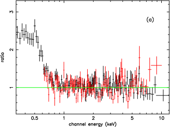
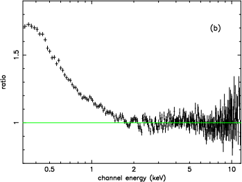
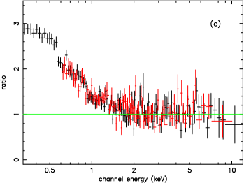
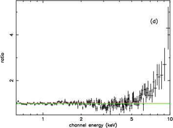
Figure 2: The ratios (data/model) resulting from fitting a power law to the 2-12 keV EPIC data (pn data in black, MOS in red) and extrapolating to lower energies (from top-left) in the case of the QSO (from top-left) (a) 1307+085 ($z$ = 0.155): the soft excess emission in this source results to be best–fitted with a blackbody (i.e. model A; see Table 10); (b) 1226+023 ($z$ = 0.158): note the broader excess than in 1307+085 (the two QSOs have a similar $z$) which requires two blackbodies (i.e. model E; see Table 10) to be parametrized; (c) 1352+183 ($z$ = 0.158) for which model C (i.e. bremsstrahlung $+$ power law) gives the best fit. Bottom-right: (d) the ratio resulted fitting with model A the EPIC data of 1440+356 ($z$ = 0.079). Note the large residuals at high energies. This QSO is best–fitted with a double power law model (i.e. model D; see Table 10).

Furthermore, photoelectric absorption edges were added to the fits whenever appropriate. We included these additional components by the $F-test$ criterion at a significance level $\geq$95%. For the high–$z$ QSO 1206$+$459, whose emission did not show any deviation from a simple power law continuum, we did not perform any further spectral fits. Eight sources (i.e. 0050$+$124, 1001$+$054, 1114$+$445, 1115$+$080, 1226$+$023, 1404$+$226, 1411$+$442, and 2214$+$139) exhibited spectra more complex than a two–component continuum (plus absorption edge) and yielded a $\chi^{2}_{\nu}$ $\geq$1.2 for each of the tested models. They are not listed in the relative Tables, but rather they are individually discussed in Sect. 3.4.

The best–fitting parameters resulted by the application of model A, B, C and D are shown in Table 5, 6, 7 and  8, respectively.

Table 5: Spectral fitting results. III: Power law plus blackbody model for the soft excess component (Model A).

PG Name	A${}^{{\dagger}}_{pl}$	$\Gamma$	A${}^{{\dagger}}_{BB}$	kT	Edge	$\tau$	$P_{F-test}$	$\chi^{2}_{\nu}$	dof
			($\times 10^{-5}$)	(keV)	(keV)		(%)
0007$+$106	1.97${}^{+0.07}_{-0.07}$ $\times$10-3	1.67${}^{+0.02}_{-0.02}$	1.5${}^{+0.2}_{-0.2}$	0.16${}^{+0.09}_{-0.09}$	$-$	$-$	$-$	318	305
0157+001	$7.1^{+0.5}_{-0.5}\times 10^{-4}$	$2.24^{+0.06}_{-0.07}$	1.0${}^{=}_{-}0.2$	$0.127^{+0.010}_{-0.010}$	$-$	$-$	$-$	149	166
0804$+$761	6.6${}^{+0.2}_{-0.1}$ $\times$ 10-3	2.18${}^{+0.02}_{-0.04}$	5.6${}^{+1.6}_{-1.3}$	0.112${}^{+0.013}_{-0.013}$	$-$	$-$	$-$	309	264
0844+349	$3.31^{+0.08}_{-0.08}\times 10^{-3}$	2.24${}^{+0.03}_{-0.03}$	7.0${}^{+2}_{-1}$	$0.108^{+0.008}_{-0.008}$	$-$	$-$	$-$	189	164
0947+396	$1.01^{+0.04}_{-0.05}\times 10^{-3}$	1.99${}^{+0.04}_{-0.04}$	2.0${}^{+0.2}_{-0.3}$	$0.160^{+0.007}_{-0.008}$	$0.75^{+0.02}_{-0.03}$	$0.28^{+0.07}_{-0.08}$	$>$99.9	254	261
0953$+$414	2.21${}^{+0.07}_{-0.07}$$\times$ 10-3	2.12${}^{+0.02}_{-0.04}$	5.5${}^{+0.4}_{-0.4}$	0.16 ${}^{+0.04}_{-0.04}$	0.73${}^{+0.02}_{-0.02}$	0.33${}^{+0.05}_{-0.05}$	$>$99.9	340	286
1048$+$342	6.5${}^{+0.2}_{-0.2}$ $\times$ 10-4	1.93${}^{+0.03}_{-0.03}$	1.15${}^{+0.09}_{-0.09}$	0.133 ${}^{+0.05}_{-0.05}$	$-$	$-$	$-$	283	273
1100$+$772	1.83${}^{+0.02}_{-0.05}$ $\times$ 10-3	1.84${}^{+0.03}_{-0.02}$	1.87${}^{+0.20}_{-0.20}$	0.141${}^{+0.008}_{-0.010}$	$-$	$-$	$-$	401	346
1116+215	$2.8^{+0.1}_{-0.1}\times 10^{-4}$	$2.29^{+0.04}_{-0.03}$	$6.0^{+0.5}_{-0.6}$	$0.113^{+0.005}_{-0.006}$	$-$	$-$	$-$	220	232
1202+281	$1.37^{+0.05}_{-0.05}\times 10^{-3}$	$1.80^{+0.03}_{-0.03}$	$2.7^{+0.2}_{-0.2}$	$0.159^{+0.007}_{-0.007}$	$0.72^{+0.02}_{-0.02}$	$0.33^{+0.07}_{-0.07}$	$>$99.9	328	319
1211+143	$9.6^{+0.3}_{-0.2}\times 10^{-4}$	$1.715^{+0.010}_{-0.012}$	$9.36^{+0.12}_{-0.17}$	$0.1157^{+0.0013}_{-0.0015}$	$0.771^{+0.012}_{-0.005}$	$0.35^{+0.04}_{-0.03}$	$>$99.9	771	400
					$0.953^{+0.02}_{-0.008}$	$0.28^{+0.03}_{-0.03}$	$>$99.9	571	398
					$7.28^{+0.16}_{-0.12}$	$0.54^{+0.09}_{-0.09}$	$>$99.9	458	396
1216$+$069	7.8${}^{+0.3}_{-0.4}$ $\times$ 10-4	1.91${}^{+0.05}_{-0.05}$	1.4${}^{+0.2}_{-0.2}$	0.13${}^{+0.01}_{-0.01}$	$-$	$-$	$-$	181	202
1244+026	$2.17^{+0.09}_{-0.08}\times 10^{-3}$	2.48${}^{+0.03}_{-0.03}$	4.93${}^{+0.04}_{-0.04}$	$0.16^{+0.01}_{-0.01}$	$-$	$-$	$-$	125	110
1307+085	$4.4^{+0.2}_{-0.2}\times 10^{-4}$	$1.50^{+0.04}_{-0.04}$	$1.2^{+0.1}_{-0.1}$	0.13${}^{+0.01}_{-0.01}$	$0.74^{+0.02}_{-0.02}$	$0.54^{+0.10}_{-0.14}$	99.9	232	210
1309$+$355	2.76${}^{+0.12}_{-0.12}$ $\times$ 10-4	1.80${}^{+0.04}_{-0.05}$	0.53${}^{+0.14}_{-0.10}$	0.104${}^{+0.008}_{-0.008}$	0.74${}^{+0.04}_{-0.02}$	0.4${}^{+0.2}_{-0.2}$	$>$99.9	238	216
1402+261	$1.58^{+0.08}_{-0.07}\times 10^{-3}$	$2.33^{+0.05}_{-0.05}$	$4.2^{+0.5}_{-0.4}$	$0.135^{+0.003}_{-0.004}$	$0.68^{+0.04}_{-0.05}$	$0.24^{+0.08}_{-0.08}$	99.8	243	215
1407$+$265	1.82${}^{+0.07}_{-0.07}$ $\times$ 10-3	2.21${}^{+0.03}_{-0.03}$	0.7${}^{+0.3}_{-0.3}$	0.20${}^{+0.03}_{-0.03}$	$-$	$-$	$-$	223	244
1415+451	$6.4^{+0.3}_{-0.2}\times 10^{-4}$	$2.15^{+0.05}_{-0.05}$	$1.7^{+0.2}_{-0.2}$	$0.143^{+0.008}_{-0.009}$	$0.78^{+0.04}_{-0.04}$	$0.19^{+0.09}_{-0.11}$	99.7	196	228
					$0.62^{+0.02}_{-0.03}$	$0.27^{+0.09}_{-0.1}$	97.9	189	226
1427+480	$6.9^{+0.3}_{-0.3}\times 10^{-4}$	$2.04^{+0.03}_{-0.03}$	$1.16^{+0.10}_{-0.10}$	$0.155^{+0.007}_{-0.005}$	$0.72^{+0.02}_{-0.02}$	$0.25^{+0.06}_{-0.07}$	$>$99.9	269	279
1512$+$370	1.20${}^{+0.05}_{-0.05}$ $\times$ 10-3	1.92${}^{+0.03}_{-0.03}$	1.7${}^{+0.3}_{-0.2}$	0.14${}^{+0.01}_{-0.01}$	$-$	$-$	$-$	258	255
1613$+$658	1.50${}^{+0.09}_{-0.09}$ $\times$ 10-3	1.80${}^{+0.07}_{-0.03}$	3.1${}^{+0.4}_{-0.4}$	0.13${}^{+0.01}_{-0.01}$	0.73${}^{+0.02}_{-0.02}$	0.5${}^{+0.1}_{-0.2}$	99.9	148	180
1626$+$554	1.73${}^{+0.06}_{-0.06}$ $\times$ 10-3	2.07${}^{+0.05}_{-0.05}$	2.2${}^{+0.4}_{-0.4}$	0.100${}^{+0.001}_{-0.001}$	$-$	$-$	$-$	270	268
1630$+$377	3.9${}^{+0.8}_{-0.3}\times$10-4	2.05${}^{+0.06}_{-0.12}$	0.7${}^{+0.8}_{-0.3}$	0.21${}^{+0.04}_{-0.04}$	$-$	$-$	$-$	55	59
1634+706	$2.8^{+0.3}_{-0.3}\times 10^{-3}$	$2.07^{+0.02}_{-0.05}$	$2.1^{+0.5}_{-0.5}$	$0.31^{+0.03}_{-0.03}$	$-$	$-$	$-$	209	208
2302+029	$4.9^{+0.7}_{-0.6}\times 10^{-4}$	2.05${}^{+0.09}_{-0.09}$	$1.2^{+0.6}_{-0.3}$	$0.18^{+0.02}_{-0.02}$	$-$	$-$	$-$	59	66

(^†) Flux at 1 keV in units of photons/keV/cm²/s.

Table 6: Spectral Fitting results: IV. Power law plus multi–color blackbody model for the soft excess component (Model B).

PG Name	A${}^{{\dagger}}_{pl}$	$\Gamma$	ADiskBB	kT	Edge	$\tau$	$P_{F-test}$	$\chi^{2}_{\nu}$	dof
				(keV)	(keV)		(%)
0007$+$106	1.9${}^{+0.1}_{-0.1}$ $\times$ 10-3	1.63${}^{+0.04}_{-0.04}$	29${}^{+10}_{-8}$	0.23${}^{+0.02}_{-0.02}$	$-$	$-$	$-$	318	305
0157+001	$6.6^{+0.7}_{-0.6}\times 10^{-4}$	$2.18^{+0.10}_{-0.10}$	$50^{+30}_{-20}$	$0.17^{+0.02}_{-0.02}$	$-$	$-$	$-$	149	166
0804$+$761	6.5${}^{+0.2}_{-0.2}$ $\times$ 10-3	2.16${}^{+0.04}_{-0.02}$	916${}^{+1363}_{-508}$	0.14${}^{+0.02}_{-0.02}$	$-$	$-$	$-$	307	264
0844$+$349	$3.29^{+0.08}_{-0.08}\times 10^{-3}$	$2.23^{+0.03}_{-0.04}$	$2355^{+2390}_{-1185}$	$0.12^{+0.01}_{-0.01}$	$-$	$-$	$-$	189	164
0947$+$396	$9.3^{+0.5}_{-0.7}\times 10^{-4}$	$1.93^{+0.04}_{-0.06}$	$69^{+17}_{-14}$	$0.189^{+0.013}_{-0.011}$	$0.77^{+0.03}_{-0.05}$	$0.24^{+0.08}_{-0.06}$	$>$99.9	241	261
0953$+$414	2.1${}^{+0.1}_{-0.1}$ $\times$ 10-3	2.06${}^{+0.03}_{-0.03}$	259${}^{+41}_{-40}$	0.17${}^{+0.08}_{-0.06}$	0.74${}^{+0.02}_{-0.02}$	0.26${}^{+0.05}_{-0.05}$	$>$99.9	320	286
1048$+$342	6.1${}^{+0.3}_{-0.3}$ $\times$ 10-4	1.88${}^{+0.04}_{-0.04}$	81${}^{+18}_{-15}$	0.16${}^{+0.08}_{-0.04}$	$-$	$-$	$-$	270	273
1100$+$772	1.77${}^{+0.06}_{-0.06}$ $\times$ 10-3	1.82${}^{+0.03}_{-0.03}$	135${}^{+64}_{-38}$	0.15${}^{+0.01}_{-0.01}$	$-$	$-$	$-$	398	346
1115$+$407	1.08${}^{+0.03}_{-0.05}$ $\times$ 10-3	2.33${}^{+0.04}_{-0.05}$	268${}^{+76}_{-52}$	0.153${}^{+0.008}_{-0.010}$	0.67${}^{+0.02}_{-0.04}$	0.21${}^{+0.06}_{-0.06}$	99.99	249	230
1116+215	$2.6^{+0.1}_{-0.1}\times 10^{-3}$	$2.24^{+0.05}_{-0.05}$	$600^{+300}_{-200}$	$0.15^{+0.01}_{-0.01}$	$0.72^{+0.04}_{-0.04}$	$0.13^{+0.08}_{-0.09}$	96.7	208	230
1202+281	$1.28^{+0.06}_{-0.07}\times 10^{-3}$	$1.75^{+0.03}_{-0.04}$	$80^{+20}_{-20}$	$0.194^{+0.013}_{-0.010}$	$0.73^{+0.02}_{-0.02}$	$0.27^{+0.07}_{-0.06}$	$>$99.9	312	319
1211+143	$9.4^{+0.3}_{-0.3}\times 10^{-4}$	$1.696^{+0.012}_{-0.03}$	$900^{+60}_{-100}$	$0.152^{+0.004}_{-0.002}$	$0.772^{+0.009}_{-0.003}$	$0.48^{+0.05}_{-0.03}$	$>$99.9	1004	400
					$0.959^{+0.009}_{-0.007}$	$0.45^{+0.05}_{-0.04}$	$>$99.9	592	398
					$7.28^{+0.14}_{-0.13}$	$0.54^{+0.09}_{-0.09}$	$>$99.9	462	396
1216$+$069	7.5${}^{+0.4}_{-0.4}$ $\times$ 10-4	1.89${}^{+0.02}_{-0.03}$	183${}^{+114}_{-64}$	0.13${}^{+0.01}_{-0.01}$	$-$	$-$	$-$	180	202
1244+026	$2.07^{+0.10}_{-0.07}\times 10^{-3}$	$2.44^{+0.03}_{-0.03}$	$234^{+18}_{-13}$	$0.19^{+0.07}_{-0.05}$	$-$	$-$	$-$	130	110
1307$+$085	$4.3^{+0.3}_{-0.3}\times 10^{-4}$	$1.48^{+0.04}_{-0.04}$	$112^{+74}_{-51}$	$0.15^{+0.02}_{-0.02}$	$0.75^{+0.02}_{-0.02}$	$0.5^{+0.2}_{-0.2}$	99.9	238	210
1309$+$355	2.7${}^{+0.1}_{-0.1}$ $\times$ 10-4	1.79${}^{+0.04}_{-0.04}$	88${}^{+254}_{-66}$	0.13${}^{+0.03}_{-0.03}$	0.74${}^{+0.03}_{-0.02}$	0.5${}^{+0.2}_{-0.2}$	99.9	238	216
1322$+$659	1.15${}^{+0.06}_{-0.06}$ $\times$ 10-3	2.32${}^{+0.05}_{-0.05}$	661${}^{+155}_{-119}$	0.132${}^{+0.006}_{-0.006}$	$-$	$-$	$-$	250	214
1352+183	$9.8^{+1.0}_{-1.0}\times 10^{-4}$	$1.97^{+0.08}_{-0.08}$	$94^{+20}_{-14}$	$0.203^{+0.010}_{-0.012}$	$0.68^{+0.02}_{-0.03}$	$0.38^{+0.08}_{-0.10}$	100	276	244
					$0.87^{+0.08}_{-0.06}$	$0.17^{+0.09}_{-0.07}$	99.5	264	242
1402+261	$1.46^{+0.08}_{-0.11}\times 10^{-3}$	$2.26^{+0.05}_{-0.07}$	$320^{+80}_{-80}$	$0.159^{+0.012}_{-0.009}$	$0.72^{+0.04}_{-0.02}$	$0.20^{+0.09}_{-0.07}$	$>$99.9	227	215
1407$+$265	1.80${}^{+0.09}_{-0.09}$ $\times$ 10-3	2.20${}^{+0.04}_{-0.04}$	32${}^{+43}_{-17}$	0.14${}^{+0.03}_{-0.03}$	$-$	$-$	$-$	224	244
1415+451	$5.9^{+0.4}_{-0.4}\times 10^{-4}$	$2.09^{+0.06}_{-0.06}$	$90^{+30}_{-20}$	$0.176^{+0.016}_{-0.014}$	$0.80^{+0.05}_{-0.05}$	$0.15^{+0.09}_{-0.09}$	99.9	186	228
					$0.64^{+0.03}_{-0.04}$	$0.21^{+0.06}_{-0.09}$	98.8	179	226
1427+480	$6.5^{+0.3}_{-0.4}\times 10^{-4}$	$2.00^{+0.04}_{-0.05}$	$60^{+10}_{-10}$	$0.155^{+0.007}_{-0.006}$	$0.73^{+0.03}_{-0.03}$	$0.19^{+0.07}_{-0.06}$	$>$99.9	261	279
1444+407	$5.5^{+0.4}_{-0.4}\times 10^{-4}$	$2.26^{+0.07}_{-0.07}$	$134^{+23}_{-23}$	$0.16^{+0.01}_{-0.01}$	$0.72^{+0.03}_{-0.03}$	$0.28^{+0.08}_{-0.11}$	99.9	193	164
1512$+$370	1.15${}^{+0.05}_{-0.06}$ $\times$ 10-3	1.89${}^{+0.04}_{-0.04}$	147${}^{+72}_{-43}$	0.142${}^{+0.012}_{-0.006}$	$-$	$-$	$-$	249	255
1613$+$658	1.5${}^{+0.1}_{-0.1}$ $\times$ 10-3	1.78${}^{+0.07}_{-0.07}$	263${}^{+305}_{-113}$	0.15${}^{+0.02}_{-0.02}$	0.74${}^{+0.02}_{-0.02}$	0.4${}^{+0.2}_{-0.1}$	99.9	151	180
1626$+$554	1.71${}^{+0.07}_{-0.07}$ $\times$ 10-3	2.06${}^{+0.06}_{-0.06}$	635${}^{+691}_{-300}$	0.12${}^{+0.02}_{-0.02}$	$-$	$-$	$-$	268	268
1630$+$377	3.8${}^{+0.7}_{-0.8}$ $\times$ 10-4	2.0${}^{+0.1}_{-0.1}$	70${}^{+750}_{-0.50}$	0.10${}^{+0.04}_{-0.02}$	$-$	$-$	$-$	55	59
1634+706	$2.5^{+0.3}_{-0.4}\times 10^{-3}$	$2.03^{+0.06}_{-0.07}$	$21^{+13}_{-8}$	$0.19^{+0.02}_{-0.02}$	$-$	$-$	$-$	206	208
2302+029	$4.9^{+0.6}_{-0.7}\times 10^{-4}$	$2.05^{+0.09}_{-0.11}$	$170^{+500}_{-130}$	$0.11^{+0.03}_{-0.02}$	$-$	$-$	$-$	59	66

(^†) Flux at 1 keV in units of photons/keV/cm²/s.

Table 7: Spectral Fitting results: V. Power law plus bremsstrahlung model for the soft excess (Model C).

PG Name	A${}^{{\dagger}}_{PL}$	$\Gamma$	A${}^{{\dagger}}_{Brem}$	kT	Edge	$\tau$	$P_{F-test}$	$\chi^{2}_{\nu}$	dof
				(keV)	(keV)		(%)
0007$+$106	1.6${}^{+0.2}_{-0.2}$ $\times$ 10-3	1.56${}^{+0.04}_{-0.08}$	2.1${}^{+0.3}_{-0.3}$ $\times$ 10-3	0.69${}^{+0.09}_{-0.09}$	$-$	$-$	$-$	321	305
0157+001	$5.7^{+1.1}_{-1.1}\times 10^{-4}$	$2.08^{+0.16}_{-0.14}$	$1.4^{+0.2}_{-0.3}\times 10^{-3}$	$0.44^{+0.08}_{-0.09}$	$-$	$-$	$-$	150	166
0804$+$761	6.3${}^{+0.5}_{-0.5}$ $\times$ 10-3	2.13${}^{+0.04}_{-0.04}$	1.2 ${}^{+0.6}_{-0.3}$$\times$10-2	0.31${}^{+0.08}_{-0.08}$	$-$	$-$	$-$	305	264
0844$+$349	$3.2^{+0.1}_{-0.1}\times 10^{-3}$	$2.22^{+0.03}_{-0.03}$	$3.0^{+2}_{-1}\times 10^{-2}$	$0.20^{+0.01}_{-0.01}$	$-$	$-$	$-$	189	164
0947$+$396	$7.9^{+0.6}_{-1.3}\times 10^{-4}$	$1.84^{+0.05}_{-0.11}$	$2.9^{+0.2}_{-0.2}\times 10^{-3}$	$0.49^{+0.07}_{-0.03}$	$0.79^{+0.04}_{-0.04}$	$0.17^{+0.08}_{-0.05}$	$>$99.9	229	261
0953$+$414	8.5${}^{+0.5}_{-0.5}$ $\times$10-3	1.99${}^{+0.04}_{-0.06}$	1.8${}^{+0.1}_{-0.1}$ $\times$ 10-3	0.42${}^{+0.03}_{-0.03}$	0.76${}^{+0.03}_{-0.03}$	0.18${}^{+0.05}_{-0.05}$	$>$99.9	312	286
1048$+$342	5.4${}^{+0.4}_{-0.4}$ $\times$ 10-4	1.79${}^{+0.05}_{-0.05}$	1.9${}^{+0.1}_{-0.1}$ $\times$ 10-3	0.41${}^{+0.03}_{-0.03}$	$-$	$-$	$-$	259	273
1100$+$772	1.62${}^{+0.09}_{-0.10}$ $\times$ 10-3	1.76${}^{+0.04}_{-0.05}$	3.0${}^{+0.4}_{-0.3}$ $\times$ 10-3	0.45${}^{+0.07}_{-0.06}$	$-$	$-$	$-$	390	346
1115$+$407	9.7${}^{+0.7}_{-0.9}$ $\times$ 10-4	2.25${}^{+0.04}_{-0.05}$	5.70${}^{+0.04}_{-0.04}$ $\times$ 10-3	0.34${}^{+0.03}_{-0.03}$	0.69${}^{+0.04}_{-0.04}$	0.15${}^{+0.07}_{-0.06}$	99.9	239	230
1116$+$215	$2.4^{+0.2}_{-0.2}\times 10^{-3}$	$2.18^{+0.06}_{-0.06}$	$1.2^{+0.2}_{-0.1}\times 10^{-2}$	0.33${}^{+0.04}_{-0.04}$	$0.75^{+0.05}_{-0.06}$	$0.11^{+0.07}_{-0.06}$	95.6	203	230
1202$+$281	$1.13^{+0.09}_{-0.09}\times 10^{-3}$	$1.68^{+0.05}_{-0.05}$	$3.5^{+0.2}_{-0.2}\times 10^{-3}$	$0.49^{+0.05}_{-0.05}$	$0.74^{+0.03}_{-0.03}$	$0.20^{+0.06}_{-0.06}$	$>$99.9	306	319
1216$+$069	7.0${}^{+0.6}_{-0.6}$ $\times$ 10-4	1.84${}^{+0.06}_{-0.06}$	2.7${}^{+0.6}_{-0.4}$ $\times$ 10-3	0.34${}^{+0.06}_{-0.05}$	$-$	$-$	$-$	178	202
1307$+$085	$4.2^{+0.2}_{-0.3}\times 10^{-4}$	$1.46^{+0.04}_{-0.07}$	$2.0^{+0.4}_{-0.4}\times 10^{-3}$	$0.32^{+0.08}_{-0.04}$	$0.77^{+0.02}_{-0.03}$	$0.5^{+0.1}_{-0.1}$	99.9	244	210
1309$+$355	2.7${}^{+0.2}_{-0.2}$ $\times$ 10-4	1.78${}^{+0.04}_{-0.06}$	9.8${}^{+0.7}_{-3.2}$ $\times$ 10-4	0.28${}^{+0.10}_{-0.07}$	0.75${}^{+0.02}_{-0.02}$	0.5${}^{+0.2}_{-0.2}$	$>$99.99	238	216
1322$+$659	1.02${}^{+0.07}_{-0.07}$ $\times$ 10-3	2.24${}^{+0.06}_{-0.06}$	9.0${}^{+0.8}_{-0.7}$ $\times$ 10-3	0.29${}^{+0.02}_{-0.02}$	$-$	$-$	$-$	242	214
1352+183	$8.5^{+1.0}_{-1.2}\times 10^{-4}$	$1.89^{+0.08}_{-0.11}$	$4.7^{+0.3}_{-0.3}\times 10^{-3}$	$0.45^{+0.04}_{-0.03}$	$0.71^{+0.02}_{-0.03}$	$0.26^{+0.07}_{-0.06}$	$>$99.9	263	244
1402+261	$1.22^{+0.12}_{-0.15}\times 10^{-3}$	$2.14^{+0.07}_{-0.09}$	$7.8^{+0.5}_{-0.6}\times 10^{-3}$	$0.37^{+0.04}_{-0.03}$	$0.75^{+0.04}_{-0.04}$	$0.17^{+0.07}_{-0.06}$	$>$99.9	211	215
1407$+$265	1.78${}^{+0.09}_{-0.09}$ $\times$ 10-3	2.20${}^{+0.03}_{-0.03}$	1.1${}^{+0.5}_{-0.4}$$\times$10-3	0.5${}^{+0.2}_{-0.1}$	$-$	$-$	$-$	224	244
1415$+$451	$5.5^{+0.5}_{-0.5}\times 10^{-4}$	$2.03^{+0.07}_{-0.07}$	$2.8^{+0.3}_{-0.2}\times 10^{-3}$	$0.36^{+0.04}_{-0.04}$	$0.73^{+0.05}_{-0.05}$	$0.15^{+0.07}_{-0.07}$	99.9	179	228
1427$+$480	$5.9^{+0.3}_{-0.7}\times 10^{-4}$	$1.94^{+0.04}_{-0.09}$	$2.06^{+0.16}_{-0.14}\times 10^{-3}$	$0.43^{+0.05}_{-0.03}$	$0.75^{+0.04}_{-0.04}$	$0.12^{+0.07}_{-0.04}$	$>$99.9	257	279
1444$+$407	$5.2^{+0.4}_{-0.8}\times 10^{-4}$	$2.23^{+0.06}_{-0.14}$	$3.4^{+0.4}_{-0.4}\times 10^{-3}$	$0.34^{+0.06}_{-0.06}$	$0.72^{+0.04}_{-0.03}$	$0.21^{+0.11}_{-0.07}$	99.9	191	164
1501+106	$5.8^{+0.2}_{-0.2}\times 10^{-3}$	$1.91^{+0.03}_{-0.03}$	$3.4^{+0.1}_{-0.1}\times 10^{-2}$	$0.34^{+0.02}_{-0.02}$	$0.69^{+0.02}_{-0.02}$	$0.17^{+0.04}_{-0.03}$	$>$99.9	259	221
1512$+$370	1.05${}^{+0.08}_{-0.07}$ $\times$ 10-3	1.84${}^{+0.05}_{-0.05}$	2.9${}^{+0.5}_{-0.3}$ $\times$ 10-3	0.41${}^{+0.04}_{-0.06}$	$-$	$-$	$-$	239	255
1613$+$658	1.38${}^{+0.08}_{-0.09}$ $\times$ 10-3	1.8${}^{+0.1}_{-0.1}$	5${}^{+1}_{-1}$ $\times$ 10-3	0.33${}^{+0.09}_{-0.07}$	0.75${}^{+0.02}_{-0.03}$	0.4${}^{+0.1}_{-0.1}$	99.9	154	180
1626$+$554	1.67${}^{+0.08}_{-0.10}$ $\times$ 10-3	2.04${}^{+0.06}_{-0.05}$	5.2${}^{+2.2}_{-1.1}$ $\times$ 10-3	0.24${}^{+0.05}_{-0.05}$	$-$	$-$	$-$	267	268
1630$+$377	3.9${}^{+0.7}_{-0.7}$ $\times$ 10-4	2.0${}^{+0.1}_{-0.2}$	2${}^{+6}_{-1}$ $\times$ 10-3	0.40${}^{+0.4}_{-0.2}$	$-$	$-$	$-$	55	59
1634+706	$2.1^{+0.4}_{-0.4}\times 10^{-3}$	$1.95^{+0.08}_{-0.11}$	$2.9^{+0.6}_{-0.6}\times 10^{-3}$	$1.0^{+0.2}_{-0.2}$	$-$	$-$	$-$	203	208
2302+029	$4.7^{+0.7}_{-0.8}\times 10^{-4}$	$2.03^{+0.06}_{-0.11}$	$2.8^{+4}_{-1.3}\times 10^{-3}$	$0.37^{+0.13}_{-0.11}$	$-$	$-$	$-$	58	66

(^†) Flux at 1 keV in units of photons/keV/cm²/s.

All objects for which we tested these models showed a statistically significant improvement in the goodness of fit upon the addition of a spectral component accounting for the soft excess. Using the maximum likelihood technique, we derived the best simultaneous estimate of the mean value and the intrinsic dispersion of the relevant parameter (i.e. $kT_{BB}$, $kT_{MB}$, $kT_{BS}$ and $\Gamma_{\rm soft}$) of each tested model. Figure 3 shows such best fit values as well as the corresponding 68%, 90% and 99% confidence contour levels. Finally, in Table 9 are reported the same values with the relative uncertainties given at the 68% confidence level for two interesting parameters.

Figure 3: Mean value and intrinsic dispersion of the relevant parameters of soft excess in models A ($\langle$kT${}_{BB}\rangle$), B ($\langle$kT${}_{MB}\rangle$), C ( $\langle$kT${}_{BS}\rangle$)and D ($\langle\Gamma_{\rm soft}\rangle$) together with 68%, 90% and 99% confidence contours derived with the maximum likelihood method.

Table 8: Spectral Fitting results. VI: Double Power law (Model D).

PG Name	A${}^{{\dagger}}_{hard}$	$\Gamma_{\rm{hard}}$	A${}^{{\dagger}}_{soft}$	$\Gamma_{\rm{soft}}$	Edge	$\tau$	$P_{F-test}$	$\chi^{2}_{\nu}$	d.o.f.
					(keV)		(%)
0007$+$106	9${}^{+3}_{-6}$ $\times$ 10-5	0.6${}^{+0.7}_{-0.4}$	2.2${}^{+0.1}_{-0.3}$ $\times$ 10-3	1.95${}^{+0.10}_{-0.05}$	$-$	$-$	$-$	329	305
0157$+$001	$5^{+2}_{-4}\times 10^{-5}$	$1.1^{+0.7}_{-0.8}$	$7.9^{+0.5}_{-1.0}\times 10^{-4}$	$2.66^{+0.20}_{-0.09}$	$-$	$-$	$-$	151	166
0804$+$761	7${}^{+25}_{-6}$ $\times$ 10-4	1.3${}^{+0.6}_{-0.8}$	6.5${}^{+0.9}_{-2.6}$ $\times$ 10-3	2.5${}^{+0.3}_{-0.1}$	$-$	$-$	$-$	294	264
0844$+$349	2.9${}^{+0.3}_{-0.4}$ $\times$ 10-3	2.13${}^{+0.06}_{-0.09}$	$0.9^{+0.5}_{-0.3}\times 10^{-4}$	4.4${}^{+0.7}_{-0.6}$	$-$	$-$	$-$	184	164
0947$+$396	$1.19^{+0.10}_{-0.06}\times 10^{-3}$	$1.1^{+0.2}_{-0.3}$	$1.19^{+0.07}_{-0.10}\times 10^{-3}$	$2.58^{+0.09}_{-0.07}$	$-$	$-$	$-$	239	263
1048$+$342	1.1${}^{+0.7}_{-0.5}$ $\times$ 10-4	1.1${}^{+0.2}_{-0.2}$	7.1${}^{+0.4}_{-0.7}$ $\times$ 10-4	2.56${}^{+0.10}_{-0.08}$	$-$	$-$	$-$	273	273
1100$+$772	3${}^{+3}_{-2}$ $\times$ 10-4	1.2${}^{+0.2}_{-0.3}$	1.8${}^{+0.2}_{-0.3}$ $\times$ 10-3	2.3${}^{+0.1}_{-0.1}$	$-$	$-$	$-$	374	346
1115$+$407	1.30${}^{+0.08}_{-0.08}$ $\times$ 10-3	1.3${}^{+0.1}_{-0.4}$	1.2${}^{+0.9}_{-0.6}$ $\times$ 10-4	2.98${}^{+0.07}_{-0.08}$	8.1${}^{+0.3}_{-0.3}$	0.5${}^{+0.4}_{-0.2}$	99	239	230
1116+215	$6^{+5}_{-3}\times 10^{-4}$	$1.6^{+0.2}_{-0.3}$	$2.7^{+0.4}_{-0.5}\times 10^{-3}$	$2.9^{+0.2}_{-0.1}$	0.94${}^{+0.08}_{-0.08}$	0.07${}^{+0.05}_{-0.04}$	95	209	230
1202+281	$6^{+2}_{-2}\times 10^{-4}$	1.42${}^{+0.1}_{-0.2}$	$1.15^{+0.3}_{-0.17}\times 10^{-3}$	$2.68^{+0.12}_{-0.16}$	$-$	$-$	$-$	331	321
1216$+$069	4${}^{+1}_{-2}$ $\times$ 10-4	1.6${}^{+0.1}_{-0.3}$	5.9${}^{+2.1}_{-1.5}$ $\times$ 10-4	2.9${}^{+0.3}_{-0.3}$	$-$	$-$	$-$	175	202
1309$+$355	2.0${}^{+0.5}_{-0.9}$ $\times$ 10-4	1.7${}^{+0.1}_{-0.2}$	1.3${}^{+1.1}_{-0.6}$ $\times$ 10-4	3.1${}^{+0.6}_{-0.5}$	0.76${}^{+0.02}_{-0.02}$	0.6${}^{+0.1}_{-0.1}$	$>$99.9	238	216
1352$+$183	$7^{+8}_{-4}\times 10^{-5}$	0.8${}^{+0.4}_{-0.4}$	1.52${}^{+0.10}_{+0.10}$ $\times$ 10-3	$2.68^{+0.07}_{-0.05}$	0.73${}^{+0.05}_{-0.05}$	0.09${}^{+0.05}_{-0.05}$	96	278	244
1402$+$261	$1.7^{+1.2}_{-0.7}\times 10^{-4}$	$1.3^{+0.3}_{-0.2}$	$1.85^{+0.09}_{-0.10}\times 10^{-3}$	$2.95^{+0.08}_{-0.06}$	$-$	$-$	$-$	216	217
1407$+$265	1.1${}^{+0.5}_{-0.8}$ $\times$ 10-3	2.1${}^{+1.2}_{-0.4}$	9${}^{+7}_{-7}$ $\times$ 10-4	2.7${}^{+0.5}_{-1.0}$	$-$	$-$	$-$	227	244
1415+451	$1.6^{+0.9}_{-0.6}\times 10^{-4}$	1.5${}^{+0.2}_{-0.2}$	$6.5^{+0.6}_{-0.1}\times 10^{-4}$	$2.92^{+0.1}_{-0.09}$	$-$	$-$	$-$	199	230
1427+480	$1.2^{+0.8}_{-0.5}\times 10^{-4}$	1.3${}^{+0.2}_{-0.2}$	$17.6^{+0.6}_{-0.8}\times 10^{-4}$	$2.67^{+0.10}_{-0.08}$	$-$	$-$	$-$	277	281
1440+356	$3.0^{+3}_{-1.0}\times 10^{-4}$	$1.2^{+0.4}_{-0.2}$	$2.81^{+0.11}_{-0.3}\times 10^{-3}$	$3.14^{+0.2}_{-0.08}$	$-$	$-$	$-$	191	158
1444+407	$2^{+1}_{-1}\times 10^{-4}$	$1.8^{+0.3}_{-0.3}$	$5.7^{+0.1}_{-0.1}\times 10^{-4}$	$3.3^{+0.2}_{-0.3}$	$-$	$-$	$-$	196	166
1512$+$370	5${}^{+4}_{-3}$ $\times$ 10-4	1.6${}^{+0.1}_{-0.3}$	9${}^{+3}_{-2}$ $\times$ 10-4	2.8${}^{+0.2}_{-0.2}$	$-$	$-$	$-$	236	255
1613$+$658	1.1${}^{+0.2}_{-0.2}$ $\times$ 10-3	1.6${}^{+0.1}_{-0.1}$	5${}^{+2}_{-2}$ $\times$ 10-4	3.7${}^{+0.5}_{-0.4}$	0.76${}^{+0.03}_{-0.03}$	0.4${}^{+0.1}_{-0.1}$	$>$99.9	159	180
1626$+$554	1.1${}^{+0.4}_{-0.7}$ $\times$ 10-3	1.9${}^{+0.1}_{-0.4}$	7${}^{+7}_{-4}$ $\times$ 10-4	3.1${}^{+0.70}_{-0.4}$	$-$	$-$	$-$	266	268
1630$+$377	3${}^{+1}_{-2}$ $\times$ 10-4	1.94${}^{+0.2}_{-0.5}$	3${}^{+2}_{-2}$ $\times$ 10-4	3.7${}^{+1.2}_{-2.3}$	$-$	$-$	$-$	54	59
1634+706	$8^{+7}_{-7}\times 10^{-6}$	$0.3^{+0.1}_{-0.1}$	3.7${}^{+0.1}_{-0.1}$$\times$10-3	$2.30^{+0.09}_{-0.11}$	$-$	$-$	$-$	203	208
2302+029	$4.0^{+1.3}_{-1.6}\times 10^{-4}$	$1.96^{+0.16}_{-0.2}$	3.9${}^{+1.6}_{-1.6}$$\times$ 10-4	$4.1^{+1.4}_{-0.8}$	$-$	$-$	$-$	60	66

(^†)Flux at 1 keV in units of photons/keV/cm²/s at 1 keV.

3.3 Spectral results for the complete subsample

In this Section we present the results of analysis of the subsample of objects included in the Laor et al. (1997) study (marked with ^L in Table 1). Laor et al. (1997) analyzed the ROSAT observations of 23 quasars from the Bright Quasar Survey with z $<0.4$ and $N_{H}^{Gal}<1.9\times 10^{20}$ cm^-2. We have performed the analysis of 21 out of the 23 objects observed by Laor et al. (1997): there are not yet public available observations in the XMM–Newton archive for 1425$+$267 and 1543$+$489. The selection criteria for the Laor et al. (1997) sample only consider optical properties of the QSOs. Therefore the complete subsample is unbiased in terms of X–ray properties and it is representative of the low–redshift, optically–selected QSO population.

Table 9: Dispersion and mean value of the relevant parameters of the models tested for the sample and the Laor et al. (1997) subsample. See Sect. 3.2 and 3.3 for details. The mean values of the kT in models A, B and C are given in units of keV.

Model	Parameter	$\mu$	$\sigma$	$\mu_{LAOR}$	$\sigma_{LAOR}$
Power Law 2-12 keV	$\langle\Gamma_{\rm 2-12\,keV}\rangle$	$1.87^{+0.09}_{-0.10}$	0.36${}^{+0.08}_{-0.06}$	$1.82\pm 0.13$	0.36${}^{+0.11}_{-0.08}$
A	$\langle$kT${}_{BB}\rangle$	$0.136^{+0.009}_{-0.008}$	$0.021^{+0.010}_{-0.006}$	$0.133\pm 0.010$	$0.019^{+0.009}_{-0.005}$
B	$\langle$kT${}_{MB}\rangle$	$0.157\pm 0.008$	$0.023^{+0.008}_{-0.006}$	$0.160\pm 0.010$	$0.021^{+0.010}_{-0.006}$
C	$\langle$kT${}_{BS}\rangle$	$0.38\pm 0.03$	$0.08^{+0.03}_{-0.02}$	$0.38\pm 0.03$	$0.05^{+0.03}_{-0.02}$
D	$\langle\Gamma_{\rm soft}\rangle$	$2.73^{+0.12}_{-0.11}$	$0.28^{+0.11}_{-0.07}$	$2.80\pm 0.08$	$0.13^{+0.08}_{-0.05}$

Taking into account the results on the spectral analysis performed for the whole sample of quasars, we have calculated the mean values of the relevant parameters of the models considered for the analysis: hard band power law and models A, B, C and D. Table 9 shows the mean values and the dispersion of each parameter estimated using the maximum likelihood technique. Figure 4 shows the plots for the 68%, 90% and 99% confidence contours and the mean value and dispersion found for each spectral parameter. All the mean values of the different parameters found for the Laor subsample are fully compatible within the errors with the results of the whole sample.

Table 10: Spectral Fitting results: VII. Best fit model. A: bb; B: diskbb; C: brems; D: power law; E: double bb; F: absori; G: double absori $+$ bb; H: partial–covering (cold)$+$raymond-smith; I: partial–covering(warm)$+$emission line; J: absori$+$bb; PL: simple power law. Models with ^∗ include an additional cold absorption component. All but one (i.e. model PL) models also include a power law component. For the results concerning the Fe K$\alpha$ line see Paper II.

PG Name	Model	$\Gamma$	kT$/\Gamma_{soft}$	kT	$\xi$$/$(NH)	Edge/$\tau$	$\chi^{2}$($\nu$)	Fe K$\alpha$
			(keV)	(keV)	(keV)$/$1022 cm-2	(keV)
0007$+$106	A	1.71${}^{+0.04}_{-0.04}$	0.16${}^{+0.01}_{-0.01}$	$-$	$-$	$-$	312(302)	Y
0050$+$124	E∗	$2.31^{+0.03}_{-0.03}$	$0.084^{+0.008}_{-0.008}$	$0.19^{+0.03}_{-0.02}$	0.09${}^{+0.02}_{-0.02}$	$0.647^{+0.009}_{-0.009}/0.26^{+0.06}_{-0.06}$	523(383)	Y
0157$+$001	A	2.24${}^{+0.06}_{-0.07}$	$0.125^{+0.012}_{-0.014}$	$-$	$-$	$-$	149(166)	N
0804$+$761	D	1.3${}^{+0.7}_{-0.7}$	2.5${}^{+0.4}_{-0.1}$	$-$	$-$	$-$	287(262)	Y
0844$+$349	E	$1.96^{+0.09}_{-0.06}$	$0.112^{+0.008}_{-0.004}$	$0.33^{+0.03}_{-0.03}$	$-$	$-$	162(162)	N
0947$+$396	C	$1.83^{+0.07}_{-0.05}$	$0.50^{+0.05}_{-0.04}$	$-$	$-$	0.79${}^{+0.04}_{-0.03}/0.18^{+0.04}_{-0.04}$	218(259)	Y
0953$+$414	E	1.97${}^{+0.04}_{-0.04}$	0.119${}^{+0.009}_{-0.009}$	0.25${}^{+0.02}_{-0.02}$	$-$	0.73${}^{+0.03}_{-0.03}$$/$0.18${}^{+0.06}_{-0.09}$	308(284)	N
1001$+$054	F	2.0${}^{+0.2}_{-0.1}$	$-$	$-$	542${}^{+97}_{-147}$$/$19.2${}^{+11.9}_{-7.3}$	$-$	16(8)	N
1048$+$342	E	1.74${}^{+0.08}_{-0.08}$	0.115${}^{+0.008}_{-0.010}$	0.27${}^{+0.04}_{-0.02}$	$-$	$-$	243(269)	Y
1100$+$772	E	1.57${}^{+0.07}_{-0.07}$	0.133${}^{+0.004}_{-0.007}$	0.4${}^{+0.03}_{-0.03}$	$-$	$-$	339(342)	Y
1114$+$445	G	1.85${}^{+0.04}_{-0.03}$	0.207${}^{+0.09}_{-0.09}$	$-$	89${}^{+37}_{-30}$$/$1.5${}^{+0.4}_{-0.3}$	4.0${}^{+0.5}_{-0.5}$$/$1.53${}^{+0.12}_{-0.07}$a	315(360)	Y
1115$+$080	PL∗	$1.85^{+0.05}_{-0.05}$	$-$	$-$	$0.33^{+0.08}_{-0.07}$	$7.1^{+0.3}_{-0.4}/0.28^{+0.13}_{-0.12}$	214(217)	N
						$9.5^{+0.3}_{-0.3}/0.31^{+0.17}_{-0.15}$	204(215)
1115$+$407	E	2.18${}^{+0.08}_{-0.08}$	0.097${}^{+0.006}_{-0.006}$	0.238${}^{+0.003}_{-0.003}$	$-$	$-$	228(230)	Y
1116$+$215	C	$2.20^{+0.06}_{-0.07}$	$0.32^{+0.04}_{-0.04}$	$-$	$-$	$0.75^{+0.05}_{-0.06}/0.10^{+0.07}_{-0.06}$	197(228)	Y
1202$+$281	C	$1.68^{+0.05}_{-0.05}$	$0.49^{+0.05}_{-0.05}$	$-$	$-$	$0.74^{+0.03}_{-0.03}/0.20^{+0.06}_{-0.06}$	306(319)	N
1206$+$459	PL	1.74${}^{+0.09}_{-0.09}$	$-$	$-$	$-$	$-$	40(42)	N
1211$+$143	E	$1.61^{+0.05}_{-0.03}$	$0.113^{+0.002}_{-0.004}$	$0.24^{+0.02}_{-0.03}$	$-$	$0.775^{+0.11}_{-0.05}/0.39^{+0.04}_{-0.04}$	402(392)	Y
						$0.967^{+0.010}_{-0.009}/0.39^{+0.04}_{-0.06}$
						$7.25^{+0.14}_{-0.09}/0.66^{+0.12}_{-0.07}$
1216$+$069	E	1.67${}^{+0.06}_{-0.09}$	0.123${}^{+0.07}_{-0.09}$	0.349${}^{+0.05}_{-0.05}$	$-$	$-$	164(200)	N
1226$+$023	E	1.60${}^{+0.01}_{-0.01}$	0.10${}^{+0.02}_{-0.02}$	0.24${}^{+0.01}_{-0.01}$	$-$	7.4${}^{+0.1}_{-0.2}$$/$0.10${}^{+0.01}_{-0.03}$	320(258)	N
1244$+$026	A	2.48${}^{+0.03}_{-0.03}$	$0.16^{+0.01}_{-0.01}$	$-$	$-$	$-$	125(110)	N
1307$+$085	A	1.50${}^{+0.04}_{-0.04}$	$0.13^{+0.01}_{-0.01}$	$-$	$-$	0.74${}^{+0.02}_{-0.02}$$/$0.54${}^{+0.10}_{-0.14}$	232(210)	N
1309$+$355	A	1.81${}^{+0.04}_{-0.04}$	0.103${}^{+0.011}_{-0.007}$	$-$	$-$	0.75${}^{+0.03}_{-0.03}$/0.4${}^{+0.2}_{-0.1}$	225(214)	Y
1322$+$659	C	2.25${}^{+0.06}_{-0.08}$	0.29${}^{+0.01}_{-0.02}$	$-$	$-$	$-$	235(212)	Y
1352$+$183	E	$1.84^{+0.14}_{-0.10}$	$0.112^{+0.012}_{-0.011}$	0.26${}^{+0.03}_{-0.03}$	$-$	$0.69^{+0.03}_{-0.04}/0.21^{+0.09}_{-0.11}$	247(240)	Y
1402$+$261	C	$2.15^{+0.08}_{-0.07}$	$0.37^{+0.03}_{-0.03}$	$-$	$-$	$0.75^{+0.04}_{-0.04}/0.17^{+0.07}_{-0.06}$	204(213)	Y
1404$+$226	J	2.3${}^{+0.4}_{-0.4}$	0.114${}^{+0.002}_{-0.003}$	$-$	44${}^{+123}_{-26}$$/$1.4${}^{+0.6}_{-0.3}$	$-$	60(75)	N
1407$+$265	A	2.21${}^{+0.03}_{-0.03}$	0.20${}^{+0.03}_{-0.03}$	$-$	$-$	$-$	223(244)	N
1411$+$442	H	2.3${}^{+0.2}_{-0.2}$	$\equiv\Gamma$	0.15${}^{+0.03}_{-0.03}$	23.2${}^{+3.8}_{-3.8}$c	$-$	82(102)	Y
1415$+$451	E	$2.00^{+0.07}_{-0.10}$	$0.099^{+0.006}_{-0.006}$	$0.24^{+0.03}_{-0.03}$	$-$	$-$	169(126)	Y
1427$+$480	C	$1.93^{+0.06}_{-0.03}$	$0.44^{+0.04}_{-0.04}$	$-$	$-$	$0.76^{+0.03}_{-0.04}/0.12^{+0.05}_{-0.04}$	251(277)	Y
1440$+$356	D	$1.2^{+0.4}_{-0.2}$	$3.14^{+0.2}_{-0.08}$	$-$	$-$	$-$	191(158)	N
1444$+$407	D	$1.8^{+0.3}_{-0.3}$	$3.3^{+0.2}_{-0.3}$	$-$	$-$	$-$	196(166)	N
1501$+$106	E	$1.84^{+0.02}_{-0.02}$	$0.0937^{+0.0014}_{-0.002}$	$0.235^{+0.005}_{-0.007}$	$-$	$-$	240(221)	N
1512$+$370	D	1.51${}^{+0.09}_{-0.09}$	2.71${}^{+0.22}_{-0.15}$	$-$	$-$	$-$	226(253)	Y
1613$+$658	A	1.80${}^{+0.07}_{-0.03}$	0.13${}^{+0.01}_{-0.01}$	$-$	$-$	0.73${}^{+0.02}_{-0.02}$$/$0.5${}^{+0.1}_{-0.2}$	148(180)	N
1626$+$554	D	1.9${}^{+0.1}_{-0.4}$	3.1${}^{+0.7}_{-0.4}$	$-$	$-$	$-$	266(268)	N
1630$+$377	D	1.9${}^{+0.3}_{-0.3}$	3.4${}^{+2.4}_{-1.1}$	$-$	$-$	$-$	44(57)	Y
1634$+$706	C	$1.95^{+0.11}_{-0.08}$	$1.1^{+0.2}_{-0.2}$	$-$	$-$	$-$	203(208)	N
2214$+$139	I	1.88${}^{+0.04}_{-0.04}$	$\equiv\Gamma$	0.57${}^{+0.02}_{-0.01}$b	89${}^{+14}_{-12}$$/$8.9${}^{+0.5}_{-0.5}$	6${}^{+3}_{-1}$$/$1.7${}^{+0.2}_{-0.4}$a	335(358)	Y
2302$+$029	C	$2.03^{+0.06}_{-0.11}$	$0.37^{+0.13}_{-0.11}$	$-$	$-$	$-$	58(66)	N

^a values of $\xi$ and N_H of the second warm absorber component in erg$/$cm²$/$s and 10²² cm^-2, respectively. ^c value of N_H $\times$ 10²² cm^-2. ^b energy (in keV) of the emission line (see text for details). ^c value of N_H $\times$ 10²² cm^-2.

Figure 4: Mean value and intrinsic dispersion of the relevant parameters for tested models applied to the Laor et al. (1997) quasars together with 68%, 90% and 99% confidence contours derived with the maximum likelihood method.

3.4 Best fit models

The models tested to account for the soft excess can explain successfully the spectra of 30 out of the 40 sources. The spectra of the remaining nine sources have been analyzed separately (see below) while none of the two component models improved the quality of the fit for 1206$+$459 likely because of the low signal–to–noise ratio of its spectrum. Even though the four models considered to explain the soft excess provided good fits ($\chi^{2}_{\nu}<1.2$) for the majority of the sources, we found that for half of the sources, more complex parameterizations were required. Table 10 lists the best fit model as well as the resulting values of the spectral parameters for each quasar in the sample.

In the following we report on those sources for which the best fit model to the X–ray emission is more complex than a two-component parameterization. A consistent fraction of the QSOs in the sample, i.e. 13 out of 40, required two thermal components to match their broad soft excess. Such sources have been fitted by the models labeled as E and H in Table 10. In the case of model E, both thermal components can be modeled with a blackbody model. The mean temperatures obtained through the maximum likelihood method are $\langle$kT${}_{BB}\rangle=0.108\pm 0.007$ keV for the lower blackbody temperature and $\langle$kT${}_{BB}\rangle=0.27^{+0.03}_{-0.02}$ keV for the blackbody with higher temperature, while the dispersion is $\sigma=0.010^{+0.007}_{-0.004}$ and $\sigma=0.041^{+0.030}_{-0.017}$, respectively. On the other hand, only one source, i.e. 1411$+$442, required a blackbody plus a Raymond-Smith plasma (i.e. Model H in Table 10) to account for its soft excess (see below for further details on this source).

Spectral features due to absorption edges were reported in 16 quasars. The majority of them were found in the range 0.7–0.8 keV: most these features are probably due to He–like oxygen and/or a blend of M-shell iron inner shell transition (the so–called unresolved transition array or UTA; Behar, Sako & Kahn 2001). In three QSOs, i.e. 1115$+$080, 1211$+$143, 1226$+$023, an edge was detected around 7.1–7.4 keV, implying reprocessing in ionized iron material. Interestingly, the spectrum of 1211$+$143 shows three absorption edges, which are located, respectively, at $0.775^{+0.011}_{-0.005}$, $0.967^{+0.010}_{-0.009}$ and $7.25^{+0.14}_{-0.09}$ keV. Since these absorption features are indicative of the presence of a warm absorber along the line–of–sight, we attempted a further fit using the model ABSORI in XSPEC (Done et al. 1992) to account for the ionized absorbing plasma in all the sources showing absorption edges. However, such parameterization did not significantly improve the goodness–of–fit statistic of any source expect for 1001$+$054, 1114$+$445, 1404$+$226 and 2214$+$139 (see below for more details on these sources), leaving the resulting gas parameters (i.e. T, N_H and $\xi$) basically unconstrained. The most likely explanation for this result is the relatively limited photon statistics affecting the EPIC spectrum of these QSOs, which did not allow a more detailed description of the warm absorber than in terms of one (or more) edge(s).

Finally, in the following we report more details on the spectral analysis of the eight most peculiar sources in our sample, for which model A, B, C, and D gave an associate $\chi^{2}_{\nu}$ $\geq$1.2 (see Sect. 3.2).

0050$+$124 (I Zw 1). The XMM–Newton spectrum shows a complex soft X–ray emission dominated by cold absorption. The observed data are best explained by a power law, $\Gamma=2.31\pm 0.03$, accounting for the hard band and a double black body component, $kT_{1}=0.084\pm 0.008$ keV and $kT_{2}=0.19^{+0.03}_{-0.02}$ keV. Our analysis reveals the presence of a cold absorption modeled by the ZWABS model in XSPEC, N_H = $9^{+2}_{-1}\times 10^{20}$ cm^-2, and an absorption edge located at $0.65^{+0.01}_{-0.02}$ keV. These results are in agreement with a previous XMM–Newton data analysis by Gallo et al. (2004).

1001$+$054. We found that a power law modified by a warm absorber provides the best fit for this soft X–ray weak QSO. The resulting photon index is $\Gamma\sim$ 2, while we derived a column density N_H $\sim$ 2 $\times$ 10²³ cm^-2 and an ionization parameter $\xi\sim$ 500 erg cm^-2 s^-1 for the absorbing gas. The spectrum of this QSO is discussed in detail in a separate paper (Schartel et al. 2004).

1114$+$445. A HST spectrum of this quasar revealed strong UV absorption lines (Mathur et al. 1998). In the X–ray band the presence of optically thin partially ionized material was detected (Laor et al. 1997; George et al. 1998). By applying a power law model to the 2–12 keV data we obtained a flat photon index ($\Gamma_{2-12}\approx$ 1.4). Extrapolation down to lower energies shows a broad absorbing feature in the range 0.5–1 keV. The broad band X–ray continuum of this QSO is well described by a power law with $\Gamma\approx$ 1.85 modified by two ionized absorption components (ABSORI in XSPEC) plus a blackbody component accounting for the soft excess (see Table 10 for the best fit parameters). The presence of the second “warm” component yielded an improvement in the fit at $>$99.9% confidence level (e.g. Fig. 5). XMM–Newton has therefore clearly revealed, for the first time in this QSO, a multi-zone ionized absorber similarly to what we found for 2214$+$139 (see below; Piconcelli et al. 2004). We also reported the presence of a significant ($P_{F}>$ 99.9%) fluorescence iron emission line with a narrow profile at 6.45${}^{+0.02}_{-0.08}$ keV (e.g. Paper II). On the other hand, we did not find any evidence of a Fe K–shell absorption edge as detected at $\approx$ 7.25 keV with a $\tau$ = 0.35${}^{+0.38}_{-0.29}$ in the ASCA spectrum by George et al. (1998). Our results agree with those recently published by Ashton et al. (2004) for an independent analysis of the same XMM–Newton data. They also detected a two–phase warm absorber even if they found a best fit value of the ionization parameter for the hotter–phase component of the warm absorber larger than ours (and, consequently, also a larger column density).

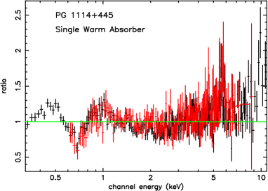
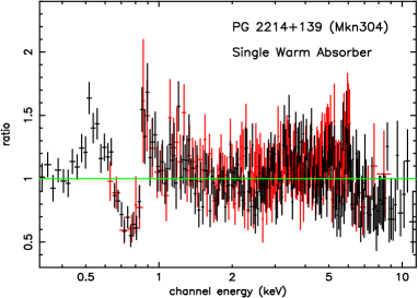
Figure 5: The ratios between the EPIC data (pn data in black, MOS in red) and a fit with single warm absorber model for 1114+445 (left) and 2214+139 (right): the large residuals below 1 keV strongly suggest the presence of a complex “multi-component” warm absorber. Note also the residuals around 5-6 keV which indicate Fe K$\alpha$ fluorescence emission (e.g. Paper II).

1115$+$080. XMM–Newton data of this BAL quasar have been also analyzed by Chartas et al. (2003). This study revealed an absorbed soft energy spectrum. Even though Chartas et al. (2003) suggested that the soft spectrum is best fitted by an ionized absorber, our study found that a neutral absorption model cannot be ruled out. Our analysis indicates that the best fit model for the observed spectrum consists of a power law modified by cold absorption and two absorption edges at $7.1^{+0.3}_{-0.4}$ keV and $9.5\pm 0.3$ keV (see Table 10 for further details). Taking into account Chartas et al. (2003) results, we have tried to explain the soft energy absorption by an ionized absorber using the ABSORI model in XSPEC. The value found for the ionization parameter ($\xi$) is extremely low and therefore the model does not differ from the neutral absorption one.

1226$+$023 (3C 273) The main feature in the pn spectrum of this well–known radio–loud QSO is the broad soft excess. A simple two-component model indeed fails to adequately describe its 0.3–12 keV emission (see Sect 3.2 and Fig. 2). Our best fit includes two blackbody components (with kT${}_{BB,1}\approx$ 0.1 and kT${}_{BB,2}\approx$ 0.24 keV, respectively) and a power law with a quite flat photon index ($\Gamma$ = 1.60$\pm$0.01). This result confirms the finding by Page et al. (2004a), based on the same XMM–Newton observation. We also detected the significant (at $>$ 99.9% confidence level) presence of an absorption edge at 7.4${}^{+0.1}_{-0.2}$ keV and with an optical depth of $\tau$ = 0.09${}^{+0.02}_{-0.03}$. Such an energy centroid suggests that the absorbing material is weakly ionized (Fe V–XV). The most likely origin for this edge feature is via reflection in optically thick matter as an origin in a line–of–sight plasma is not supported by the RGS data analysis results published in Page et al. (2004a), which did not report any absorption features apart from a OVII He$\alpha$ due to warm gas in the local intergalactic medium. Consequently, we also tried to fit the data with a model including a Compton reflection component (PEXRAV in XSPEC), yielding, however, no statistical improvement respect to the best fit model listed in Table 10. The upper limit for the covering factor of the material irradiated by the X–ray source is $R=\Omega/2\pi=$ 0.4. On the other hand, no Fe K$\alpha$ emission line (i.e. another hallmark of reprocessing in an accretion disk) was detected, and the upper limit on the equivalent width for a narrow line at 6.4 keV resulted to be 6 eV. Finally, Page et al. (2004a) reported the evidence for a weak broad Fe line using ten co-added EPIC observations which is, however, not detected in our data even when the absorption edge has been removed from the fitting model.

1404$+$226. This narrow line QSO was observed by ROSAT and ASCA. Ulrich et al. (1999) reported a very steep soft X-ray continuum, and evidence of complex ionized absorber. In particular, a peculiar absorption feature around 1 keV led these authors to claim for deviations from solar abundances in this source. Our results confirm the spectral complexity of 1404$+$226: we have found a best fit model consisting of a blackbody with kT = 0.144${}^{+0.002}_{-0.003}$ keV and a steep ($\Gamma$ = 2.34${}^{+0.35}_{-0.37}$) power law modified by ionized absorption. For the gas we derive a column density N_H $\approx$ 1.4 $\times$ 10²² cm^-2 and an ionization parameter $\xi$ = 44${}^{+123}_{-26}$ erg cm^-2 s^-1. No evidence of elemental abundances different from solar values have been found. Finally, no significant fluorescence iron emission line has been detected.

1411$+$442. This BAL QSO is X–ray faint ($F_{0.3-12}\approx$7 $\times$ 10^-13 erg cm^-2 s^-1). The 2–10 keV spectrum is extremely flat with a $\Gamma_{2-12}\approx$ 0.4 and a clear excess around 6 keV. The addition of a line with a narrow gaussian profile to parameterize the Fe K$\alpha$ emission feature produced a very significant (at 99.8% confidence level) improvement in the fit. The centroid ($E_{K\alpha}$ = 6.43${}^{+0.05}_{-0.13}$ keV) and narrowness of the line suggest a likely origin from a neutral material located far away from the innermost regions of the accretion disk.

The best fit model requires a power law with partial–covering (ZPCF in XSPEC) and a Raymond–Smith plasma component (this latter significant at $>$99.9% confidence level). For the absorbing gas we obtained a column density N_H $\approx$ 2.3 $\times$ 10²³ cm^-2 and a covering fraction of 96%. The plasma temperature and the photon index of the power law resulted to be kT =0.15$\pm$0.03 keV and $\Gamma$ = 2.3$\pm$0.2, respectively.

The limited statistics did not allow us to test more complex fitting models aimed, for instance, at checking the presence of a warm absorber in this source as observed in other AGNs with prominent absorption lines in the UV spectrum (e.g. Crenshaw et al. 2003; Monier et al. 2001; Piconcelli et al. 2004). This EPIC observation has been also analyzed by Brinkmann et al. (2004a) which reported results consistent with ours.

2214$+$139 (MKN 304). Our analysis matches well with previous results based on Einstein and ROSAT observations, which reported a very flat continuum for this source, and suggested the likely existence of heavy absorption. The XMM–Newton data reveal a complex spectrum, dominated by strong obscuration due to ionized gas (see Fig. 5). With a N_H $\approx$ 10²³ cm^-2, it is one of the ionized absorber with the highest column density seen so far by XMM–Newton and Chandra. A two–component warm gas provides an excellent description of this absorbing plasma. From the spectral analysis we derived $\xi^{T5}$ = 89.3${}^{+13.9}_{-12.0}$ erg cm^-2 s^-1 and $\xi^{T4}$ = 5.9${}^{+2.4}_{-0.9}$ erg cm^-2 s^-1 for the hot (i.e. with T = 1.5 $\times$ 10⁵ K) and the cold (i.e. with T = 3 $\times$ 10⁴ K) component, respectively. In addition to a narrow Fe K$\alpha$ emission line at $\sim$ 6.4 keV, another emission line feature was significantly detected at 0.57 keV, likely due to the helium–like oxygen triplet (maybe originating in the warm absorber itself). We also reported the presence of a weak soft excess component which can be interpreted as partial covering or scattered emission from the ionized outflowing plasma. For the complete and detailed presentation and discussion of these results see Piconcelli et al. (2004).

3.5 Fluxes and luminosities

Flux in the soft (0.5–2 keV) and hard (2–10 keV) energy band assuming the best fit model for each quasar as in Table 10 are listed in Table 11, together with the corresponding luminosities corrected for both the Galactic absorption and (if present) the additional intrinsic warm/neutral absorber column densities. The hard (soft) X–ray fluxes range from $\sim$ 0.1(0.1) to $\sim$ 80(45) $\times$ 10^-12 erg cm^-2 s^-1. With a 0.5–10 keV X–ray luminosity of $\sim$ 10⁴³ erg s^-1, 1001$+$054 is the faintest object in the sample. The most luminous quasar in the hard (soft) band is 1226$+$023 (1407$+$265) with a luminosity of $\sim$ 50 $\times$ 10⁴⁴ erg s^-1. In the two last columns of Table 11, the ratio between the strength of the soft excess and the high energy power law component in the 0.5–2 and 0.5–10 keV band are listed.

Table 11: Fluxes and absorption-corrected luminosities calculated assuming the best fit model. The last two columns list the ratio between the strength of the soft excess and the high energy power law component in the 0.5–2 and 0.5–10 keV band, respectively

PG Name	F${}_{0.5-2\,keV}$	F${}_{2-10\,keV}$	L${}_{0.5-2\,keV}$	L${}_{2-10\,keV}$	$R^{0.5-2}_{S/P}$	$R^{0.5-10}_{S/P}$
	(10-12 erg cm2 s-1)	(10-12 erg cm2 s-1)	(1044 erg s-1)	(1044 erg s-1)
0007$+$106	3.7	7.2	0.87	1.4	0.160	0.072
0050$+$124	9.15	8.44	1.39	0.78	0.360	0.212
0157$+$001	1.33	0.93	1.05	0.71	0.169	0.126
0804$+$761	11.6	11.12	3.43	2.86	0.489	0.238
0844$+$349	6.9	5.5	0.81	0.55	0.954	0.444
0947$+$396	1.79	1.87	2.55	2.26	0.814	0.336
0953$+$414	3.79	3.21	7.77	5.41	0.836	0.379
1001$+$054	0.03	0.12	0.10	0.13	$-$	$-$
1048$+$342	1.24	1.46	1.07	1.10	0.712	0.277
1100$+$772	2.48	3.83	8.97	11.19	0.650	0.318
1114$+$445	0.62	2.3	2.65	1.45	1.75	0.724
1115$+$080	0.23	0.36	42.1	65.3	$-$	$-$
1115$+$407	2.13	1.27	1.67	0.85	0.787	0.427
1116$+$215	5.2	3.3	5.0	3.1	0.473	0.258
1202$+$281	2.68	3.72	2.22	2.68	0.646	0.226
1206$+$459	0.14	0.24	8.55	14.9	$-$	$-$
1211$+$143	3.0	3.1	0.61	0.50	1.825	0.572
1216$+$069	1.08	1.38	4.69	4.8	0.948	0.351
1226$+$023	43.81	78.74	31.75	51.05	0.310	0.103
1244$+$026	5.87	2.53	0.36	0.14	0.470	0.297
1307$+$085	0.94	2.01	0.63	1.19	0.443	0.118
1309$+$355	0.45	0.73	0.46	0.67	0.175	0.077
1322$+$659	2.25	1.33	2.21	1.08	0.650	0.367
1352$+$183	2.30	2.00	1.85	1.36	1.121	0.464
1402$+$261	3.0	1.9	2.7	1.4	0.851	0.427
1404$+$226	0.51	0.10	2.31	2.87	0.423	0.246
1407$+$265	0.94	0.80	53.31	41.20	0.105	0.058
1411$+$442	0.09	0.46	0.35	0.25	0.061	0.062
1415$+$451	1.4	1.1	0.5	0.4	0.696	0.331
1427$+$480	1.2	1.1	2.0	1.6	0.634	0.284
1440$+$356	5.9	3.9	1.0	0.58	2.432	1.076
1444$+$407	0.9	0.6	2.6	1.3	3.009	1.420
1501$+$106	17.2	16.2	0.57	0.49	0.761	0.311
1512$+$370	1.56	1.97	8.51	8.84	2.050	0.859
1613$+$658	2.77	4.15	1.40	1.78	0.327	0.121
1626$+$554	3.04	3.08	1.57	1.46	0.708	0.354
1630$+$377	0.14	0.15	31.1	20.9	1.570	0.774
1634$+$706	1.0	1.16	141.6	127.9	0.591	0.335
2214$+$139	0.31	3.26	0.39	0.48	0.168	0.111
2302$+$029	0.24	0.27	25.9	16.2	0.649	0.336

Table 12: Spearman–rank correlations among spectral parameters of the soft excess tested models and X–ray parameters (luminosity and $\Gamma_{2-12}$). The displayed values are (r_s, $P_{s}$), where r_s is the rank correlation coefficient and $P_{s}$ is the significance probability. The significant (i.e. $>$ 95%) correlations are marked in boldface (see text for details).

		kTBB	kTDiskBB	kTBrem	$\Gamma_{Soft}$
L${}_{0.5-2\,keV}$		(0.46,97.9)	($-$0.26,82.4)	(0.41,96.8)	($-$0.15,52.1)
L${}_{2-10\,keV}$		(0.48,98.5)	($-$0.22,73.1)	(0.44,98.2)	($-$0.23,73.7)
$R_{S/P}^{0.5-2}$		(0.04,13.3)	($-$0.09,35.1)	($-$0.07,29.0)	(0.39,94.7)
$R_{S/P}^{0.5-10}$		(0.12,41.2)	($-$0.11,42.3)	($-$0.10,39.9)	(0.45,97.4)
$\Gamma_{2-12}$		(0.26,78.1)	($-$0.20,70.8)	($-$0.07,27.6)	(0.33,89.4)

3.6 Correlations among spectral parameters and luminosity

We performed Spearman–rank correlation tests. This test calculates how well a linear equation describes the relationship between two variables by means of the rank correlation coefficient (r_s) and the probability ($P_{s}$). Positive(negative) values of r_s indicates the two quantities are (anti–)correlated, while $P_{s}$ gives the significance level of such a correlation. In particular, we checked the type and strength of the relationship among the representative parameter of each model (i.e. kT_BB, kT_DiskBB, kT_Brem, $\Gamma_{Soft}$; see Sect. 3.2) and L${}_{0.5-2\,keV}$, L${}_{2-10\,keV}$, $R_{S/P}^{0.5-2}$ and $R_{S/P}^{0.5-10}$ and $\Gamma_{2-12}$ (see Table 11 and Table 3). The corresponding results are listed in Table 12.

This study reveals that none of the 20 pairs of parameters are significantly (i.e. $>$ 99%) correlated. Nevertheless, we found marginal hints of a non–trivial correlation for five of them, i.e. kT_BB–L${}_{0.5-2\,keV}$, kT_BB–L${}_{2-10\,keV}$, kT_Brem–L${}_{0.5-2\,keV}$, kT_Brem–L${}_{2-10\,keV}$ and $\Gamma_{Soft}$–$R_{S/P}^{0.5-10}$. Some of these correlations appear to be driven by the higher luminosity QSOs, $L_{2-10}$ $>$ 10⁴⁵ erg s^-1. For those relationships with $P_{s}>$ 95%, we also performed a linear regression fit to the data which, contrary to the Spearman–rank correlation test, takes also into account the uncertainties associated to the measurements. The values of $\chi^{2}$ obtained by each fit revealed that the probability that the two quantities are linearly correlated is lower than 50%.

3.7 Correlations with general source properties

Table 13: Spearman–rank correlations among X–ray observables and the radio-loudness parameter $R_{\rm L}$, the redshift, the FWHM of the H_β emission line, the black hole mass M_BH and the accretion rate $\dot{m}$ respect to the Eddington rate. The displayed values are (r_s, $P_{s}$), where r_s is the rank correlation coefficient and $P_{s}$ is the significance probability. The significant (i.e. $>$ 95%) correlations are marked in boldface (see text for details).

		L${}_{2-10\,keV}$	$R_{S/P}^{0.5-10}$	$\Gamma_{2-12}$	$\Gamma_{Soft}$
$R_{\rm L}$ (a)		(0.12,55.2)	($-$0.48,99.8)	($-$0.003,2.0)	($-$0.37,93.2)
$z$		(0.76,99.9)	(0.24,85.2)	(0.08,39.0)	($-$0.07,25.7)
FWHM(Hβ)(b)		(0.50,99.7)	($-$0.12,51.1)	($-$0.62,99.9)	($-$0.54,98.6)
MBH(c)		(0.67,99.9)	($-$0.03,13.1)	($-$0.52,99.8)	($-$0.16,51.2)
$\dot{m}$(d)		($-$0.39,97.5)	($-$0.05,19.0)	(0.41,97.9)	($-$0.09,30.1)

Data taken from: ^(a) Kellermann et al. (1994); ^(b) Boroson & Green (1992); ^(c) Gierlinski & Done (2004), P04 and Shields et al. (2003); ^(d) P04, Shields et al. (2003), and Woo & Urry (2002).

We also investigated by the Spearman–rank test the possible correlations among the most representative X-ray observables inferred by our analysis (i.e. L${}_{2-10\,keV}$, $R_{S/P}^{0.5-10}$, and $\Gamma_{2-12}$, $\Gamma_{Soft}$) and some QSO physical characteristics as the radio-loudness parameter $R_{\rm L}$, the redshift, the FWHM of the H_β emission line, the black hole mass M_BH and the accretion rate $\dot{m}$ relative to the Eddington limit (i.e. $\dot{m}$ = $\dot{M}$/$\dot{M}_{Edd}$). The results of the correlation analysis are presented in Table 13. We report significant and strong anticorrelations between the spectral indices $\Gamma_{2-12}$ and $\Gamma_{Soft}$ and the H_β FWHM confirming these well-known relationships found for both QSO–like (Reeves & Turner 2000; P04; Laor et al. 1997) and Seyfert–like AGNs (Brandt, Mathur & Elvis 1997). As already obtained for a smaller sample of PG QSOs by P04, the hard band slope also appears to anticorrelate with the black hole mass and to correlate with the fractional accretion rate $\dot{m}$. This latter, furthermore, has been found to be inversely linked with the L${}_{2-10\,keV}$ with a significance of $P_{s}$ = 97.5%, i.e. larger than in P04. PG QSOs with small M_BH tend to be less X–ray luminous. Laor (2000) pointed out that nearly all the PG RLQs with M_BH $>$ 10⁹ M_⊙ are radio-loud and this fact could be have represented a bias in our correlation analysis. The (anti-)correlations between ($\Gamma_{2-12}$)L${}_{2-10\,keV}$ and M_BH still holds when RLQs are excluded. An interesting discovery yielded by the present analysis is the very significant ($P_{s}$ $>$99%) anticorrelation between the radio-loudness $R_{\rm L}$ and $R_{S/P}^{0.5-10}$, i.e. the ratio between the strength of the soft excess and the high energy power law component in the 0.5–10 keV band. This finding seems to indicate that the soft excess emission in RLQs is less prominent than in RQQs. However, a larger number of objects with $R_{\rm L}$ $>$ 10 (i.e. radio-loud) is needed to confirm the robustness of this relationship. Finally, no correlation among the three X-ray observables and redshift was detected apart of the trivial case (L${}_{2-10\,keV}$, $z$) which is due to selection effects. Fig. 6 shows the plots corresponding to the very significant (i.e. at $>$99% confidence level) non-trivial correlations found in our analysis.

Figure 6: Significant (i.e. at $>$99% confidence level) correlations found among X–ray observables and QSO physical properties (See Table 13 and text for details).From top-left to bottom: (a) FWHM(H_β) versus L${}_{2-10\,keV}$; (b) M_BH versus L${}_{2-10\,keV}$ ; (c) FWHM(H_β) versus $\Gamma_{2-12}$; (d) $\Gamma_{2-12}$ versus M_BH; (e) $R_{S/P}^{0.5-10}$ versus $R_{\rm L}$.

4 Discussion

4.1 The Hard X–ray continuum

In Section 3.1 we presented the results for the power law fit in the high energy (2-12 keV) band for all the QSO. The $\chi^{2}$ analysis shows that the fits are acceptable, i.e. $\chi_{\nu}^{2}<1.2$, in all but four cases, i.e. 1411$+$442 ($\chi_{\nu}^{2}=1.66$); 1440$+$356 ($\chi_{\nu}^{2}=1.66$); 1630$+$377 ($\chi_{\nu}^{2}=1.70$); 2214$+$139 ($\chi_{\nu}^{2}=1.83$). Except for 1630$+$377, absorption was significantly detected in all these QSOs, being the most probable cause for the poor quality of the fit. In the case of 1630$+$377, the presence of an intense iron line could be responsible for the large $\chi_{\nu}^{2}$.

The mean value found for the index of the power law was $\Gamma_{2-12\,keV}=1.87^{+0.09}_{-0.10}$ and shows a significant spread, $\sigma=0.36^{+0.08}_{-0.06}$. The mean photon index is in good agreement with the results found from observations with previous satellites. Reeves & Turner (2000) and George et al. (2000) reported an average $\Gamma_{2-10\,keV}$ = 1.89$\pm$0.05 and $\Gamma_{2-10\,keV}$ = 1.97${}^{+0.08}_{-0.09}$ observing, respectively, 27 and 26 RQQs with ASCA (we compare $\Gamma_{2-12\,keV}$ with results from RQQ samples since RQQs represents $\sim$ 90% of our objects). A higher (but consistent with ours within the statistical uncertainties) value was derived from BeppoSAX data of 10 QSOs, i.e. $\Gamma_{2-10\,keV}=2.0\pm 0.3$ (Mineo et al. 2000). It has been observed in several studies (Zamorani et al. 1981; Reeves & Turner 2000) that RLQs have flatter spectral indices that the RQQs. Our results confirm this trend with these mean values for the photon indices: $\Gamma_{\rm{RLQ}}$ = 1.63${}^{+0.02}_{-0.01}$ and $\Gamma_{\rm{RQQ}}=1.89\pm 0.11$. The possible flatness of the spectral index for RLQs is consistent with a different process being responsible for the emission in the two type of QSO. While in RQQs the X-ray emission is thought to be associated to Compton up-scattering of soft photons originated in the accretion disk by hot electrons with a thermal distribution probably located in a corona above the accretion disk (Haardt & Maraschi 1993; Reeves & Turner 2000), in RLQs the effect of the relativistic jet could play an important role in the X-ray emission (Ghisellini et al. 1985; Reeves & Turner 2000). Even though our results favor the fact that the spectral index in RLQs is flatter than in RQQs, a study of a large sample of RLQs observed with ASCA (Sambruna et al. 1999) showed that comparing RLQs and RQQs which match in X–ray luminosity, there is no clear evidence of a difference in the spectral slope of these two types of QSOs.

We note that our mean $\Gamma_{soft}$ = 2.73${}^{+0.12}_{-0.11}$ (see Table 9) is similar to that found by Laor et al. (1997), i.e. $\Gamma_{soft}$ = 2.62$\pm$0.09. Therefore XMM–Newton EPIC results on the QSO overall spectral shape appear to be consistent with those from ROSAT PSPC and ASCA GIS/SIS observations.

Finally, a very significant ($P_{s}>$ 99%) (anti-) correlation between ($\Gamma_{2-12\,keV}$)L${}_{2-10\,keV}$ and the black hole mass was found (e.g. P04 and Sect. 3.7). Moreover, both these relationships still hold if only RQQs are considered. This points to the possibility that the black hole mass could play a major role in the definition of the hard X-ray properties in a QSO. Interestingly, a similar suggestion is reported by Laor (2000) who found a clear bimodality in the radio–loudness distribution as a function of the M_BH in the PG sample. These results can provide new insights on the investigations of the ultimate driver of the AGN activity.

4.2 The Soft excess

The systematic modeling of the 0.3–12 keV emission by different two–component continua presented in Sect. 3.2 allows us to infer useful insights on the physical nature of the soft excess.

It is worth to note the ubiquity of such a spectral component: we detected a low–energy X–ray turn–up in 37 out of 40 QSOs. Previous studies based on ASCA (George et al. 2000; Reeves & Turner 2000) and BeppoSAX (Mineo et al. 2000) QSO samples reported the detection of an excess of emission with respect of the high energy power law below 1–1.5 keV in $\sim$ 50–60% of the objects. However, as pointed out by these authors, it should be borne in mind the limited statistics (in the case of some BeppoSAX exposures) and the limited bandpass (0.6–10 keV in the case of ASCA) affecting these observations.

All the models applied to account for the soft excess component (i.e. blackbody, multicolor blackbody, bremsstrahlung and a power law) provided a statistically acceptable description of the broad–band X–ray spectrum for the majority of QSOs. In the following we discuss our results in the light of the physical scenario assumed in each tested model.

In first order approximation, the emission due to a standard optically–thick accretion disk can be modeled by a blackbody or a multicolor blackbody components. The $\chi^{2}_{\nu}$ values obtained by the application of these two models reveal that these parameterizations provide a fair representation of the EPIC QSO spectra (e.g. Tables 5 and 6). Nevertheless, the observed values of kT_BB and kT_MB $\sim$ 0.15 keV exceed the maximal temperature for an accretion disk (e.g. Frank, King & Raine 1992 for a review) which is kT${}_{Max}\sim$ 20–40 eV for a black hole mass of 10⁷–10⁸ M_⊙ accreting at the Eddington rate. Furthermore, kT_Max is an upper limit to the disk temperature since the accretion could be sub–Eddington and/or outer parts of the disk would likely be cooler. Hence, the mean values showed in Table 9 for the temperature of blackbody (kT_BB) and multicolor blackbody (kT_MB) argue that these models must be considered just as phenomenological and not as physically consistent models. Such an “optically–thick” scenario is even more critical in those quasars with double blackbody component as the best fit for the soft excess. In fact, they show a soft energy feature too broad to be fitted by a single temperature blackbody and, consequently, the second blackbody component usually has an unrealistic kT_BB $\;\buildrel>\over{\sim}\;$ 0.25 keV.

The soft X–ray emission of starburst regions (SBRs) is known to be dominated by the emission from a one– or multi–component hot diffuse plasma at temperatures in the range of kT$\sim$0.1-1 keV (Ptak et al. 1999; Read & Ponman 2001; Strickland & Stevens 2000). This thermal emission can be represented by a bremsstrahlung model. We obtained that this model is an appropriate fit ($\chi^{2}_{\nu}<1.2$) to the soft excess emission of an important fraction of the objects in the sample, (i. e. 28 out of 37 QSOs) and is the best fit model for 8 sources. The mean temperature for the bremsstrahlung model obtained for the 28 objects of our sample, kT${}_{BS}=0.38\pm 0.03$ keV, is compatible with typical values in SBRs. The diffuse gas associated to the soft X–ray emission of the SBRs have typically abundances in the range 0.05-0.3$Z$_⊙(Ptak et al. 1999; Read & Ponman 2001). However, the bremsstrahlung model does not include any emission lines and therefore it is not possible to measure the abundances of the diffuse gas and test if they are compatible with the typical ones measured in SBRs. In order to determine these abundances, we fitted the spectra of the eight sources for which the bremsstrahlung model is the best fit model for their soft excess emission with the MEKAL model (Mewe et al. 1986) leaving the abundances as a free parameter. The resulting values of the abundances were in all cases consistent with zero with upper limits in the range 0.011–0.15$Z$_⊙. Except for two objects, 1634$+$706 with $Z\leq 0.15Z$_⊙  and 2303$+$029 with $Z\leq 0.1Z$_⊙, the abundances are therefore lower than the typical values observed in SBRs. Moreover, in the soft band, the X–ray luminosities of SBRs vary in the range of $10^{38-41}$ erg s^-1 (Ptak et al. 1999; Read & Ponman 2001) while the luminosities associated to the optically thin soft X–ray component for these 8 QSOs are in all cases above $8\times 10^{43}$ erg s^-1, and, therefore, two orders of magnitude larger than the typical SBRs values even considering extreme cases as Ultra–Luminous Infrared Galaxies (Franceschini et al. 2003). Hence, on the basis of the abundances and luminosities inferred for our QSOs, it is very unlikely that the bremsstrahlung emission could be associated to powerful emission from a starburst region.

Even if (at the moment) quite speculative, another possible physical interpretation for the bremsstrahlung model is the emission from a transition layer between the accretion disk and the corona, as proposed by Nayakshin et al. (2000). These authors indeed suggested that in the case of sources with SED dominated by the UV thermal disk emission (as the present PG QSOs) bremsstrahlung emission from such a layer could significantly contribute to the soft X–ray emission in AGNs and, also, plasma temperature of $\sim$ 0.4 keV should be observed.

Alternatively, the bremsstrahlung model can be interpreted, in a similar way of the blackbody and multicolor blackbody models, as a purely mathematical parametrization of the QSO continuum (e.g. Fiore et al. 1995).

The power law is also, obviously, just a functional form to describe the true soft excess emission, without any underlying specific physical scenario. For six QSOs in the sample the power law model resulted the best fit. Notably, two QSOs (i.e. 0804$+$761 and 1440$+$356) show a slope of the high energy power law particularly flat ($\Gamma_{hard}$ = 1.3$\pm$0.7 and $\Gamma_{hard}$ = 1.2${}^{+0.4}_{-0.2}$, respectively, but note the large errors). Furthermore both $\Gamma_{hard}$ are very marginally (or not) consistent with the $\Gamma_{2-12}$ measured for these QSOs, suggesting so the presence of a hard tail instead of a soft excess. Such a hard X–ray feature could be also related to a strong reflection component (or/and a peculiar variability behavior) which cannot be constrained due to limited EPIC bandpass. However, such a scenario seems to be unlikely for these QSOs because of the lack of a strong iron line in their spectra (not detected in 1440$+$356 and with an EW$\sim$100 eV in 0804$+$76; see Paper II). Interestingly both these QSOs are classified as Narrow Line Quasar (Osterbrock & Pogge 1985), a class of objects which usually shows extreme flux variations, steep X–ray slopes and very strong soft excess extending up to $\sim$ 3 keV in some cases (e.g. O’Brien et al. 2001). This seems also the case for 1440$+$356 where such a spectral component dominates the broad band X–ray luminosity (e.g. Table 11).

Comptonization of thermal disk emission has been suggest as a likely physical origin of the soft excess in the X–ray spectra of Type 1 AGNs. The electron population responsible of the up-scattering is thought to have a temperature cooler (typically from 0.1 to few keVs) than the population producing the observed hard X–ray emission (approximatively a power law in the 2–10 keV band) with a k$T_{e}$ $\;\buildrel>\over{\sim}\;$ 80 keV (Perola et al. 2002). The exact location of such an electron population is still an open issue: a warm skin on the disk surface (Rozanska 1999), a transition between a cold and a hot disk (Magdziarz et al. 1998), or a single hybrid non–thermal/thermal plasma (Vaughan et al. 2002 and reference therein) are the most viable candidates. Interestingly, this soft X–ray component would contain the bulk of the source bolometric luminosity.

According to this scenario, recent works (P04; Gierliński & Done 2004) indeed modeled the soft X–ray excess of PG QSOs by a ‘cool’ Compton–scattering medium. This fit successfully reproduces the QSO spectral shape. However, the typical value found for the electron temperature is k$T_{e}$ $\sim$ few hundred eVs, with a very small range of variation through the broad distribution in luminosity and black hole mass within the sample. As pointed out by different authors (Brinkmann et al. 2004b; Page et al. 2004b; P04) the major problem with the Comptonization fit is the limited bandpass of XMM–Newton that does not allow to adequately constrain neither the blackbody emission from the disk nor the exponential cut–off at high energy. So a plausible explanation for the observed narrow range of k$T_{e}$ values is an observational bias due to the lack of sensitivity below 0.3 keV in the EPIC data. Furthermore, as pointed out by P04, the inferred values of k$T_{e}$ imply an extreme compactness of the Comptonizing region, i.e. 0.1 gravitational radii ($\sim$ 10¹² cm). This size is difficult to explain even in a scenario where the hard X–ray continuum is thought to be produced in discrete magnetic flares (instead of a extended corona) above the accretion disk (e.g. Merloni & Fabian 2002 for a review). Nevertheless, Comptonization seems the most realistic interpretation for the nature of the soft excess in QSOs. Unfortunately, the spectral capabilities of Chandra and XMM–Newton are not sufficient enough to disentangle the well–known degeneracy between the k$T_{e}$ and the optical depth of the scattering plasma (e.g. Vaughan et al. 2002; Brinkmann et al. 2004b). EUV to very hard X–rays (i.e. few hundred keV) broad band observations can give the key contribution to solve this issue.

Gierliński & Done (2004) suggested to interpret the soft excess in RQQs as an artifact of unmodeled relativistically smeared partially ionized absorption according to the fact that strong O and Fe absorption features at 0.7–0.9 keV can lead to an apparent upward curvature below these energies mimicking the presence of a true soft excess component. This scenario predicts a very steep ($\Gamma\gg$ 2) intrinsic continuum slope in the hard X–ray band (i.e. $>$ 10 keV) for RQQs. However, such large values of the intrinsic (i.e. corrected both by reflection and absorption) photon index have not been observed neither by BeppoSAX or Ginga observations (e.g. Mineo et al. 2000 and Lawson & Turner 1997, respectively). Nonetheless, even if not in such a dramatic way, broad “warm” absorption features due to atomic transitions could impact at a minor level on the estimate of the real slope of the primary continuum emission. More sensitive high–energy spectroscopic studies carried out in the next future with Astro-E2 or Constellation–X will be able to definitively test this hypothesis.

On the basis of RGS observations Branduardi–Raymond et al. (2001) proposed to explain the observed soft excess in the Seyfert galaxies MKN 766 and MCG–6-30-15 in terms of strong relativistically broadened recombination H–like emission lines of O, N and C. However, as pointed out by Pounds & Reeves (2002), all the objects for which this interpretation seems to be feasible show low X–ray luminosity (i.e. $L_{X}\sim$ 10⁴² erg s^-1) and their soft excess component emerges very sharply below $\sim$ 0.7 keV from the extrapolation of the 2–10 keV power law. On the contrary, all the soft excesses observed in PG QSOs turn up smoothly below $\sim$ 2 keV. So this soft X–ray broad emission lines scenario seems to fail for the sources (all with $L_{X}>$ 10⁴³ erg s^-1) in our sample.

Finally, the finding of an anticorrelation between $R_{L}$ and $R_{S/P}^{0.5-10}$ (see Table 13) seems to support the hypothesis that the soft excess in radio–loud QSOs is due to an X–ray emission component originating in the jets.

4.3 The intrinsic absorption

4.3.1 Cold absorber

In order to study the presence of a cold absorber in QSOs, we have added a neutral absorption component to the different models tested. The analysis reveals that the majority of the spectra does not require this component, and that the equivalent hydrogen column is negligible in comparison with the Galactic one. Only three sources, all of them RQQs, show the presence of a cold absorber, i.e. 0050$+$124, 1115$+$080 and 1411$+$442. The two former ones have columns of N_H $\leq 10^{21}$ cm^-2 likely associated to their host galaxies. The strongest absorption was found for 1411$+$442, N_H = 2.3$\pm$0.4 $\times$ 10²² cm^-2, although due the low statistic of the data it is not possible to confirm if this feature is originated by a cold absorption or is indeed related to a warm absorber. The rarity of intrinsic neutral absorption observed here is in agreement with previous studies of optically–selected QSOs (Laor et al. 1997; Mineo et al. 2000) and, in general, with the findings of recent wide–angle deep XMM–Newton surveys (e.g. Barcons et al. 2002; Piconcelli et al. 2003; Caccianiga et al. 2004) which reported a small fraction of broad line AGNs with a significant cold absorption component in excess to the Galactic value.

Therefore, we can conclude that for PG QSOs there is a good correlation between optical spectral type and X–ray absorption properties in agreement with the predictions of the AGN Unification Models.

4.3.2 Warm absorber

Warm (i.e. partially ionized) absorber in active galaxies are revealed by the presence of absorption edges in their soft X–ray spectra (Pan, Stewart & Pounds 1990). In particular, OVII (0.739 keV) and OVIII (0.871 keV) absorption edges were the typical signatures of such ionized gas detected in ROSAT and ASCA low–resolution observations. Notably, Reynolds (1997) found a warm absorber in $\approx$ 50% of the well studied Seyfert galaxies.

The study of this spectral component took a remarkable step forward exploiting the higher resolution ($R>$ 100) of the grating spectrometers on–board XMM–Newton and Chandra. H– and He–like absorption lines of cosmically abundant elements such as C, O, Ne, Mg and Si are the most numerous and strongest features observed in the soft X–ray spectra of bright Seyfert 1 galaxies. The presence between 0.73 and 0.77 keV of the unresolved transition array (UTA, e.g. Behar, Sako & Kahn 2001) of iron M–shell ions is also particularly common. The X–ray absorption lines are typically blueshifted by a few hundreds km/s and show complex profile due to a wealth of kinematic components. The ionized material is therefore in an outflow and it generally shows multiple ionization states (Kaastra et al. 2000; Collinge et al. 2001; Piconcelli et al. 2004).

On the contrary, the properties of the warm absorber in QSOs are poorly known so far. Nonetheless, it is widely accepted that the presence of ionized absorbing gas in such high luminosity AGNs is not as common as in Seyfert galaxies. Laor et al. (1997) indeed detected it in $\leq$ 5% of the optically–selected QSO population, and, on the basis of large ASCA sample, Reeves & Turner (2000) and George et al. (2000) both confirmed the rare occurrence in their spectra of opacity due to ionized gas along line of sight. Bearing in mind the limited statistics, George et al. (2000) did not find, however, significant differences in the physical parameters of the warm absorber (i.e. ionization state and column density) in low and high luminosity AGNs.

The scenario emerging by our analysis is completely different. In fact, we significantly detect absorption features due to ionized gas in the spectrum of 18 out 40 QSOs, i.e. the 45% of the sample. This fraction is similar to what found for Seyfert galaxies. The detection rate of warm absorber appears therefore to be independent from the X–ray luminosity. This finding confirms the recent result of P04 based on a smaller sample of 21 QSOs observed by XMM–Newton, and put it on a sounder statistical ground.

As reported in Sect. 3.4 most of these absorption features are observed in the range 0.7–0.8 keV: this fact suggests they are likely due to the He–like O edge and/or the blend of M–shell Fe lines (UTA). In the case of the edges found in the high–energy portion of the spectrum around 7 keV (as in 1115$+$080, 1211$+$143 and 1226$+$023), the energy of these features is still consistent with an origin in ”neutral” material (i.e. FeI–V). So an alternative explanation in terms of reflection from the optically thick accretion disk cannot be ruled out. The edge detected at $\sim$ 9 keV in 1115$+$08 would imply an ionization state higher than FeXXVI, so the possible origin of this feature in an ionized outflow (with a velocity of 0.34$c$ to account for the observed blueshift) as proposed by Chartas et al. (2003) seems to be the most reasonable.

Due to the strength of the absorption features in their spectra, for 4 objects (i.e. 1001$+$054, 1114$+$445, 1404$+$226 and 2214$+$139) we could apply the ABSORI model in the fit and, consequently, derive some physical parameters of the warm absorber in these sources (see Table 10). For 2214$+$139 and the BAL QSO 1001$+$054 the inferred column densities of the ionized gas are larger than 10²³ cm^-2, i.e. among the highest seen by XMM–Newton and Chandra so far. Even more interesting are the results we report for 1114$+$445 and 2214$+$139. Their XMM–Newton spectra indeed show for the first time the evidence for a multi-zone warm absorber in both QSOs.

These findings agree with the recent results obtained for Seyfert galaxies which claim for a multiphase outflowing plasma as origin of the warm absorber. Unfortunately, due to the EPIC spectral resolution, we cannot draw any conclusion on the ionization structure (i.e. discrete or continuous) of the ionized wind.

All the QSOs in our sample classified as “Soft X–ray Weak” QSOs (SXWQs) by Brandt, Laor & Wills (2000) (namely 1001$+$054, 1411$+$442 and 2214$+$139) have been found to be heavily absorbed. This finding supports the hypothesis that the observed soft X–ray “weakness” of SXWQs is likely due to the presence of absorbing matter along line of sight instead of an “intrinsic” weakness due to a different SED and/or emission/accretion mechanisms at work in SXWQs with respect to “normal” QSOs. Furthermore, all SXWQs analyzed here also show prominent absorption lines in the UV and in 2 out of 3 SXWQs the absorption occurs in an ionized gas. These facts support the idea of a possible physical connection between UV and X–ray absorbers (Crenshaw, Kramer & George 2003).

5 Conclusions

We have presented the results of the spectral analysis of 40 QSOs EPIC spectra observed by XMM–Newton. These objects represents $\sim$ 45% of the complete PG QSOs sample. The main findings of our study are:

• The hard X–ray continuum slope resulted $\Gamma=$ 1.89$\pm$0.11 and $\Gamma=$ 1.63${}^{+0.02}_{-0.01}$ for the radio–quiet and radio–loud QSOs in the sample, respectively. These values are consistent with previous X–ray observations of these objects and, in particular, we confirm a flatter slope in RLQs than RQQs. Such a difference could suggest the presence of an extra–continuum contribution from the self–synchrotron Compton jet emission (Zamorani et al. 1981).
  

• The soft excess is an ubiquitous feature of the low energy X–ray spectrum of the optically–selected QSOs. We systematically fitted the spectrum of each object with four different two–component models. None of the two-component models tested provides an satisfactory description for all the QSO spectra. This result suggests that the shape of the soft excess is not an universal QSO property. Spectral parameters inferred by these fits strongly indicate that all the applied models should be interpreted as phenomenological (and not physical) parameterizations of the observed spectral shape. Direct thermal emission from the accretion disk is ruled out on the basis of the very high temperature derived for this optically–thick component. Emission from a thermal plasma in a starburst is also ruled out because of the very large X–ray luminosities observed in our QSOs. A double power law model provides as well a good description of some QSO spectra and corresponds to a double Comptonization scenario for the X–ray emission. However, as also suggested by other authors (e.g. Gierliński & Done 2004, Brinkmann et al. 2004b) current X–ray observations cannot effectively constrain the physical parameters of the two plasma due to the lack of sensitivity in the EUV and at few hundred keVs where the emission peaks of the two component are expected.
  

• Significant evidence of cold absorption was detected in only three objects. Of them, two show column density (N_H $\sim$ 10²¹ cm^-2) consistent with the contribution from the host galaxy. For 1411$+$442 (with N_H $\sim$ 10²³ cm^-2), there are strong indications that the obscuration occurs in an ionized medium (Brinkmann et al. 2004a). Our result therefore agrees with the prediction of the AGN Unified Models (as well as recent observational results from wide–angle X–ray surveys) on the relationship between optical classification and X–ray absorption properties.
  

• About 50% of the QSOs show warm absorber features in their spectra. This finding is in contrast with previous studies based on ASCA or BeppoSAX data, where warm absorbers appeared to be rare. The fraction we observed is similar to that inferred for Seyfert 1 galaxies. The existence of ionized gas along the line of sight is independent on the X–ray luminosity. For two QSOs with the highest S/N ratio (i.e. 1114$+$445 and 2214$+$139) we also significantly detected a complex (two–phase) warm absorber (see Piconcelli et al. 2004).
  

• All the SXWQs in the sample show evidence of obscuration (occurring in an ionized medium in most of the cases). This finding suggests that their ‘weakness’ is just a matter of absorption instead of an unusual shape of the spectral energy distribution of such a class of QSOs.
  

• We performed correlation analysis between the spectral parameters of the soft excess tested models and the X–ray luminosities (Sect. 3.6) as well as between the hard X–ray observables (i.e. L${}_{2-10\,keV}$, $R_{S/P}^{0.5-10}$ and $\Gamma_{2-12}$, $\Gamma_{Soft}$) and some physical parameters (i.e. $R_{L}$, $z$, FWHM(H_β) and $\dot{m}$) (see Sect. 3.7). We confirmed the anticorrelations between both photon indices and FWHM(H_β) as reported in previous papers (P04, Reeves & Turner 2000). We also found that $\dot{m}$ is inversely correlated with the L${}_{2-10\,keV}$ and that the black hole mass (anti-)correlates with ($\Gamma_{2-12}$)$L_{2-10\,keV}$. Furthermore, we discovered a very significant anti-correlation between $R_{L}$ and $R_{S/P}^{0.5-10}$, i.e. the ratio between the strength of the soft excess and the high energy power law component in the 0.5–10 keV band.

The XMM–Newton view of optically–selected QSOs suggests that there are no significant changes in the spectral properties of these high luminosity AGNs once compared with the low luminosity broad line Seyfert galaxies. See also Paper II for the properties of the fluorescent iron K–shell emission lines in the same objects studied here.

- (1) Anders, E., & Grevesse, N., 1989, Geochim. Cosmochim. Acta, 53, 197
- (2) Arnaud, K.A., 1996, ASP Conf. Ser. Vol. 101, Astronomical Data Analyis and Systems, 17
- (3) Ashton, C.E., Page, M.J., Blustin, A. J., et al., 2004, MNRAS in press
- (4) Barcons, X., et al., 2002, A&A, 382, 522
- (5) Behar, E., Sako, M., & Kahn, S.M., 2001, ApJ, 563, 497
- (6) Bennett, C.L., et al., 2003, ApJS, 148, 1
- (7) Brandt, W. N., Mathur, S., Elvis, M., 1997, MNRAS, 285, 25
- (8) Brandt, W. N., Laor, A., & Wills, B. J., 2000, ApJ, 528, 637
- (9) Branduardi–Raymond, G., et al., 2001, A&A, 365, 140
- (10) Brinkmann, W., Papadakis, I. E., Ferrero, E., 2004a, A&A,414, 107
- (11) Brinkmann, W.,Arevalo, P.; Gliozzi, M.; Ferrero, E., 2004b, A&A, 415, 959
- (12) Cappi, M., Matsuoka, M., Comastri, A., Brinkmann, W., Elvis, M., Palumbo, G. G. C., Vignali, C., 1997, ApJ, 478, 492
- (13) Caccianiga, A., et al., 2004, A&A, 416, 901
- (14) Chartas, G., Brandt, W. N., & Gallagher, S. C., 2003, ApJ, 595, 85
- (15) Collinge, M.J., et al., 2001, ApJ, 557, 2
- (16) Comastri, A., Setti, G., Zamorani, G., Elvis, M., Wilkes, B. J., McDowell, J. C., Giommi, P., 1992, ApJ, 384, 62
- (17) Crenshaw, D.M., Kraemer, S.B., George, I.M., 2003, ARA&A, 41, 117
- (18) Dickey, J. M., & Lockman, F.J., 1990, ARA&A, 28, 215
- (19) Done, C., Mulchaey, J.S., Mushotzky, R.F., Arnaud, K.A., 1992, ApJ, 395, 275
- (20) Elvis, M., Lockman, F., & Wilkes, B.J., 1989, AJ, 97, 777
- (21) Fiore, F., et al., 1995, ApJ, 449, 75
- (22) Franceschini, A., et al., 2003, MNRAS, 343, 1181
- (23) Frank, J., King, A., & Raine, D., 1992, Accretion Power in Astrophysics, Cambridge University Press
- (24) Gallo, L. C., Boller, T., Brandt, W. N., Fabian, A. C., & Vaughan, S., 2004, A&A, 417, 29
- (25) George, I.M., Fabian , A.C., 1991, MNRAS, 249, 352
- (26) George, I.M., et al., 1997, ApJ, 491, 508
- (27) George, I. M., Turner, T. J., Yaqoob, T., et al., 2000, ApJ, 531, 52
- (28) Ghisellini, G., Maraschi, L., & Treves, A., 1985, A&A, 146, 204
- (29) Gierliński, M. & Done, C., 2004, MNRAS, 349, L7
- (30) Haardt, F. & Maraschi, L., 1991, ApJ, 380, 51
- (31) Kaastra, J.S., Mewe, R., Liedahl, D.A., Komossa, S., Brinkman, A.C., 2000, A&A, 354, 83
- (32) Kellermann, K. I., Sramek, R., Schmidt, M., Green, R. F., 1994, AJ, 108, 1163
- (33) Iwasawa, K. & Taniguchi, Y., 1993, ApJL, 413, L15
- (34) Jimenez-Bailon, E., Piconcelli, E., Guainazzi, M., et al., 2004, A&A, submitted (Paper II)
- (35) Laor, A., 2000, ApJL, 543, 111
- (36) Laor, A., Fiore, F., Elvis, M., Wilkes, B. J., & McDowell, J. C., 1997, ApJ, 477, 93
- (37) Lawson, A. J., & Turner, M.J.L., 1997, MNRAS, 288, 290
- (38) Lockman, F. J., & Savage, B. D., 1995, ApJS, 97, 1
- (39) Loiseau, N., 2003, XMM-Newton Science Analysis Users Guide v2.1
- (40) Maccacaro, T., Gioia, I. M., Wolter, A., Zamorani, G., & Stocke, J. T., 1988, ApJ, 326,680
- (41) Magdziarz, P., Blaes, O. M., Zdziarski, A. A., Johnson, W. N., Smith, D. A., 1998, MNRAS, 301, 179
- (42) Mathur, S., Wilkes, B.J., Elvis, M., 1998, ApJ, 503, L23
- (43) Merloni, A., & Fabian, A.C., 2002, Proceedings of the Symposium on ‘New Visions of the X-ray Universe in the XMM-Newton and Chandra Era’, ESA–ESTEC, (astro-ph/0201531)
- (44) Mewe, R., Lemen, J. R., & Van den Oord, G. H. J., 1986, A&AS, 65, 511
- (45) Mineo, T., et al., 2000, A&A, 359, 471
- (46) Monier, E.M., Mathur, S., Wilkes, B., Elvis, M., 2001, ApJ, 59, 675
- (47) Morrison, R., & McCammon, D., 1983, ApJ, 270, 119
- (48) Murphy, E. D., Lockman, F., Laor, A., Elvis, M., 1996, ApJS, 105, 369
- (49) Nandra, K., George, I. M., Mushotzky, R. F., Turner, T. J., & Yaqoob, T. 1997, ApJL, 488, L91
- (50) Nayakshin, S., Kazanas, D., & Kallman, T. R., 2000, ApJ, 537, 833
- (51) O’Brien, P.T., et al., 2001, MNRAS, 327, 37O
- (52) Osterbrock, D. E., Pogge, R.W., 1985, ApJ, 297, 166
- (53) Page, K. L., et al., 2004a, MNRAS, 349, 57
- (54) Page, K. L., Schartel N., Turner M. J. L., & O’Brien, P. T., 2004b, MNRAS, in press, (astro-ph/0404444)
- (55) Pan, H.C., Stewart, G.C., Pounds, K.A., 1990, MNRAS, 242, 177
- (56) Perola, G.C., Matt, G., Cappi, M., 2002, A&A, 389, 802
- (57) Piconcelli, E., Cappi, M., Bassani, L., Di Cocco, G., Dadina, M., 2003, A&A, 412, 689
- (58) Piconcelli, E., Jimenez-Bailon, E., Guainazzi, M., et al., 2004, MNRAS, 351, 161
- (59) Porquet, D., Reeves, J.N., O’Brien, P.T., Brinkmann, W., 2004, A&A, 422, 85 (P04)
- (60) Pounds, K.A., & Reeves, J.N., 2002, Proc. of “New Visions of the X-ray Universe in the XMM-Newton and Chandra Era”, (astro-ph/0201436)
- (61) Ptak, A., Serlemitsos, P., Yaqoob, T., & Mushotzky, R., 1999, ApJS, 120, 179
- (62) ead, A. M. & Ponman, T. J. 2001, MNRAS, 328, 127
- (63) Reeves, J. N., & Turner, M. J. L., 2000, MNRAS, 316, 234
- (64) Reynolds, C.S., 1997, MNRAS, 286, 513
- (65) Rozanska, A., 1999, MNRAS, 308, 751
- (66) Sambruna, R. M., Eracleous, M., & Mushotzky, R. F., 1999, ApJ, 526, 60
- (67) Schartel, N., Schmidt, M., Fink, H. H., Hasinger, G., & Truemper, J., 1997, A&A, 320, 696
- (68) Schartel, N., et al., 2004, A&A, submitted
- (69) Schmidt, M., & Green, R. F., 1983, ApJ, 269, 352
- (70) Shields, G. A., et al., 2003, ApJ, 583, 124
- (71) Stark, A. A., et al., 1992, ApJS, 79, 77
- (72) Strickland, D. K. & Stevens, I. R., 2000, MNRAS, 314, 511
- (73) Ulrich, M.H., Comastri, A., Komossa, S., Crane, P., 1999, A&A, 350, 816
- (74) Vaughan, S., et al., 2002, MNRAS, 337, 247
- (75) Woo, K. H., & Urry, C.M., 2002, ApJ, 579, 530
- (76) Zamorani, G., et al., 1981, ApJ, 245, 357