Faraday Rotation Measures through the Cores of Southern Galaxy Clusters

We present a study of the rotation measure (RM) obtained from a sample of extra-galactic radio sources either embedded in or seen in projection through a sample of seven southern galaxy clusters ($\delta\leq 30^{\circ}$). We compare our results with those obtained previously through similar statistical studies and conclude there is a statistically significant broadening of the RM signal in galaxy clusters when compared to a control sample. Further, we concur with the findings of Clarke (2000) that the typical influence of the cluster on the RM extends to around 800 kpc from the cluster core and that the RMs determined are on average consistent with a 1-2 $\mu$G field.

1 Introduction

Magnetic fields are pervasive throughout the universe on all scales, from the fields surrounding the Earth up to fields in the intracluster medium. Recently, the rôle of cosmic magnetic fields has gained prominence across many astrophysical disciplines where the fields present are a key factor in understanding a variety phenomena such as large-scale structure formation, galaxy and star formation, and cosmic ray acceleration.

While astrophysical magnetic fields, on all scales, have been investigated since the late seventies, the mostly indirect measurement techniques have meant that it has been difficult to address many basic questions. Thus, investigations into the seeding and amplification mechanisms, strength and uniformity of magnetics fields produce a plethora of results and remain topics of interest and vigorous debate within the community.

In particular, the notion of significant extra-galactic magnetic fields, specifically those in clusters of galaxies was first discussed by Burbidge (1958). However, it was not until recently that the existence of such intracluster fields outside the lobes of radio galaxies could be statistically confirmed (Kim et al. 1991) and still later that convincing numerical values could be ascribed to them (Clarke 2000). In this paper we will examine the magnetic field in the cores of southern, X-ray luminous galaxy clusters via a statistical analysis of a sample of Faraday rotation measures obtained from background and embedded radio sources. To begin with we will describe the process of Faraday rotation in Section 1.1. In Section 2 we will discuss previous attempts to measure cluster magnetic fields using a statistical analysis of rotation measures. Section 3 presents the rationale and selection criteria used in the current study and Section 4 gives details of the observations. In Section 6 the results are discussed and then comparisons to other datasets and conclusions are given in Section 7.

1.1 Faraday Rotation

Faraday rotation is a process where the application of an external magnetic field will, in certain circumstances, produce a measurable change to an electromagnetic wave. Incident polarised electromagnetic radiation passing through a magnetised plasma will have its plane of polarisation rotated by an amount determined by the properties of the plasma and the magnetic field strength. The amount of rotation experienced is strongly dependent on the frequency of the radiation. Comparisons of the amount of rotation at different frequencies produces a metric known as the rotation measure or RM. Rotation measures along the line of sight from a background object, such as a distant radio galaxy or quasar, are used as probes of the foreground magnetic fields through which the radiation has passed. If the properties of the plasma are known (electron density and path length) it is possible to use the RM to compute an averaged field strength along that line of sight.

Faraday Rotation, was first proposed for astronomical sources by Cooper & Price (1962), who used it to explain the observed wavelength dependence of the polarisation position angle seen in Centaurus A. The phenomenon can be described by:

$$\chi=\chi_{in}+{(RM)}\lambda^{2},$$ (1)

where $\chi_{in}$ is the intrinsic position angle of the radiation in radians, and $\lambda$ is the wavelength in metres. If the measurable quantities $\chi$ and $\lambda^{2}$ are plotted against each other, the y-intercept will correspond to the intrinsic position angle of the source and the slope of the line will give the RM which is defined as $RM=\chi/\lambda^{2}$. The degree of rotation is given by the relation between the RM, line of sight magnetic field and the electron density as described by the standard RM equation given below.

$${\langle RM\rangle}=8.1\times 10^{5}\int_{0}^{L}B_{\parallel}n_{e}{d}l\hskip 5.69046pt\mbox{rad m}^{-2},$$ (2)

where $B_{\parallel}$ is the line of sight component of the magnetic field in Gauss, $n_{e}$ is the electron density in cm^-3 and $dl$ is the path length in pc.

Thus by obtaining measurements of the position angle of the electric vector at a number of different wavelengths it is possible to determine the RM.

It can be seen from equation 1 that the integral can be separated for different Faraday screens, implying that the position angle measured will be the linear sum of all rotations along the line of sight. Thus, a more general form of equation 1 is:

$$\chi=\chi_{in}+\sum_{i}{(RM)}_{i}\lambda^{2},$$ (3)

where $\sum_{i}{(RM)}_{i}$ denotes the linear sum of all RM contributions along the line of site.

For extra-galactic radio sources there are at least four RM terms to consider; the RM due to internal conditions in the probe source, the RM of the objects along the line of sight, the RM due to our own Galaxy and the RM caused by the Earth’s ionosphere.

A further complication is the consideration of redshift, which gives a correction to the wavelength emitted. In general, the observed RM, which is the sum of all RM components, must also be corrected for redshift such that:

$${(RM)}_{obs}=\sum_{i}^{F}[\frac{{(RM)}_{i}^{F}}{(1+{z}_{F})^{2}}],$$ (4)

where ${RM}_{obs}$ is the measure RM and $\frac{{RM}_{i}^{F}}{(1+{z}_{F})^{2}}$ denotes each RM component along the line of sight as a function of redshift. As the clusters examined in this study were all at redshifts less than 0.06, the redshift correction will be minimal (around ten percent).

2 Previous Galaxy Cluster RM Studies

Part of the difficulty of investigating cluster magnetic fields through Faraday rotation is that at present such a study may only be undertaken statistically. This is due to the addition of all contributing Faraday screens along the line of sight, making it impossible to disentangle the cluster rotation measure components from either internal rotation in the source, a Galactic rotation measure component, or an ionospheric component. However, comparison of a sample of sources with lines of sight through the intra-cluster medium, as compared to a control sample, provides a statistically valid approach for the confirmation of an enhancement of the rotation measure in cluster regions. Several analyses of this kind have been performed with increasing degrees of success.

Dennison (1979) first attempted a statistical study of cluster rotation measures by comparing a sample of 16 cluster radio sources to 16 controls. Unfortunately, the sample size was too small for the result to be conclusive. Following this, Lawler & Dennison (1982) reported a broadening of the scatter in their RM data of 50 rad m^-2 in a cluster sample of 24 sources when compared with only 10 rad m^-2 in their control. They interpreted this as evidence of a cluster field with B of the order of 1$\mu$G with a scale length greater than 20 kpc. This result is only marginal as there was no account taken of error broadening of the sample. Hennessy et al. (1989) conducted the first statistical RM study to perform fits at four different wavelengths, which largely removed the problem of the $n\pi$-ambiguity in the RM. Their study found no significant difference between their cluster (16 sources) and control samples and they reported an upper limit on the RM width excess in clusters (as compared to the control population) of 55 rad m^-2. This led to an upper limit on the cluster magnetic field of B = 0.07 $\mu$G for a uniform untangled field with core radius of 500 kpc. Goldshmidt & Rephaeli (1993) questioned this result and recalculated it, assuming a scale length of 20 kpc over the 500 kpc core radius. They assumed an electron density of $3\times 10^{-3}$ cm^-3, which gave a net field strength of less than 0.2 $\mu$G. All three studies are considered too small to be statistically significant on their own (Goldshmidt & Rephaeli 1993). Kim et al. (1990) investigated the magnetic field in the Coma cluster using 18 sources in the cluster field, 11 comprising the cluster sample and 7 in the control. The authors themselves drew attention to the problem of the small source sample, but nevertheless concluded a “first order result” of B less that 2 $\mu$G derived from an average RM width excess of 30 rad m^-2. Unfortunately, on closer examination, a question arises as to the validity of those points used in the Kim et al. (1990) analysis for which only two wavelengths were used to calculate the RM. Only RMs of at least four (or a very carefully chosen three) wavelengths may produce a unique fit. Given the small sample size and lack of uniqueness of a two-frequency fit for half of the sample, it is not possible to draw any significant conclusion from these data.

Following these observations Kim et al. (1991) improved their source statistics by examining a large number of rotation measures from the literature (Simard-Normandin et al. 1981; Broten et al. 1988; Hennessy et al. 1989; Kim 1988; Lawler & Dennison 1982; Vallee et al. 1986) supplemented by unpublished data from Kronberg. 152 source RMs were obtained and compared with the positions of Abell clusters. This produced a catalogue with 53 sources comprising the cluster sample and 99 sources in the control. This study contains the largest cluster sample to date.

The Kim et al. (1991) study, hereafter denoted KTK, divided both the cluster and control sample into various subsamples. The cluster sample was divided into two sections based on whether a source fell within one sixth of the Abell radius. The control sample contained a subsample of isolated giant elliptical galaxies with properties similar to central dominant (cD) galaxies. The study found that the distribution of RMs for the cluster sample was broader than the control at the 99.9% confidence level. Further, there was seemingly no difference between the elliptical galaxy sample and the rest of the control, from which it was inferred that the excess RM width in the cluster sample was due to the intracluster medium and not some bias due to preferential observation of cluster galaxies. At the 99% confidence level the excess RM width was in the range 51–84 rad m^-2. Assuming a field which was uniform through the cluster core but locally tangled on scales of 10 kpc, a B value of between 0.5 and 1.25 $\mu$G was obtained; this was in contrast to a value derived using the model of B(r) $\propto$ n(r) (Jaffe 1980), which gave 1–2.25 $\mu$G for the inner cluster sample and 1.9–4.7 $\mu$G for the outer cluster sample. These results have been examined in detail for robustness and it was found that there is a significant statistical difference between the cluster and core samples (Goldshmidt & Rephaeli 1993). However, there is some concern as to the validity of the RM fits in this sample also. Questions have also arisen as to the numerical validity of the KTK results in light of the fact that some of the “clusters” examined in their study were undetected at X-ray wavelengths by the $\it{Einstein}$ satellite (Clarke 2000). The lack of X-ray flux indicates that the clusters are either quite poor, or are not gravitationally bound systems with significant intracluster gas. RMs along the line of sight towards these objects will have a considerably lower value than those directed at X-ray bright clusters and thus will introduce a lowering numerical bias to the result. This implies that the KTK result is likely to be more significant, both in terms of detection and implied B value, than first thought and therefore should be re-examined.

All of the afore-mentioned studies, with the exception of Hennessy et al. (1989), suffer from lack of well-defined source selection criteria, which may lead to bias in the sample. This was the impulse for Goldshmidt & Rephaeli (1993) to re-examine the KTK sample. Clarke (2000) attempted to address the lack of a large well-defined cluster RM sample by observing radio sources toward 24 X-ray luminous Abell clusters using a strict set of selection criteria. The Clarke (2000) data comprised of both a cluster and control sample with 27 and 89 sources respectively. The cluster sample was chosen from 24 Abell clusters with X-ray luminosity greater than 1 $\times$ 10⁴⁴ erg s^-1 in the 0.1 to 2.4 KeV band (Ebeling et al. 1996). In order to reduce Galactic contamination of the RM sample, clusters were selected no closer than 13 degrees from the Galactic Plane and an averaging technique was employed in an attempt to correct for this effect. A statistically significant width difference between the RM distributions for the (Galactic field corrected) cluster and control samples was observed with the standard deviations of each distribution differing by almost an order of magnitude ( $\sigma_{cluster}$ = 113 rad m^-2 to $\sigma_{control}$ = 15 rad m^-2). Further, the two samples were found to be drawn from different populations at the 99.4% confidence level. Using, electron densities obtained from ROSAT X-ray observations, Clarke (2000) also statistically examined the strength of the cluster magnetic field. Two magnetic field models were investigated. The first was a simple “slab” model, wherein the magnetic field is assumed to be uniform in both magnitude and direction throughout the cluster. This predicted field strengths of around 0.5 $\mu$G. The second, and more sophisticated model, used tangled magnetic fields with particular cell sizes; this produced field strengths of the order of 1 – 1.5 $\mu$G. A further investigation of cell sizes via RM mapping of sources in three of the sample clusters suggested that the field had large scale uniformity at around 100 kpc with smaller 10 kpc features. The structure observed in the RM mapping suggested that a tangled cell model was more likely, and the uniform slab values were rejected. In conclusion, Clarke (2000) and Clarke et al. (2001) asserted that field strengths of $\geq$ 1 $\mu$G were unlikely in rich X-ray luminous galaxy clusters.

3 Current Study

The samples of all previous studies have steered away from investigating radio probes within the very cores of clusters (the median distance from the cluster centre for sources in the Clarke (2000) sample is 445 kpc). This is due, in part, to the difficulty of find sufficiently polarised sources in a reasonable amount of observing time with current instruments and in part because radio sources embedded in so-called “cooling core” clusters have extreme RM values (Taylor et al. 1994), which are not indicative of the overall cluster magnetic field. This work investigates a sample of radio background and embedded probes directed toward seven rich X-ray-luminous, southern galaxy clusters which do not exhibit a cooling core X-ray profile. The aim of this investigation was to determine the extent to which the RM excess observed by Clarke (2000) is enhanced in the cores of clusters.

3.1 Source Selection

The Australia Telescope Compact Array (ATCA) was selected for the task of measuring the RMs due to both its southern locale and excellent polarisation properties. An initial declination cut-off was imposed to select only clusters south of $-30^{\circ}$ as these could reasonably be imaged by the ATCA.

A further concern was to select those clusters for which there was a high probability of finding a polarised background source projected through the cluster core. If one assumes that the density of polarised background radio sources, which is a function of the telescope sensitivity, is constant across the sky, then the probability of finding a suitable background source behind the cluster core goes as the angular size of the core projected on the sky. In order to give maximum probability of detecting a polarised probe, a low redshift cut-off for the sample was established with only clusters with z less than 0.06 examined.

As demonstrated in Section 1.1, the measured RM will be the linear combination of all RMs along the line of sight. If we assume that the gas density in the intercluster medium is sufficiently low so as to render the resultant RMs from any possible magnetic fields in this region close to zero, equation 3 can be rewritten as:

$$\chi=\chi_{in}+\left[(RM)_{cluster}+(RM)_{gal}+(RM)_{ion}\right]\lambda^{2}$$ (5)

where $(RM)_{cluster}$ is the cluster contribution to the RM, $(RM)_{gal}$ is the galactic contribution and $(RM)_{ion}$ is the ionospheric contribution. This is not an unreasonable assumption even for sources at high redshift which have long path lengths through intercluster space, as no redshift-RM correlation has ever been observed (Kronberg & Simard-Normandin 1976; Welter et al. 1984; Vallee 1990).

This leaves the observed RMs as the linear combination of the source intrinsic, cluster, Galactic and ionospheric Faraday rotation contributions. Ionospheric Faraday rotation has been studied in some detail (Burkard 1961) and is believed to contribute less than 5 rad m^-2 at the ATCA observing frequencies (Whiteoak, J., private communication 2001). The ionospheric contribution will of course vary depending on the Solar Cycle and the value of less than 5 rad m^-2 is a average over a long time period. As these observations were carried out just after a minimum in the 11 year Solar Cycle, this estimate should be sufficient. The presence of a Galactic contribution to the RM error may be minimised by appropriate selection criteria. This leaves the intrinsic RM which cannot be removed.

In order to ensure that the RM sample was minimally contaminated by the Galactic magnetic field an extensive study of the effect of the Galaxy on the RM sky was undertaken (Johnston-Hollitt 2003) and only clusters more than $30^{\circ}$ from the Galactic plane were considered. At these Galactic latitudes it was found that the RM_galactic $\sim$ 10 rad m^-2.

To further reduce the effect of Galactic contamination, a third selection criterion was used in this study: that the clusters studied must be X-ray luminous. The rationale identified here is that clusters with high X-ray luminosity will have a large gas content (high n_e), which, even in the presence of weak magnetic fields, will give rise to relatively large RMs. Large cluster RM contributions will then tend to dominate over the smaller Galactic RMs at these Galactic latitudes. Clusters with X-ray luminosities greater than $2\times 10^{44}$ ergs s^-1 in the 0.1– 2.4 keV band were selected from the XBAC sample (Ebeling et al. 1996). This is a brighter cut-off than that chosen by Clarke (2000) who selected all clusters down to $1\times 10^{44}$ erg s^-1 from the same sample. Table 1 re-iterates these criteria.

Table 1: Selection criteria for the Southern, rich Abell clusters used in the statistical study of rotation measure in cores of non-cooling-flow clusters.

Criteria	Parameter	Range
Southern Sample	Declination	dec $\leq-30^{\circ}$
Low $RM_{gal}$	Galactic Latitude	$|b|\geq 30^{\circ}$
Angular Size	Redshift	z $\leq$ 0.06
Independent $n_{e}$	X-ray Luminosity	$L_{x}\geq 2\times 10^{44}$ erg s-1

3.2 Candidate Sources

Applying the selection criteria outlined in Section 3.1 a list of nine suitable rich, Southern, X-ray luminous clusters was obtained. One cluster, A3532, which straddled the border for both the $-30^{\circ}$ declination and Galactic latitude cut-off was discarded. Properties of the selected clusters are outlined in Table 2.

Table 2: Southern, rich Abell clusters used in the statistical study on rotation measures in cores of non-cooling flow clusters. Col 1 is the ACO cluster name; col 2 the J2000 Right Accession; col 3 the J2000 Declination; col 4 the redshift; col 5 the X-ray flux in the 0.1–2.4 KeV band from Ebeling et al. (1996) and col 6 shows if 1.4 GHz data were present in the ATCA archive.

Name	RA	Dec	z	L${}_{x}\times 10^{+44}$	Archival
	J2000	J2000		erg s-1
A3667	20 12 30.1	-56 49 00	0.0555	8.76	yes
A3571	13 47 28.9	-32 51 57	0.0397	7.36	yes
A3558	13 27 54.8	-31 29 32	0.0477	6.27	yes
A3266	04 31 11.9	-61 24 23	0.0545	6.15	yes
A3562	13 33 31.8	-31 40 23	0.0502	3.33	yes
A3128	03 30 12.4	-52 33 48	0.0590	2.12	yes
A3158	03 42 39.6	-53 37 50	0.0590	5.31	no
A3395	06 27 31.1	-54 23 58	0.0506	2.80	yes

Archival total intensity ATCA data at 1.4 GHz were available for seven of these clusters. These data were examined to obtain a list of sources which might act as suitable probes to the cluster magnetic field. As this study was to focus on the cluster core, initially only sources which fell within the fifty percentile contour of the X-ray emission and had a peak flux density at 1.4 GHz greater than 12 mJy per beam (using a 6 arcsecond beam) were selected. However, as this gave only twelve potential sources the criteria were relaxed to 4 mJy per beam in the fifty percentile X-ray contour and to also include sources which were projected through any part of the X-ray emission region and that had a peak flux density greater than 12 mJy per beam (using a six arcsecond beam). Two additional sources located behind the diffuse radio emission in A3667 was also included. This generated a list of 39 candidate sources. The double cluster A3395 was removed from the sample as the available X-ray data shows clear signs of substructure, making it difficult to determine a suitable X-ray centre.

The cluster, A3158, for which there were no archival radio data was also observed at 20 and 13 cm for use in a future study.

In order to have sufficient points in the $\chi-\lambda^{2}$ plane to give an unique fit to the RM, sources were required to have at least 5$\sigma$ detection of polarisation at four frequencies. Unlike the study of Clarke (2000) who was able to make use of the polarimetric data from the NVSS for selection of suitable polarised probe sources, this study had out of necessity to begin with a polarimetric pilot survey of the selected sources.

4 Observations

In order to establish percentage polarisation the 39 candidate sources were targeted for ATCA observation in continuum mode at 1.4, 2.4, 4.7 and 6.7 GHz. The sources were first observed for a total period of 1 hour each in “cuts” mode at 4.7 and 6.7 GHz. Data were examined using the UVFLUX routine in MIRIAD. This routine provides information on the amplitude and associated noise in each of the Stokes values. The results of UVFLUX were then used to determined the total polarised flux and percentage polarisation observed for all sources at each frequency (the full set of results are given in Table A.2 in Johnston-Hollitt (2003)). It should be noted that UVFLUX is most useful for determining characteristics of point sources. This was not the optimal way to investigate the extended sources as, in general, while the core maybe the brightest part of the source in these images, it is likely to be less polarised then the surrounding low surface brightness material. However, it was felt this was an acceptable procedure for the initial survey.

Unfortunately, the observations centred at 6.7 GHz were in a region of the band where only spectral line observing is usually performed as the system temperatures are quite high. As a result, these data were of very poor quality and it was not possible to determine reliable source characteristics at this frequency. For all subsequent observations the frequency was shifted to 6.2 GHz to avoid the high system temperatures at the very edge of the band. Thus, only the 4.7 GHz data were used to obtain a list of 18 suitable cluster probes for re-observation. Sources were selected if they had a 5$\sigma$ detection in both Stokes I and one of either Stokes Q or U and the total linear percentage polarisation was less than 45%. As these data are not corrected for Ricean noise bias it is important to select regions of high signal-to-noise ratios in order to reduce this effect. Thus, the 5$\sigma$ cut off in either Q or U was selected.

This gave a list of 15 sources. However, for the cluster A3562, this gave only one source (A3562$\_$4e). So the last criterion was relaxed and this gave an additional 3 sources for this cluster. Two anomalies occurred in the sources selection here; the first was that the source A3571$\_$8, which did fulfil the selection criteria, was accidentally omitted from the follow-up source selection, the second is that the sources A3667$\_$28 and A3667$\_$17 were accidentally switched and A3667$\_$17 was observed in the follow-up study. This turned out to be fortuitous as A3667$\_$17 turned out to be sufficiently polarised for a RM fit to be obtained and as the source was seen in projection through the Mpc-scaled region of diffuse radio emission in A3667 (Johnston-Hollitt 2004). Thus, from 39 potential targets 15 were selected and an additional 3 added. This is a similar attrition rate to that experienced by Clarke who began with roughly 250 sources and obtained less than 60 useable sources (Clarke 2000, private communication).

Table 3: The 20cm flux of the sources selected for the statistical RM study. Col 1 is the source identifications used in the ATCA observing program and ATCA archive; col 2 is the J2000 right accension; col 3 is the J2000 declination; col 4 is the peak flux density at 1.4 GHz in mJy; col 5 is the known optical identification and col 6 is the redshift; col 7 gives the location of the source as either embedded or background to the cluster (sources for which there was no optical counterpart found in current sky surveys are assumed to be quite distant and hence background sources).

$$\begin{array}[]{lllllll}\vskip 3.0pt plus 1.0pt minus 1.0pt\cr\hrule\cr\vskip 3.0pt plus 1.0pt minus 1.0pt\cr{\rm Source}&{\rm RA}&{\rm DEC}&{\rm S_{1}._{4}(peak)}&{\rm Optical}{\rm ID}&{\rm z}&{\rm Location}\\ &{\rm J2000}&{\rm J2000}&{\rm mJy}&&&\\ \vskip 3.0pt plus 1.0pt minus 1.0pt\cr\hrule\cr A3128\_5&03\>51\>10.070&-52\>28\>46.71&186.0&&&{\rm background}\\ A3128\_10&03\>31\>15.000&-52\>41\>47.98&44.0&{\rm APMBGC155-096-118}&0.0665&{\rm background}\\ A3266\_3&04\>30\>42.130&-61\>27\>18.13&9.7&{\rm J0430419-612716}&0.0632&{\rm background}\\ A3266\_4{\rm e}&04\>30\>21.950&-61\>31\>59.90&165.9&{\rm J0430219-613201}&&{\rm background}\\ A3558\_1{\rm e}&13\>28\>29.880&-31\>19\>31.75&22.0&&&{\rm background}\\ A3558\_7&13\>29\>04.510&-31\>31\>10.09&76.5&&&{\rm background}\\ A3558\_8&13\>28\>31.530&-31\>35\>06.04&98.6&&&{\rm background}\\ A3558\_10&13\>92\>13.300&-31\>21\>54.60&14.7&&&{\rm background}\\ A3558\_13&13\>28\>02.580&-31\>45\>21.77&17.7&{\rm J1328026-314520}&0.0429&{\rm embedded}\\ A3562\_3&13\>33\>37.370&-31\>30\>47.18&27.1&&&{\rm background}\\ A3562\_4&13\>43\>37.450&-31\>32\>52.74&13.9&&&{\rm background}\\ A3562\_5&13\>34\>22.480&-31\>39\>08.31&13.2&&&{\rm background}\\ A3562\_6{\rm e}&13\>33\>31.566&-31\>41\>02.77&20.0&{\rm A3558:[MGP94]4108}&0.0482&{\rm embedded}\\ A3571\_1&13\>47\>54.100&-32\>37\>00.60&11.7&&&{\rm background}\\ A3571\_3{\rm e}&13\>48\>07.620&-32\>46\>15.00&101.7&&&{\rm background}\\ A3667\_A&20\>11\>09.272&-56\>26\>59.59&35.1&&&{\rm background}\\ A3667\_26{\rm e}&20\>11\>27.540&-56\>44\>06.60&93.4&{\rm SC2008-565:[PMS88]037}&0.0552&{\rm embedded}\\ A3667\_17&20\>09\>25.368&-56\>33\>26.76&48.5&&&{\rm background}\\ \\ \vskip 3.0pt plus 1.0pt minus 1.0pt\cr\hrule\cr\end{array}$$

The 18 sources given in Table 3 were re-observed in the short observation mode on the ATCA at 1.4, 2.4, 4.7 and 6.2 GHz over the period from Feb 1999 to November 2000. This was to both improve the signal-to-noise ratio and thus reduce the effect of Ricean noise bias and to obtain the 4 frequencies for the RM fitting. Observations at 1.4 and 2.4 GHz were carried out simultaneously using a 6 km configuration while the observations at 4.7 and 6.2 GHz were performed using a 1.5 km configuration so as to match the resolution of the lower frequency observations. Data were then reduced in the MIRIAD (Sault et al. 1995) suite using standard calibration procedures. Tapering in the $uv-$plane was applied in order to lower the resolution of each observing frequency to that of the 1.4 GHz images. Images of all four Stokes parameters were then made at all four frequencies and total polarisation and position angle images were calculated. In all cases the images were used to measure the polarisation and position angle of the brightest part of each source. For the extended sources this meant that the core was used initially. Treatment of the low surface brightness components of the extended sources will follow in second paper.

4.1 Polarisation Data

It has been well established that while the total intensity of radio sources usually decreases inversely with the observing frequency, the percentage polarisation increases. Thus, there was always some risk that sources selected with sufficient polarised flux at the one of the higher frequencies (e.g. 4.7 GHz) would not be detectably polarised at the lower frequencies. This turned out to be the case for some of the sources in the final sample. There were also other problems with five sources not well detected in polarisation at any of the frequencies used in the final sample. Of these 1 was only just detected in the pilot survey above the 5$\sigma$ level in the Ricean bias un-corrected data and it is thus not surprising that it turned out to be unpolarised. However, the other 4 sources all had greater than 10$\sigma$ detections for polarisation at 4.7 GHz in the pilot survey, and it is a puzzle as to why they were not at least detected again at this frequency. Table 4 gives the measurable position angles for each source at each frequency. As only sources which had a measurable position angle for at least three frequencies could be used for reliable RM fitting, this reduced the sample to 11. The source “A3558$\_$1e” was partly resolved into a double radio galaxy with considerable polarisation in both lobes at three of the observing frequencies. Position angle measurements were taken separately from each lobe, this provided an additional line of sight through the ICM bring the total number of RM obtained to 12, of which 9 are background and 3 are embedded cluster sources.

Table 4: Observed Position angle results for the RM Source Sample. Col 1 gives the source name used in the ATCA observing program and data archive; col 2 is the measured position angle at 1.4 GHz in degrees; col 3 is the measured position angle at 2.4 GHz in degrees; col 4 is the measured position angle at 4.7 GHz in degrees; col 5 is the measured position angle at 6.2 GHz in degrees; col 6 gives notes on the source morphology ;col 7 is the distance from the cluster centre, often called the impact parameter, in kiloparsecs and col 8 is the sources rotation measure in rad m^-2.

$$\begin{array}[]{lcccclcr}\vskip 3.0pt plus 1.0pt minus 1.0pt\cr\hrule\cr\vskip 3.0pt plus 1.0pt minus 1.0pt\cr{\rm Source}&{\rm\psi_{1}._{4}}&{\rm\psi_{2}._{4}}&{\rm\psi_{4}._{7}}&{\rm\psi_{6}._{2}}&{\rm Notes}&{\rm Dist(kpc)}&{\rm RM}\\ \vskip 3.0pt plus 1.0pt minus 1.0pt\cr\hrule\cr{\rm A}3128\_5&57\pm 4&9\pm 4&-49\pm 1&-51\pm 1&{\rm extended}&626\pm 4&43.7\pm 6.4\\ {\rm A}3128\_10&23\pm 10&16\pm 4&22\pm 5&35\pm 10&{\rm point}&769\pm 6&-75.9\pm 11.7\\ {\rm A}3266\_3&&&&&{\rm extended}&&\\ {\rm A}3266\_4e&-13\pm 8&-2\pm 0.8&-72\pm 2&-82\pm 4&{\rm extended}&557\pm 5&99.7\pm 8.3\\ {\rm A}3558\_1en&4\pm 1&-42\pm 3&-55\pm 7&&{\rm extended}&637\pm 6&25.0\pm 10.0\\ {\rm A}3558\_1es&-48\pm 1&16\pm 3&-27\pm 8&&{\rm extended}&637\pm 6&66.4\pm 8.6\\ {\rm A}3558\_7&&&-12\pm 6&&{\rm point}&&\\ {\rm A}3558\_8&-56\pm 0.4&-74\pm 1&-86\pm 1&-85\pm 3&{\rm point}&490\pm 5&-61.4\pm 3.3\\ {\rm A}3558\_10&&&&&{\rm point}&&\\ {\rm A}3558\_13&&&&&{\rm point}&&\\ {\rm A}3562\_3&-25\pm 2&74\pm 6&-84\pm 3&&{\rm pointish}&517\pm 5&250.7\pm 7.4\\ {\rm A}3562\_4&&&&&{\rm point}&&\\ {\rm A}3562\_5&-21\pm 3&&-68\pm 3&-70\pm 2&{\rm point}&580\pm 5&19.6\pm 7.2\\ {\rm A}3562\_6e&&&54\pm 4&&{\rm headtail}&&\\ {\rm A}3571\_1&&&&&{\rm point}&&\\ {\rm A}3571\_3e&-48\pm 2&-58\pm 2&-75\pm 3&-89\pm 3&{\rm double}&427\pm 5&161.0\pm 7.0\\ {\rm A}3667\_17&-22\pm 1&70\pm 2&39\pm 2&52\pm 4&{\rm point}&1743\pm 15&-174.6\pm 6.8\\ {\rm A}3667\_26e&-79\pm 3&51\pm 2&-53\pm 5&-43\pm 3&{\rm headtail}&578\pm 5&-86.2\pm 7.4\\ {\rm A}3667\_a&-47\pm 1&68\pm 9&32\pm 3&41\pm 4&{\rm double}&1444\pm 12&-107.7\pm 6.8\\ \\ \vskip 3.0pt plus 1.0pt minus 1.0pt\cr\hrule\cr\end{array}$$

5 Analysis: RM Fitting

Plots of the position angle and frequency were examined. Due to the small number of points to consider it was not necessary to write a complicated fitting routine to find the best fit. Data were adjusted by hand under the assumption that there would be no rotation between the two closely spaced points at 4.7 and 6.2 GHz and that a maximum of 360 degrees ambiguity was likely to have occurred in the 1.4 GHz value. Assuming no rotation between the closely space values at 4.7 and 6.2 GHz allows for $|$RM$|$ $\leq$ 1350 rad m^-2 to be fitted unambiguously. The resultant points were then passed through a standard linear least-squares fitting routine. It was found in many cases that the 2.4 GHz points were difficult to reconcile with the other three measurements, giving slightly discrepant values. Despite efforts to minimise errors this is likely to be a result of the polarisation response of the 13cm feed on the ATCA. Though sources were observed near the beam centre in order to have the best polarisation characteristics at all frequencies it appears that some effect is still evident in the 13 cm data. Thus, the 13cm points were given less weighting during the fitting procedure. Figure 1 shows the resultant plots, while the RMs obtained are listed in Table 4. Surprisingly the fitting worked extremely well with the worst case fit to the data still giving a 99 % confidence to a straight line.

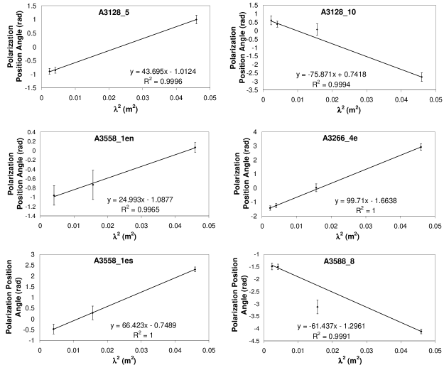
Figure 1: RM fits for the cluster sample examined here. The graph shows the equation of the line where the RM corresponds to the slope, the R² statistic which is a measure of the goodness of fit to a straight line is also given (an R² value of 1 corresponds to a perfect fit, the 13 cm data is given less weight in the fitting due to the poor ATCA off-axis response) .

It should be noted that the use of observations from a period spanning 18 months gives some concern as the data are not all from the same epoch. Nevertheless the quality of the RM fits is excellent and it is therefore assumed that there is no significant variation in the observed source RMs over this time scale.

6 Results: Comparison to Other Data

The RMs obtained from the fitting procedure were then corrected for the contribution from the Galactic rotation measure, G_RM. This was done by using an interpolated all-sky rotation measure map generated from published RM catalogues (Johnston-Hollitt et al. 2004). The Galactic contribution was subtracted from the measured RM to give a residual RM, (RRM) which represents a combination of the cluster RM and the intrinsic source RM. Previous studies have used the standard deviation of the distribution of extra-galactic RMs at high galactic latitudes, beyond the influence of the Galaxy, to argue that the contribution from internal RMs is small. The standard deviation of around 400 extra-galactic RMs at greater than 30 degrees from the Galactic plane was found to be 10 rad m^-2. This suggests that the intrinsic RM component should be small and that RRM should adequately represent the Cluster contribution to the measured RM. Previously it was assumed that the distribution was Gaussian and thus the likelihood of encountering a moderate to high intrinsic RM was very low. However, further analysis of the high Galactic latitude extra-galactic RM population has shown the distribution is exponential at above the 99.9% confidence level. This means that it is more likely to observe a background source with a significant internal contribution to the measured RM than previously thought. This reinforces the requirement to examine cluster magnetic fields statistically.

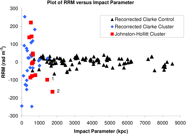
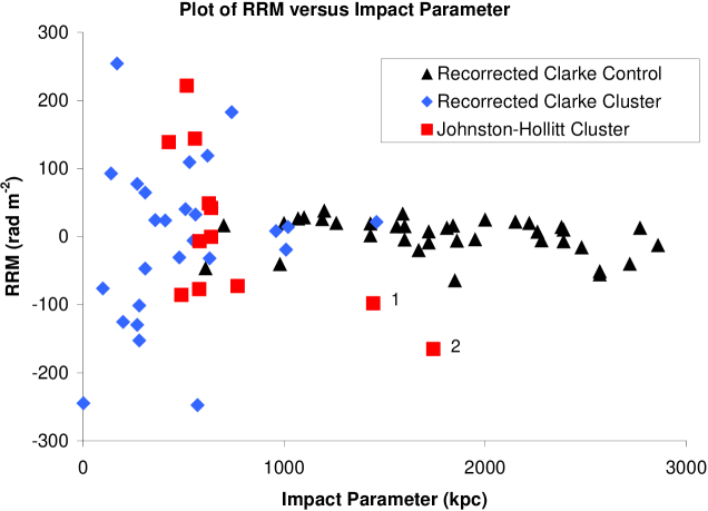
Figure 2: Impact Parameter versus Residual Rotation Measure. The labelled points correspond to sources seen in projection through a region of diffuse synchrotron emission in A3667.

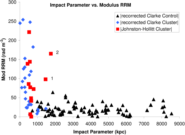
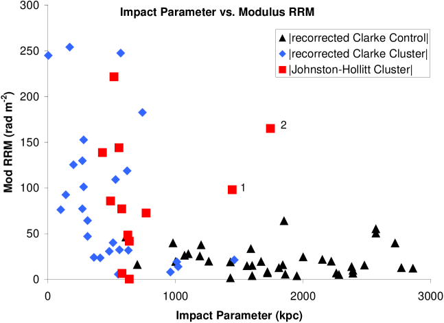
Figure 3: Impact Parameter versus Residual Modulus Rotation Measure. The labelled points correspond to sources seen in projection through a region of diffuse synchrotron emission in A3667.

Clarke (2000) and Clarke et al. (2001) also corrected for the Galactic contribution via examining published RMs in a 15 degree radius about each cluster. In order to directly compare the two datasets, the RRMs from the Clarke (2000) sample were recalculated using the interpolated map. In most cases this made a 5-10% in the RRM values. The two samples were then plotted together on two graphs showing distance from the cluster centre (the so-called impact parameter) versus RRM and $|$RRM$|$. These plots are shown in Figures 2 and 3 respectively. Each plot shows the entire combined dataset out to an impact parameter of 9000 kpc in the top panel and restricted impact parameter range of 0 to 3000 kpc in the lower panel. The RRM of the southern cluster sample presented here (see Table 5) agrees well with the northern sample of Clarke which drops to a background level at around 800 kpc from the cluster core. The two labelled points are both from A3667 and are background sources to the largest and brightest diffuse radio emission region yet discovered (Rottgering et al. 1997; Johnston-Hollitt 2003). These two points are significantly above the RM level suggested by the other data. They are further beyond the region of X-ray emission in A3667 and should fall at a background level, the fact that they do not strongly suggests that these RMs are probing the magnetic field of the diffuse radio emission.

The data for both lobes of the source A3558.1e show quite different RRMs (-0.5 and 41.9) despite being closely spaced. This may either be interpreted as due to tangling of the cluster magnetic field on scales of order of 10 kpc, or as a difference in the internal properties of the radio lobes. Observations of radio jets in low power radio sources have shown that the magnetic field is aligned along the jet and becomes tangled in the resultant lobes due to entrainment. Thus, it is likely here that we are seeing a combination internal and environmental effects.

Table 5: Residual RM corrections. Column 1 gives the source name used in the ATCA observing program and archive; col 2 is the J2000 galactic longitude; col 3 is the J2000 galactic latitude; col 4 is the Galactic contribution to the rotation measure at these co-ordinates as calculated with an interpolated all-sky rotation measure map (Johnston-Hollitt 2004) and col 5 is the residual rotation measure for each source once the Galactic contribution is subtracted.

$$\begin{array}[]{lllll}\vskip 3.0pt plus 1.0pt minus 1.0pt\cr\hrule\cr\vskip 3.0pt plus 1.0pt minus 1.0pt\cr{\rm Source}&{\rm l}&{\rm b}&{\rm G_{RM}}&{\rm RRM}\\ \vskip 3.0pt plus 1.0pt minus 1.0pt\cr\hrule\cr{\rm A}3266\_4{\rm e}&272.29&-40.23&-44.3&144.0\\ {\rm A}3128\_5&262.75&-48.20&-4.9&48.6\\ {\rm A}3128\_10&264.82&-50.91&-3.2&-72.7\\ {\rm A}3558\_1{\rm en}&312.15&30.88&24.5&-0.5\\ {\rm A}3558\_1{\rm es}&312.15&30.88&24.5&41.9\\ {\rm A}3558\_8&312.11&30.62&24.5&-85.9\\ {\rm A}3562\_3&313.37&30.50&29.1&221.6\\ {\rm A}3562\_5&313.52&30.34&26.3&-6.7\\ {\rm A}3571\_3{\rm e}&316.49&28.60&22.2&138.8\\ {\rm A}3667\_{\rm A}&341.32&-33.21&-9.5&-98.2\\ {\rm A}3667\_26{\rm e}&340.98&-33.25&-9.5&-76.7\\ {\rm A}3667\_17&341.19&-32.97&-9.5&-165.1\\ \hrule\cr\end{array}$$

A Kolmogorov-Smirnoff test to assess the likelihood that the combined cluster and the control samples are drawn from the same population was preformed. The test rejected the null hypothesis at greater than 99 precent.

6.1 Embedded versus Background Sources

Recently it has been claimed that the rotation measures of radio sources embedded in clusters are not useful as probes of the global cluster magnetic fields but rather only probe the field local to the source (Rudnick & Blundell 2004). As a counter argument to this we have taken the subsample of those galaxies presented here and in Clarke (2000) which are background to the clusters and performed a Kolmogorov-Smirnoff (KS) test to assess if these data are drawn from the sample population as the control galaxies of Clarke (2000). The KS test rejects the null hypothesis at greater than the 99% confidence level demonstrating that the two samples are not drawn from the same population. We also added the data from Hennessy et al. (1989) to the sample increasing both the cluster and control sample and again per formed a KS test to see if the two samples are drawn from the same population. Again the null hypothesis can be rejected at over 99% confidence. In addition, we also considered the hypothesis that the RMs derived from embedded and background sources might be drawn from the same population. In this case the null hypothesis could not be rejected and it seems, that statistically speaking at least, there is no difference in the value of RMs derived from background or embedded cluster sources seen in project through galaxy clusters. Thus, despite concerns over the validity of the embedded galaxies as probes there is no statistical evidence this class of source gives rise to significantly different RMs to background galaxies though both a combined embedded and cluster background sample gives rises to a significantly different RMs than the control sample. Further, even using only background sources there is a still statistically significant excess RM detected along lines of sight through X-ray luminous clusters when compared with other lines of sight. With the exception of the points in A3667, our data agree well with the previous samples and support the finding by Clarke (2000) and show an excess RM toward the centre of galaxy clusters. We find the combined cluster RM sample of Clarke (2000), Hennessy et al. (1989) and these data has a standard deviation of $\sigma_{RM}$ = 125 rad m^-2. In comparison, the standard deviation of a sample of 474 extra-galactic sources at least 30 degrees from the galactic plane gave $\sigma$ =10 rad m^-2 (Johnston-Hollitt 2003).

7 Conclusion

We have presented the results of a search to detected excess Faraday rotation toward the cores of several southern, non-cooling flow clusters. We find that the population of RMs derived from combined sample of data from this work and the literature through lines of sight through galaxy clusters is statistically different to RMs from other lines of sight. Further, we find that this holds even for a sample of only background galaxies seen in projection through clusters. Additionally, a comparison of data from embedded and background sources can not reject the null hypothesis that the values are drawn from the same population. In conclusion we argue that the results of this study agree well with those of Clarke (2000), supporting the notion that a statistically significant broadening of the RM distribution is measured out to around 800 kpc for nearby galaxy clusters. This suggests cluster magnetic fields to be of the order of 1–2 $\mu$G assuming a tangled cell model.

References

- Broten et al. (1988) Broten, N. W., MacLeod, J. M., & Vallee, J. P. 1988, Ap&SS, 141, 303
- Burbidge (1958) Burbidge, G. R. 1958, ApJ, 128, 1
- Burkard (1961) Burkard, O. 1961, J. Geophys. Res., 66, 3058
- Clarke (2000) Clarke, T. E. 2000, Ph.D. Thesis
- Clarke et al. (2001) Clarke, T. E., Kronberg, P. P., & Böhringer, H. 2001, ApJ, 547, L111
- Cooper & Price (1962) Cooper, B. F. C. & Price, R. M. 1962, Nature, 195, 1084
- Dennison (1979) Dennison, B. 1979, AJ, 84, 725
- Ebeling et al. (1996) Ebeling, H., Voges, W., Bohringer, H., et al. 1996, MNRAS, 281, 799
- Goldshmidt & Rephaeli (1993) Goldshmidt, O. & Rephaeli, Y. 1993, ApJ, 411, 518
- Hennessy et al. (1989) Hennessy, G. S., Owen, F. N., & Eilek, J. A. 1989, ApJ, 347, 144
- Jaffe (1980) Jaffe, W. 1980, ApJ, 241, 925
- Johnston-Hollitt (2003) Johnston-Hollitt, M. 2003, Ph.D. Thesis
- Johnston-Hollitt (2004) Johnston-Hollitt, M. 2004, in The Riddle of Cooling Flows in Galaxies and Clusters of galaxies
- Johnston-Hollitt et al. (2004) Johnston-Hollitt, M., Hollitt, C. P., & Ekers, R. D. 2004, in The Magnetized Interstellar Medium, 13–18
- Kim (1988) Kim, K. 1988, Ph.D. Thesis
- Kim et al. (1990) Kim, K.-T., Kronberg, P. P., Dewdney, P. E., & Landecker, T. L. 1990, ApJ, 355, 29
- Kim et al. (1991) Kim, K.-T., Kronberg, P. P., & Tribble, P. C. 1991, ApJ, 379, 80
- Kronberg & Simard-Normandin (1976) Kronberg, P. P. & Simard-Normandin, M. 1976, Nature, 263, 653
- Lawler & Dennison (1982) Lawler, J. M. & Dennison, B. 1982, ApJ, 252, 81
- Rottgering et al. (1997) Rottgering, H. J. A., Wieringa, M. H., Hunstead, R. W., & Ekers, R. D. 1997, MNRAS, 290, 577
- Rudnick & Blundell (2004) Rudnick, L. & Blundell, K. M. 2004, in The Riddle of Cooling Flows in Galaxies and Clusters of galaxies
- Sault et al. (1995) Sault, R. J., Teuben, P. J., & Wright, M. C. H. 1995, in ASP Conf. Ser. 77: Astronomical Data Analysis Software and Systems IV, 433–+
- Simard-Normandin et al. (1981) Simard-Normandin, M., Kronberg, P. P., & Button, S. 1981, ApJS, 45, 97
- Taylor et al. (1994) Taylor, G. B., Barton, E. J., & Ge, J. 1994, AJ, 107, 1942
- Vallee (1990) Vallee, J. P. 1990, ApJ, 360, 1
- Vallee et al. (1986) Vallee, J. P., MacLeod, M. J., & Broten, N. W. 1986, A&A, 156, 386
- Welter et al. (1984) Welter, G. L., Perry, J. J., & Kronberg, P. P. 1984, ApJ, 279, 19