The scale-dependence of relative galaxy bias:
encouragement for the “halo model” description

Abstract

We investigate the relationship between the colors, luminosities, and environments of galaxies in the Sloan Digital Sky Survey spectroscopic sample, using environmental measurements on scales ranging from $0.2$ to $6$ $h^{-1}$ Mpc. We find: (1) that the relationship between color and environment persists even to the lowest luminosities we probe ($M_{r}-5\log_{10}h\sim-14$); (2) at luminosities and colors for which the galaxy correlation function has a large amplitude, it also has a steep slope; and (3) in regions of a given overdensity on small scales (1 $h^{-1}$ Mpc), the overdensity on large scales (6 $h^{-1}$ Mpc) does not appear to relate to the recent star formation history of the galaxies. Of these results, the last has the most immediate application to galaxy formation theory. In particular, it lends support to the notion that a galaxy’s properties are related only to the mass of its host dark matter halo, and not to the larger scale environment.

1 Motivation

Recent investigations of the large scale distribution of galaxies in the Sloan Digital Sky Survey (SDSS; Abazajian et al. 2004) have revealed a complex relationship between the properties of galaxies, (such as color, luminosity, surface brightness, and concentration) and their environments (Hogg et al. 2003; Blanton et al. 2004a; Berlind et al. 2004). These and other investigations using the SDSS (Zehavi et al. 2002, 2004; Kauffmann et al. 2004) and the Two-degree Field Galaxy Redshift Survey (Norberg et al. 2002; Balogh et al. 2004) have found that galaxy clustering is a function both of star formation history and of luminosity. For low luminosity galaxies, clustering is a strong function of color, while for luminous galaxies clustering is a strong function of luminosity. For red galaxies, clustering is a non-monotonic function of luminosity, peaking at both high and low luminosities. Although galaxy clustering correlates also with surface brightness and concentration, Blanton et al. (2004a) and Kauffmann et al. (2004) show that galaxy environment is independent of these properties at fixed color and luminosity. Thus, color and luminosity — measures of star formation history — appear to have a more fundamental relationship with environment than do surface brightness and concentration — measures of the distribution of stars within the galaxy.

Some of the investigations above have explored the scale dependence of these relationships. Studies of the correlation function, such as Norberg et al. (2002) and Zehavi et al. (2004), can address this question, but do not address directly whether the density on large scales is related to galaxy properties independent of the relationships with density on small scales. If only the masses of the host halos of galaxies strongly affect their properties, then we expect no such independent relationship between galaxy properties and the large scale density field. Thus, it is important to examine this issue in order to test the assumptions of the “halo model” description of galaxy formation and of semi-analytic models that depend only on the properties of the host halo (e.g., Kauffmann et al. 1993; Seljak 2000; White et al. 2001; Berlind & Weinberg 2002). Recent studies of this question have come to conflicting conclusions. For example, Balogh et al. (2004) have concluded from their analysis of SDSS and 2dFGRS galaxies that the equivalent width of H$\alpha$ is a function of environment measured on scales of 1.1 $h^{-1}$ Mpc and 5.5 $h^{-1}$ Mpc independently of each other. On the other hand, Kauffmann et al. (2004) find that at fixed density at scales of 1 $h^{-1}$ Mpc, the distribution of D4000 (a measure of the age of the stellar population) is not a strong function of density on larger scales.

Here we address the dependence on scale of the relative bias of SDSS galaxies. Section 2 describes our data set. Section 3 explores how the relationship between the color, luminosity, and environments of galaxies depends on scale. Section 4 resolves the discrepancy noted in the previous paragraph between Kauffmann et al. (2004) and Balogh et al. (2004), finding that only small scales are important to the recent star formation history of galaxies. Section 5 summarizes the results.

Where necessary, we have assumed cosmological parameters $\Omega_{0}=0.3$, $\Omega_{\Lambda}=0.7$, and $H_{0}=100h$ km s^-1 Mpc^-1 with $h=1$.

2 Data

2.1 SDSS

The SDSS is taking $ugriz$ CCD imaging of $10^{4}~{}\mathrm{deg^{2}}$ of the Northern Galactic sky, and, from that imaging, selecting $10^{6}$ targets for spectroscopy, most of them galaxies with $r<17.77~{}\mathrm{mag}$ (e.g., Gunn et al., 1998; York et al., 2000; Abazajian et al., 2003). Automated software performs all of the data processing: astrometry (Pier et al., 2003); source identification, deblending and photometry (Lupton et al., 2001); photometricity determination (Hogg et al., 2001); calibration (Fukugita et al., 1996; Smith et al., 2002); spectroscopic target selection (Eisenstein et al., 2001; Strauss et al., 2002; Richards et al., 2002); spectroscopic fiber placement (Blanton et al., 2003); and spectroscopic data reduction. An automated pipeline called idlspec2d measures the redshifts and classifies the reduced spectra (Schlegel et al., in preparation).

The spectroscopy has small incompletenesses coming primarily from (1) galaxies missed because of mechanical spectrograph constraints (6 percent; Blanton et al., 2003), which leads to a slight under-representation of high-density regions, and (2) spectra in which the redshift is either incorrect or impossible to determine ($<1$ percent). In addition, there are some galaxies ($\sim 1$ percent) blotted out by bright Galactic stars, but this incompleteness should be uncorrelated with galaxy properties.

2.2 NYU-VAGC

For the purposes of computing large-scale structure and galaxy property statistics, we have assembled a subsample of SDSS galaxies known as the NYU Value Added Galaxy Catalog (NYU-VAGC; Blanton et al. 2004b). One of the products of that catalog is a low redshift catalog. Here we use the version of that catalog corresponding to the SDSS Data Release 2 (DR2).

The low redshift catalog has a number of important features which are useful in the study of low luminosity galaxies. Most importantly:

1. We have checked by eye all of the images and spectra of low luminosity ($M_{r}-5\log_{10}h>-15$) or low redshift ($z<0.01$) galaxies in the NYU-VAGC. Most significantly, we have trimmed those which are “flecks” incorrectly deblended out of bright galaxies; for some of these cases, we have been able to replace the photometric measurements with the measurements of the parents. For a full description of our checks, see Blanton et al. (2004b).

2. For galaxies which were shredded in the target version of the deblending, the spectra are often many arcseconds away from the nominal centers of the galaxy in the latest version of the photometric reductions. We have used the new version of the deblending to decide whether these (otherwise non-matched spectra) should be associated with the galaxy in the best version.

3. We have estimated the distance to low redshift objects using the Willick et al. (1997) model of the local velocity field (using $\beta=0.5$), and propagated the uncertainties in distance into uncertainties in absolute magnitude.

For the purposes of our analysis below, we have matched this sample to the results of Tremonti et al. (2004), who measured emission line fluxs and equivalent widths for all of the SDSS spectra. Below, we use their results for the H$\alpha$ equivalent width.

The range of distances we include is $10<d<150$ $h^{-1}$ Mpc, making the sample volume limited for galaxies with $M_{r}-5\log_{10}h<-18.5$. The total completeness-weighted effective area of the sample, excluding areas close to Tycho stars, is 2220.9 square degrees. The catalog contains 28,089 galaxies. Blanton et al. (2004c) have investigated the luminosity function, surface brightness selection effects, and galaxy properties in this sample.

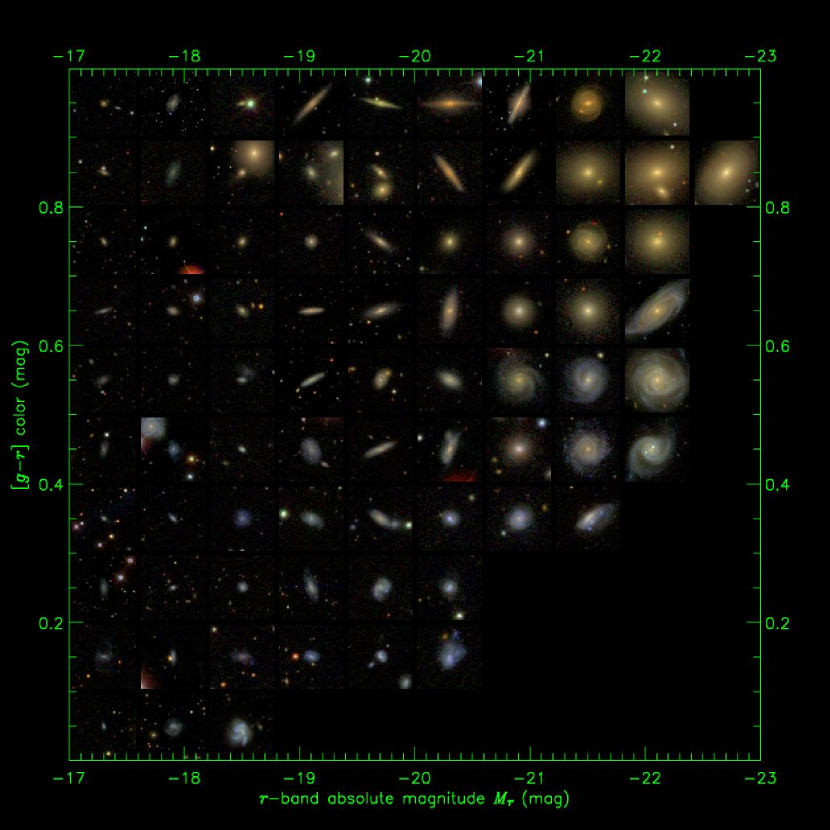
Figure 1: In each bin of color and absolute magnitude, we show a randomly chosen SDSS galaxy image. Each image is 40 $h^{-1}$ kpc on a size.

We will be studying the environments of galaxies as a function of their luminosity and color below. To give a sense of the morphological properties of galaxies with various luminosities and colors, Figure 1 shows galaxies randomly selected in bins of color and luminosity. Each image is 40 $h^{-1}$ kpc on a side. Red, high luminosity galaxies are classic giant ellipticals. Lower luminosity red galaxies tend to be more flattened and less concentrated. Blue, high luminosity galaxies have well-defined spiral structure and dust lanes. Lower luminosity blue galaxies have less well-defined bulges and fewer spiral features.

2.3 Densities

In order to evaluate the environments of galaxies in our sample, we perform the following procedure.

First, for each given galaxy in the sample, we count the number of other galaxies $N_{i}$ with $M_{r}-5\log_{10}h<-18.5$ outside a projected radius of 10 $h^{-1}$ kpc and within some outer radius $r_{T}$, which we will vary below, and within $\pm 1000$ km s^-1 in the redshift direction. This trace catalog is volume-limited within $z<0.05$. In order to make a more direct comparison to Balogh et al. (2004), we will also use a trace catalog containing only galaxies with $M_{r}-5\log_{10}h<-20.5$.

Second, we calculate the mean expected number of galaxies in that volume as:

$$N_{\mathrm{exp},i}={\bar{n}}\int\,dVf(\alpha,\delta)$$ (1)

where $f(\alpha,\delta)$ is the sampling fraction of galaxies in the right ascension ($\alpha$) and declination ($\delta$) direction of each point within the volume. We perform this integral using a Monte Carlo approach, distributing random points inside the volume with a density modulated by the sampling fraction $f(\alpha,\delta)$.

In order to calculate the mean density around galaxies in various classes, we will simply calculate:

$$1+\delta=\frac{\sum_{i}N_{i}}{\sum_{i}N_{\mathrm{exp},i}}$$ (2)

as the density with respect to the mean.

3 Dependence of mean density on color and luminosity

When one calculates the mean density around galaxies, it is necessary to have a fair sample of the universe. For the most luminous galaxies in our sample ($M_{r}-5\log_{10}h<-18.5$) the sample is volume-limited out to our redshift limit of $z=0.05$ and constitutes the equivalent of a 60 $h^{-1}$ Mpc radius sphere, which constitutes a fair sample for many purposes ($\Lambda$CDM predicts a variance in such a sphere to be about 0.13). However, the lower luminosity galaxies can only be seen in the fraction of this volume which is nearby, and below a certain luminosity the sample is no longer fair. For example, consider Figure 2, which shows the cumulative mean density around galaxies with $M_{r}-5\log_{10}h<-18.5$ in spheres of larger and larger radius around the Milky Way. The mean overdensity does not converge until a volume which corresponds to approximately $z=0.03$. Thus, it is not really safe to evaluate the mean density around galaxies that are too low luminosity to be observed out that far in redshift, which is to say, less luminous than $M_{r}-5\log_{10}h=-17$.

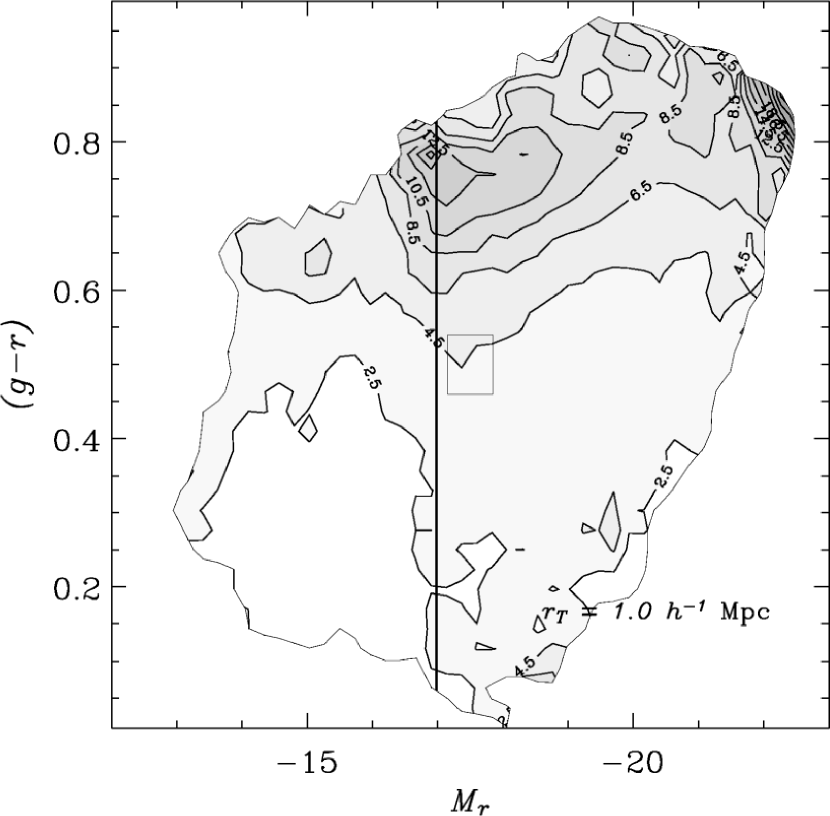
Figure 3: Mean density $\delta(M_{r},g-r)+1$ around galaxies using $r_{T}=1$ $h^{-1}$ Mpc. As found in Hogg et al. (2003) and Blanton et al. (2004a), there is a strong increase in the mean density around luminous galaxies as a function of luminosity, and around blue galaxies as a function of color. The solid line indicates the minimum luminosity for which our sample constitutes a fair sample (to the left of this line the mean density of galaxies is underestimated).

However, for the moment let us consider Figure 3. The greyscale and contours show the mean density relative to the mean as a function of color and luminosity, using a projected radius of $0.5$ $h^{-1}$ Mpc. The mean is calculated in a sliding box with the width shown. If the sliding box contains fewer than 20 galaxies, the result is ignored and colored pure white. Here we show the results for the entire sample. Our statistical uncertainties are well-behaved down to about $M_{r}-5\log_{10}h\sim-14.5$, but we are likely to be cosmic variance limited for $M_{r}-5\log_{10}h>-17$, as indicated by the solid vertical line. Thus, the apparent decline in the mean overdensity for red galaxies lower luminosity than $M_{r}-5\log_{10}h\sim-17$ is probably spurious. Despite that limitation, we note that there is a strong relationship between environment and color even at $M_{r}-5\log_{10}h\sim-15$.

We note in passing that we can still use the variation of the density within $z<0.03$ to study the properties of galaxies as a function of density down to low luminosity. Just because the mean density of galaxies in that volume has not converged does not imply that there is insufficient variation of density to study the variation of galaxy properties with environment.

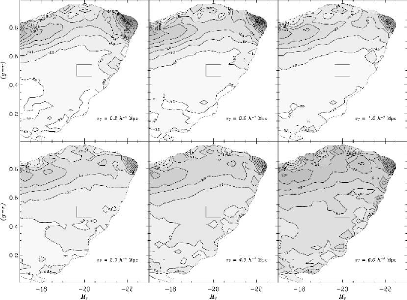
Figure 4: Similar to Figure 3, now limited to $M_{r}<-17$, and showing six different scales.

For our fair sample of galaxies with $M_{r}-5\log_{10}h<-17$, Figure 4 shows the dependence of overdensity on luminosity and color for six different projected radii: 0.2, 0.5, 1, 2, 4, and 6 $h^{-1}$ Mpc. We only show results for $M_{r}-5\log_{10}h<-17$, for which we have a fair sample. Obviously, the density contrast decreases with scale; on the other hand, the qualitative form of the plot does not change.

Our results remain similar to those shown in Hogg et al. (2003) and Blanton et al. (2004a). The results here demonstrate that the environments of low luminosity, red galaxies do continue to become denser as absolute magnitude increases down to absolute magnitudes of $-17$ (about two magnitudes less luminous than explored by our previous work).

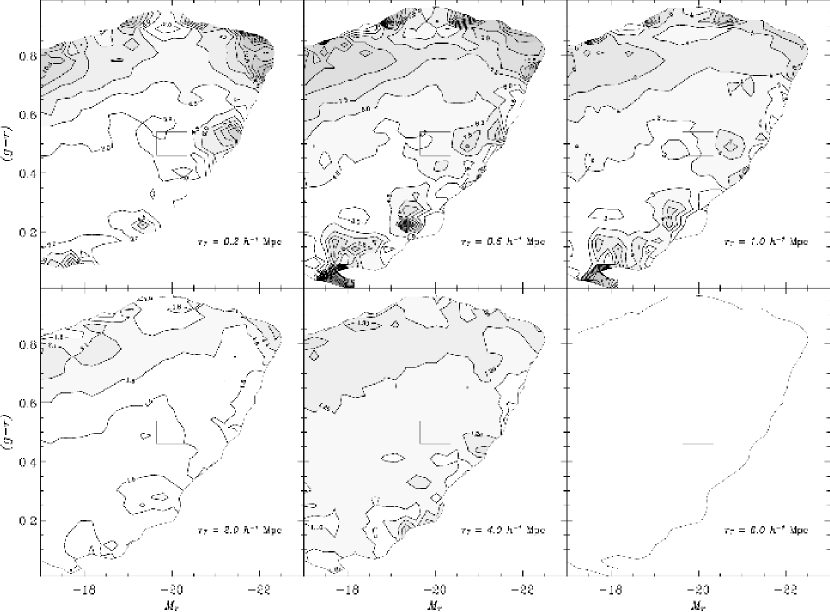
Figure 5: Similar to Figure 4, but showing the ratio of the overdensity $\delta(M_{r},g-r)$ at each scale to that at $r_{T}=6$ $h^{-1}$ Mpc. Thus, the bottom right panel is unity across the entire plot. This ratio is a measure of the steepness of the correlation function at each absolute magnitude and color. Interestingly, the contours of steepness are similar to the contours in overdensity at any scale, meaning that wherever the local density at $r_{T}=6.0$ $h^{-1}$ Mpc is higher, the correlation function is also steeper.

Figure 5 shows the ratio of the overdensity $\delta$ at each scale relative to that at the largest scale of $r_{T}=6$ $h^{-1}$ Mpc. This ratio is a measure of the steepness of the cross-correlation between galaxies of a given color and absolute magnitude with all galaxies in our volume-limited sample ($M_{r}-5\log_{10}h<-18.5$). Interestingly, the contours in steepness are qualitatively similar to the contours in overdensity in Figure 4. This similarity implies that for each class of galaxy, the strength of the correlation on large scales always is associated with a steeper correlation function.

4 Blue fraction as a function of environment

Another way of looking at similar results is to ask, as a function of environment, what fraction of galaxies are blue. We split the sample into “red” and “blue” galaxies using the following, luminosity-dependent cut:

$$(g-r)_{c}=0.65-0.03(M_{r}-5\log_{10}h+20)$$ (3)

Blue galaxies thus have $(g-r)<(g-r)_{c}$. We then sort all the galaxies with $M_{r}-5\log_{10}h<-18.5$ into bins of density on three different scales: $r_{T}=0.5$, $1.0$, and $6.0$ $h^{-1}$ Mpc. In each bin we calculate the fraction of blue galaxies. Figure 6 shows this blue fraction as a function of density. In all cases, the blue fraction declines as a function of density, as one would expect based on Figure 4 above, and from the astronomical literature (a highly abridged list of relevant work would include Hubble 1936; Oemler 1974; Dressler 1980; Hermit et al. 1996; Guzzo et al. 1997; Giuricin et al. 2001; Hashimoto & Oemler 1999; Norberg et al. 2002; Zehavi et al. 2004). If we divide the sample into bins of luminosity, we find that higher luminosities have smaller blue fractions (of course) but that the dependence of blue fraction on density does not change.

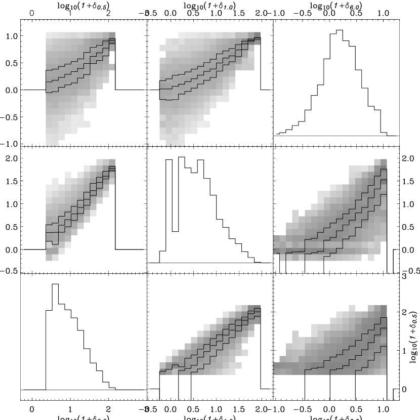
Figure 7: Comparison of density estimates on different scales. Diagonal plots show the distribution of density estimates on scales of $r_{T}=0.5$, $1.0$, and $6.0$ $h^{-1}$ Mpc. Off-diagonal plots show as a greyscale the conditional distribution of each density estimate with respect to all the others. The lines show the quartiles of the distribution. Generally speaking, a larger density on one scale indicates a larger density on all other scales. Obviously, the correlation is stronger for scales closer to one another. Note that while a large density for $r_{T}=0.5$ $h^{-1}$ Mpc implies a large density for $r_{T}=6.0$ $h^{-1}$ Mpc, the opposite is not the case: there is a large range of densities on the smaller scale given any value of the density on the larger scale.

The question naturally arises: which scales are important to the process of galaxy formation? Is the local environment within 0.5 $h^{-1}$ Mpc the only important consideration? Or is the larger scale environment also important? For example, consider Figure 7, which shows the conditional dependence of the three density estimators at the three scales on each other. The diagonal plots simply show the distribution within our sample of each density estimator. The off-diagonal plots show the conditional distribution of the quantity on the $y$-axis given the quantity on the $x$-axis. As an example, the lower right panel shows $P\left(\log_{10}(1+\delta_{0.5})|\log_{10}(1+\delta_{6.0})\right)$. The lines are the quartiles of the distribution. Obviously, the estimators are correlated with one another; thus, a dependence of blue fraction on one on them is likely to cause a dependence of blue fraction on any of the density estimators. However, physically, our theoretical expectation is that the density on smaller scales is more important than that on larger scales. That is, for a given density on small scales, we expect that the density on much larger scales (much larger than the size of the largest virialized dark matter halos) should not be closely related to the properties of the galaxies. To address this question, we ask what the blue fraction is as a function of density measurements on two different scales.

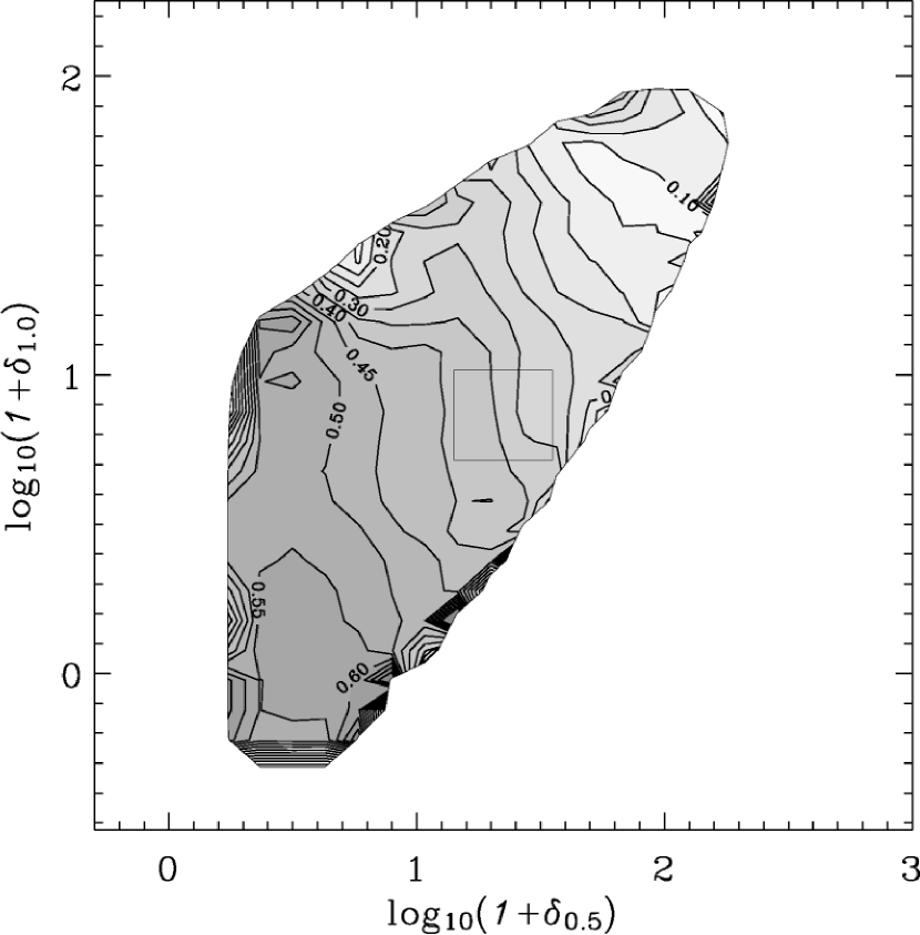
Figure 8: Contours and greyscale show the blue galaxy fraction as a function of local density on $r_{T}=0.5$ and $1$ $h^{-1}$ Mpc scales. The local density on both scales is important.

Figure 8 shows the fraction of blue galaxies as a function of two density estimates: one with $r_{T}=0.5$ $h^{-1}$ Mpc and one with $r_{T}=1.0$ $h^{-1}$ Mpc . In this case it is clear that the blue fraction is a function of both densities. That is, even at a fixed density on scales of $0.5$ $h^{-1}$ Mpc, the density outside that radius matters to the blue fraction; in addition, at a fixed density on scales of $1.0$ $h^{-1}$ Mpc, the distribution of galaxies within that radius appears to affect the blue fraction as well.

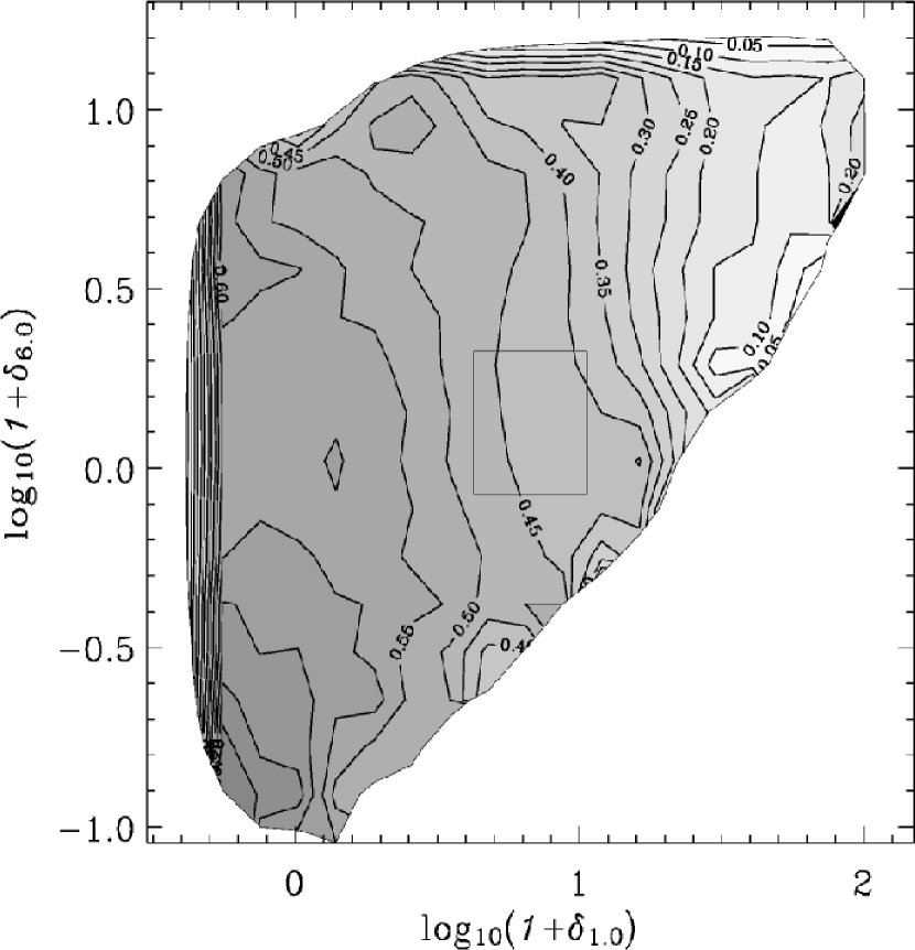
Figure 9: Contours and greyscale show the blue galaxy fraction as a function of local density on $r_{T}=1$ and $6$ $h^{-1}$ Mpc scales. The vertical contours demonstrate that only the local density on the smaller scale is important.

On the other hand, consider Figure 9, which is the same as Figure 8, but now showing the densities at scales of $r_{T}=1.0$ and $6.0$ $h^{-1}$ Mpc. In Figure 9 the contours are vertical, indicating that the density between $1.0$ and $6.0$ $h^{-1}$ Mpc has very little effect on galaxy properties. At a fixed value of the density at the smaller scale, the larger scale environment appears to be of little importance.

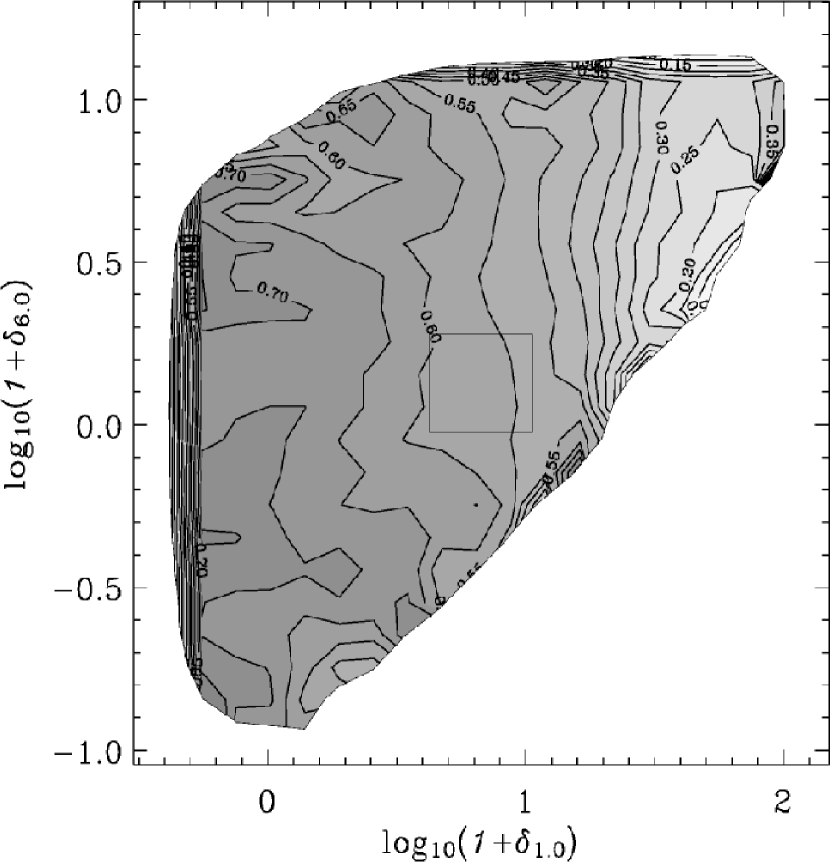
Figure 10: Similar to Figure 9, but for the H$\alpha$ emitting fraction rather than the blue fraction. Again, only the small scales are important.

Balogh et al. (2004) found that these contours were not vertical when he looked at the fraction of galaxies for which the H$\alpha$ equivalent width was $>4$ Å. Their result appears in conflict with that of the previous paragraph. On the other hand, the emission lines measure a more recent star formation rate than does the color; it is possible in principle that the more recent star formation rate depends more strongly on large-scale environment. To rule out this possibility, Figure 10 shows the same result as Figure 9, but now showing the fraction of galaxies with H$\alpha$ equivalent widths (as measured by Tremonti et al. 2004) greater than 4 Å. Again, for strong emission line fraction as for the blue fraction, the smaller scales are important, but the 6 $h^{-1}$ Mpc scales are not, in contradiction with Balogh et al. (2004).

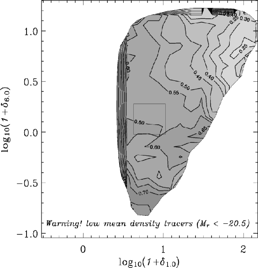
Figure 11: Similar to Figure 10, but (for comparison with Balogh et al. 2004) using galaxies with $M_{r}<-20.5$ as tracers rather than galaxies with $M_{r}<-18.5$. With these tracers, the large scale density field yields extra information not contained in the small scale density field, probably because there is effectively “noise” in the relationship between the brighter, lower mean density tracers and the underlying density field which determines the properties of the galaxy population.

Why, then, did Balogh et al. (2004) conclude that large scales were important? There are a number of differences between our study and theirs. First, their contouring method differs; instead of measuring the blue fraction in bins of fixed size, at each point they measure the star-forming fraction among the nearest 500 galaxies in the plane of $\delta_{1.1}$ and $\delta_{5.5}$. We have found that this procedure creates a slight bias in the contouring in the sense that near the edges of the distribution vertical contours will become diagonal. However, this effect is not strong enough to explain the differences between our results and those of Balogh et al. (2004). Second, to estimate the density in their sample they used a spherical Gaussian filter, whereas here we use the overdensity in cones. We have not investigated what effect this difference has. Finally, they use tracer galaxies with a considerably lower mean density than ours. Their effective absolute magnitude limit is $M_{r}-5\log_{10}h<-20.5$; such galaxies have a mean density of $\sim 4.0\times 10^{-3}$ $h^{3}$ Mpc^-3. Our tracers ($M_{r}-5\log_{10}h<-18.5$) have a mean density of $\sim 2.3\times 10^{-2}$ $h^{3}$ Mpc^-3, almost six times higher. Figure 11 shows our results when we restrict our tracer sample to $M_{r}-5\log_{10}h<-20.5$. The contours in this figure are very diagonal, similar to the results of Balogh et al. (2004).

This result suggests that one of two possible mechanisms are causing the differences between our results and those of Balogh et al. (2004). First, the higher luminosity galaxies with $M_{r}-5\log_{10}h<-20.5$ might be yielding fundamentally different information about the density field than our lower luminosity tracers. Second, the lower mean density of the galaxies with $M_{r}-5\log_{10}h<-20.5$ might be effectively introducing “noise” in the measurement on small scales. Remember that the large scale and small scale densities are intrinsically correlated. So if the small scale measurement is noisy enough, the higher signal-to-noise ratio large scale measurement could actually be adding extra information about the environment on small scales. Such an effect would make the contours in Figure 11 diagonal. We have performed a simple test to distinguish these possibilities, which is to remake Figure 10 using the low luminosity tracers ($M_{r}-5\log_{10}h<-18.5$) but subsampling them to the same mean density as the high luminosity tracers ($M_{r}-5\log_{10}h<-20.5$). This test yields diagonal contours, meaning one can understand the diagonal contours of Figure 11 and of Balogh et al. (2004) as simply reflecting the low signal-to-noise ratio of the density estimates.

5 Summary and Discussion

We explore the relative bias between galaxies as a function of scale, finding the following.

1. The dependence of mean environment on color persists to the lowest luminosities we explore ($M_{r}-5\log_{10}h\sim-14$).

2. Red, low luminosity galaxies tend to be in overdense regions, down at least to $M_{r}-5\log_{10}h\sim-17$. This result extends those found by Hogg et al. (2003) and Blanton et al. (2004a) towards lower luminosities by about 2 magnitudes.

3. At any given point of color and luminosity, a correlation function with a stronger amplitude implies correlation function with a steeper slope.

4. In regions of a given overdensity on small scales ($r_{T}=1$ $h^{-1}$ Mpc), the overdensity on large scales ($r_{T}=6$ $h^{-1}$ Mpc) does not appear to relate to the recent star formation history of the galaxies.

The last point above deserves elaboration. First, it contradicts the results of Balogh et al. (2004). We have found that their results are probably due to the low mean density of the tracers they used. This explanation underscores the importance of taking care when using low signal-to-noise quantities. Galaxy environments are difficult to measure, in the sense we use tracers that do not necessarily trace the “environment” perfectly, meaning neither with low noise nor necessarily in an unbiased manner. We claim here that our higher density of tracers marks an improvement over previous work, but it is worth noting the limitations of assuming that the local galaxy density fairly and adequately represents whatever elements of the environment affect galaxy formation.

Second, if the galaxy density field is an adequate representation of the environment, the result has important implications regarding the physics of galaxy formation. In simulations whose initial conditions are constrained by cosmic microwave background observations and galaxy large-scale structure observations, virialized dark matter halos do not extend to sizes much larger than $1$–$2$ $h^{-1}$ Mpc. Thus, our results are consistent with the notion that only the masses of the host halos of the galaxies we observe are strongly affecting the star formation of the galaxies. In addition, Blanton et al. (2004a) find that only the star formation histories, not the azimuthally-averaged structural parameters, are directly related to environment. For these reasons, it is likely that we can understand the process of galaxy formation by only considering the properties of the host dark matter halos. Our results therefore encourage the “halo model” description of galaxy formation and the pursuit of semi-analytic models which depend only on the properties of the host halo (e.g., Kauffmann et al. 1997; Seljak 2000; Benson et al. 2001; White et al. 2001; Berlind & Weinberg 2002).

Figure 2: Mean density $\delta+1$ on scales $r_{T}=1.0$ $h^{-1}$ Mpc around galaxies with $M_{r}<-18.5$ for galaxies at redshifts $<z$, as a function of enclosed volume in the sample $V(z)$ (in units of $h^{-3}$ Mpc³). The mean is calculated in a sliding box with the width shown. If the sliding box contains fewer than 20 galaxies, the result is colored pure white. Such galaxies are observable out to $z=0.05$, the limit of this plot. The mean density of such galaxies converges at $z=0.03$.

Figure 6: Fraction of blue galaxies (using the definition of Equation 3) as a function of local density on three different scales, as labeled. Uncertainties are Poisson estimates (not binomial). The dotted line represents the blue fraction for all galaxies with no neighbors.

References

- Abazajian et al. (2003) Abazajian, K. et al. 2003, AJ, 126, 2081
- Abazajian et al. (2004) Abazajian, K. et al. 2004, AJ, 128, 502
- Balogh et al. (2004) Balogh, M., Eke, V., Miller, C., Lewis, I., Bower, R., Couch, W., Nichol, R., Bland-Hawthorn, J., Baldry, I. K., Baugh, C., Bridges, T., Cannon, R., Cole, S., Colless, M., Collins, C., Cross, N., Dalton, G., de Propris, R., Driver, S. P., Efstathiou, G., Ellis, R. S., Frenk, C. S., Glazebrook, K., Gomez, P., Gray, A., Hawkins, E., Jackson, C., Lahav, O., Lumsden, S., Maddox, S., Madgwick, D., Norberg, P., Peacock, J. A., Percival, W., Peterson, B. A., Sutherland, W., & Taylor, K. 2004, MNRAS, 348, 1355
- Benson et al. (2001) Benson, A. J., Frenk, C. S., Baugh, C. M., Cole, S., & Lacey, C. G. 2001, MNRAS, 327, 1041
- Berlind et al. (2004) Berlind, A. A., R., B. M., Hogg, D. W., Weinberg, D. H., Davé, R., Eisenstein, D. J., & Katz, N. 2004, ApJ, submitted (astro-ph/0406633)
- Berlind & Weinberg (2002) Berlind, A. A. & Weinberg, D. H. 2002, ApJ, 575, 587
- Blanton et al. (2004a) Blanton, M. R., Eisenstein, D. J., Hogg, D. W., Schlegel, D. J., & Brinkmann, J. 2004a, ApJ, in press (astro-ph/0310453)
- Blanton et al. (2003) Blanton, M. R., Lin, H., Lupton, R. H., Maley, F. M., Young, N., Zehavi, I., & Loveday, J. 2003, AJ, 125, 2276
- Blanton et al. (2004b) Blanton, M. R. et al. 2004b, in preparation
- Blanton et al. (2004c) Blanton, M. R. et al. 2004c, in preparation
- Dressler (1980) Dressler, A. 1980, ApJ, 236, 351
- Eisenstein et al. (2001) Eisenstein, D. J. et al. 2001, AJ, 122, 2267
- Fukugita et al. (1996) Fukugita, M., Ichikawa, T., Gunn, J. E., Doi, M., Shimasaku, K., & Schneider, D. P. 1996, AJ, 111, 1748
- Giuricin et al. (2001) Giuricin, G., Samurović, S., Girardi, M., Mezzetti, M., & Marinoni, C. 2001, ApJ, 554, 857
- Gunn et al. (1998) Gunn, J. E., Carr, M. A., Rockosi, C. M., Sekiguchi, M., et al. 1998, AJ, 116, 3040
- Guzzo et al. (1997) Guzzo, L., Strauss, M. A., Fisher, K. B., Giovanelli, R., & Haynes, M. P. 1997, ApJ, 489, 37
- Hashimoto & Oemler (1999) Hashimoto, Y. & Oemler, A. J. 1999, ApJ, 510, 609
- Hermit et al. (1996) Hermit, S., Santiago, B. X., Lahav, O., Strauss, M. A., Davis, M., Dressler, A., & Huchra, J. P. 1996, MNRAS, 283, 709
- Hogg et al. (2001) Hogg, D. W., Finkbeiner, D. P., Schlegel, D. J., & Gunn, J. E. 2001, AJ, 122, 2129
- Hogg et al. (2003) Hogg, D. W. et al. 2003, ApJ, 585, L5
- Hubble (1936) Hubble, E. P. 1936, The Realm of the Nebulae (New Haven: Yale University Press)
- Kauffmann et al. (1997) Kauffmann, G., Nusser, A., & Steinmetz, M. 1997, MNRAS, 286, 795
- Kauffmann et al. (1993) Kauffmann, G., White, S. D. M., & Guiderdoni, B. 1993, MNRAS, 264, 201
- Kauffmann et al. (2004) Kauffmann, G., White, S. D. M., Heckman, T. M., Ménard, B., Brinchmann, J., Charlot, S., Tremonti, C., & Brinkmann, J. 2004, MNRAS, 314
- Lupton et al. (2001) Lupton, R. H., Gunn, J. E., Ivezić, Z., Knapp, G. R., Kent, S., & Yasuda, N. 2001, in ASP Conf. Ser. 238: Astronomical Data Analysis Software and Systems X, Vol. 10, 269
- Norberg et al. (2002) Norberg, P. et al. 2002, MNRAS, 332, 827
- Oemler (1974) Oemler, A. 1974, ApJ, 194, 1
- Pier et al. (2003) Pier, J. R., Munn, J. A., Hindsley, R. B., Hennessy, G. S., Kent, S. M., Lupton, R. H., & Ivezić, Ž. 2003, AJ, 125, 1559
- Richards et al. (2002) Richards, G. et al. 2002, AJ, 123, 2945
- Seljak (2000) Seljak, U. 2000, MNRAS, in press
- Smith et al. (2002) Smith, J. A., Tucker, D. L., et al. 2002, AJ, 123, 2121
- Strauss et al. (2002) Strauss, M. A. et al. 2002, AJ, 124, 1810
- Tremonti et al. (2004) Tremonti, C. A. et al. 2004, ApJ, in press, (astro-ph/0405537)
- White et al. (2001) White, M., Hernquist, L., & Springel, V. 2001, ApJ, 550, L129
- Willick et al. (1997) Willick, J. A., Strauss, M. A., Dekel, A., & Kolatt, T. 1997, ApJ, 486, 629
- York et al. (2000) York, D. et al. 2000, AJ, 120, 1579
- Zehavi et al. (2002) Zehavi, I. et al. 2002, ApJ, 571, 172
- Zehavi et al. (2004) Zehavi, I. et al. 2004, ApJ, submitted