The coincidence problem in linear dark energy models

Abstract

We show that a solution to the the coincidence problem can be found in the context of a generic class of dark energy models with a scalar field, $\phi$, with a linear effective potential $V(\phi)$. We determine the fraction, $f$, of the total lifetime of the universe, $t_{U}$, which lies within the interval $[t_{0}-\Delta t_{A},t_{0}+\Delta t_{A}]$, where $t_{0}$ is the age of the universe at the present time, $\Delta t_{A}\equiv t_{0}-t_{A}$ and $t_{A}$ is the age of the universe when it starts to accelerate. We find that if we require $f$ to be larger than $0.1$ ($0.01$) then $1+\omega_{\phi 0}\mathrel{\hbox to0.0pt{\lower 4.0pt\hbox{\hskip 1.0pt$\sim$}\hss}\raise 1.0pt\hbox{$>$}}2\times 10^{-2}$ ($1\times 10^{-3}$), where $\omega_{\phi}\equiv p_{\phi}/\rho_{\phi}$. These results depend mainly on the linearity of the scalar field potential for $-V(\phi_{0})\mathrel{\hbox to0.0pt{\lower 4.0pt\hbox{\hskip 1.0pt$\sim$}\hss}\raise 1.0pt\hbox{$<$}}V(\phi)\mathrel{\hbox to0.0pt{\lower 4.0pt\hbox{\hskip 1.0pt$\sim$}\hss}\raise 1.0pt\hbox{$<$}}V(\phi_{0})$ and are weakly dependent on the specific form of $V(\phi)$ outside this range. We also show that if $\omega_{\phi 0}$ is close to $-1$ then $\omega_{\phi 0}+1\sim 1.6\,({\tilde{\omega}}_{\phi}+1)$, where ${\tilde{\omega}}_{\phi}$ is the weighted average value of $\omega_{\phi}$ in the time interval $[0,t_{0}]$. We independently confirm current observational constraints on this class of models which give $\omega_{\phi 0}\mathrel{\hbox to0.0pt{\lower 4.0pt\hbox{\hskip 1.0pt$\sim$}\hss}\raise 1.0pt\hbox{$<$}}-0.6$ and $t_{U}\mathrel{\hbox to0.0pt{\lower 4.0pt\hbox{\hskip 1.0pt$\sim$}\hss}\raise 1.0pt\hbox{$>$}}2.4\,t_{0}$ at the $2\sigma$ level.

1 Introduction

In the last few years there has been a growing body of observational evidence strongly suggesting that we live in a (nearly) flat Universe which has recently entered an accelerating phase [1, 2, 3, 4, 5]. If this acceleration is due to the presence of a tiny cosmological constant then we are living a very special phase of the Universe in which $\Omega_{\Lambda}\sim\Omega_{m}$. At earlier times $\Omega_{m}\sim 1$ ($\Omega_{\Lambda}\sim 0$) while at later times $\Omega_{\Lambda}\sim 1$ ($\Omega_{m}\sim 0$). This is known as the coincidence problem which asks whether this is just a coincidence or if there is a deeper explanation for such a fact. Of course there are alternative explanations for the recent acceleration of the Universe other than the cosmological constant. In the context of general relativity such a period of accelerated expansion must be induced by an exotic ‘dark energy’ component violating the strong energy condition [6, 7, 8, 9, 10], though this is not necessarily so in the context of more general models (see for example [11]).

There have been several attempts to explain this apparent coincidence in particular in the context of quintessence models. In some of the proposed models [7, 12] the dark energy density evolves from tracking behaviour in the radiation era towards a constant dark energy density in the matter era with the onset of acceleration being associated to the transition between the radiation and matter dominated epochs. Other attempts to solve the coincidence problem include models with alternate periods of matter and dark energy domination [13, 14] or those where matter and quintessence fields are coupled in such a way that a nearly constant ratio between dark matter and dark energy densities is obtained at late times [15, 16, 17]. However all such attempts are only partially satisfactory since they do not in general explain why we are so close to the start of the first (there may be more than one) accelerating era, ignoring of course possible inflationary epoch(s) in the very early Universe.

Another, more satisfactory, explanation for the apparent coincidence of dark matter and dark energy energy densities is found in the context of models in which the total universe lifetime is not much larger than the age of the universe today. A particular class of such models was recently studied in [18] (see also [19]) in the context of phantom dark energy scenarios [20, 21, 22]. The author has found that typically the fraction of the total lifetime of the universe for which the dark energy and dark matter densities are comparable is significant thus helping to solve the coincidence problem. However, the physical significance of these results is unclear since phantom models are expected to develop instabilities at the quantum level [23, 24, 25].

In this paper we study a similar problem in the context of a cosmological model where a scalar field with a linear effective potential is the dark energy. Observational bounds on this type of models have been investigated in refs. [26, 27] and [28] (in the latter case in the context of varying alpha models). In this paper we shall independently confirm these constraints and determine the conditions that have to be satisfied for the coincidence problem to be solved in this class of models. In Sec. II we describe the linear model for the dark energy in detail and then discuss the results in Sec. III. Finally we summarize our results and briefly discuss future prospects in Sec. IV.

2 The dynamics of the universe in the linear model

We consider the dynamics of a flat homogeneous and isotropic Friedmann-Robertson-Walker (FRW) universe filled with matter and a scalar field $\phi$ which is fully described by

$$\frac{\ddot{a}}{a}=-H_{i}^{2}\left[\frac{\Omega_{mi}}{2}a^{-3}+\frac{\Omega_{\phi}^{*}}{2}(1+3w_{\phi})\right]\,,$$ (1)

$${\ddot{\phi}}+3H{\dot{\phi}}=-\frac{dV}{d\phi}\,,$$ (2)

where

$$\Omega_{\phi}^{*}\equiv\Omega_{\phi}\frac{H^{2}}{H^{2}_{i}}=\frac{{\dot{\phi}}^{2}/2+V(\phi)}{H_{i}^{2}}\,,$$ (3)

and

$$\omega_{\phi}=\frac{{\dot{\phi}}^{2}/2-V(\phi)}{{\dot{\phi}}^{2}/2+V(\phi)}\,.$$ (4)

Here $a$ is the scale factor, $H\equiv{\dot{a}}/a$, a dot represents a derivative with respect to physical time, $\Omega_{\phi}=\rho_{\phi}/\rho_{c}$, $\Omega_{m}=\rho_{m}/\rho_{c}$, $\rho_{c}$ is the critical density, the subscript ‘$i$’ means that the variables are to be evaluated at some initial time $t_{i}\ll t_{0}$ deep into the matter era (so that $H_{i}=2/(3t_{i})$), $t_{0}$ is the age of the universe at the present time, we took $a_{i}=1$ and we are using units in which $8\pi G/3=1$. We also assume that the kinetic energy of the field $\phi$ at the initial time is completely determined by the scalar field potential, that is ${\dot{\phi}}_{i}\equiv{\dot{\phi}}(t_{i})$ has no memory of initial conditions. Given that we are taking the initial time, $t_{i}$, to be deep into the matter era this means that [28]

$${\dot{\phi}}_{i}\equiv{\dot{\phi}}(t_{i})=-\frac{2}{9H_{i}}\frac{dV}{d\phi}\,.$$ (5)

Throughout this paper we will assume that $V(\phi)$ is a linear function of $\phi$, namely

$$V(\phi)=V_{0}+\frac{dV}{d\phi}\left(\phi-\phi_{0}\right)\,,$$ (6)

where ${dV}/{d\phi}$ is assumed to be a negative constant and the subscript ‘$0$’ means that the variables are to be evaluated at the present time $t_{0}$. Given that observations constrain $\omega_{\phi 0}$ to be close to $-1$ in this paper we will only consider models for which

$$\omega_{\phi 0}\sim-1+\frac{{\dot{\phi}}^{2}_{0}}{V_{0}}\,,$$ (7)

is a good approximation. In fact, since $\omega_{\phi}\to-1$ very rapidly as we move backwards in time [27, 26, 28], eqn.(7) is also a good approximation for $t<t_{0}$. For simplicity, we shall also assume that $\Omega_{m0}=0.3$ ($\Omega_{\phi 0}=0.7$). We have checked that our results are weakly dependent on this assumption as long as we consider $\Omega_{m0}$ to be within the range allowed by current observational constraints.

Hence, for $\omega_{\phi 0}\sim-1$ the cosmological evolution of $\phi$ up to the present time is such that ${\dot{\phi}}$ is completely determined up to a normalization factor proportional to $dV/d\phi$. Consequently, from eqn. (7) we have

$$\omega_{\phi}+1\propto\left(\frac{dV}{d\phi}\right)^{2}\,.$$ (8)

for $t\leq t_{0}$. The weighted average value of $\omega_{\phi}$ in the time interval $[0,t_{0}]$ can be calculated for this type of models and related to $\omega_{\phi 0}$. We have found that

$$\omega_{\phi 0}+1\sim 1.6\,({\tilde{\omega}}_{\phi}+1)\,,$$ (9)

where

$${\tilde{\omega}}_{\phi}\equiv\frac{\int_{0}^{a_{0}}da\,\Omega_{\phi}\ \omega_{\phi}}{\int_{0}^{a_{0}}da\,\Omega_{\phi}}.$$ (10)

Current observational bounds on the value of ${\tilde{\omega}}_{\phi}$ which give ${\tilde{\omega}}_{\phi}\mathrel{\hbox to0.0pt{\lower 4.0pt\hbox{\hskip 1.0pt$\sim$}\hss}\raise 1.0pt\hbox{$<$}}-0.8$ at the $2$ sigma level [5, 29] can be easily translated into $\omega_{\phi 0}\mathrel{\hbox to0.0pt{\lower 4.0pt\hbox{\hskip 1.0pt$\sim$}\hss}\raise 1.0pt\hbox{$<$}}-0.6$ and $t_{U}\mathrel{\hbox to0.0pt{\lower 4.0pt\hbox{\hskip 1.0pt$\sim$}\hss}\raise 1.0pt\hbox{$>$}}2.4\,t_{0}$ consistent with the results of ref. [26].

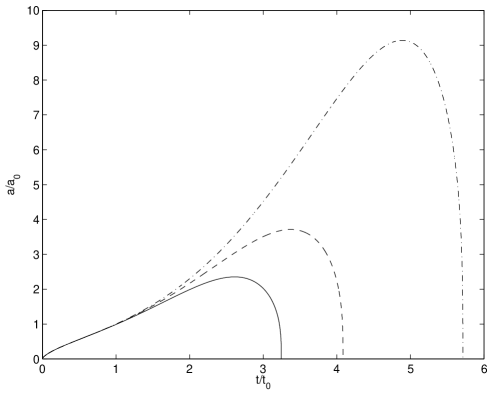
Figure 1: The evolution of the scale factor as a function of physical time for $\omega_{\phi 0}=-0.8,-0.9,-0.95$ (solid line, dashed line and dot-dashed lines respectively). The closer $\omega_{\phi 0}$ is to $-1$ the larger is the total lifetime of the universe.

3 Results and discussion

In Fig. 1 we plot the evolution of the scale factor (in units of $a_{0}$) as a function of physical time (in units of $t_{0}$) for $\omega_{\phi 0}=-0.8,-0.9,-0.95$ (solid line, dashed line and dot-dashed lines respectively). Note that since all the models considered have $\omega_{\phi 0}\sim-1$ the age of the universe at the present time is approximately the same for all the $3$ models considered. We see that all the models have a matter dominated phase with $a\propto t^{2/3}$ followed by an accelerating phase with ${\ddot{a}}>0$ and then by a rapid collapse. It is also obvious from Fig. 1 that the closer $\omega_{\phi 0}$ is to $-1$ the longer is duration of accelerating phase and hence the larger is the total lifetime of the universe.

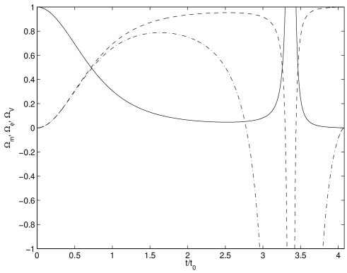
Figure 2: The evolution of $\Omega_{m}$, $\Omega_{\phi}$ and $\Omega_{V}\equiv V(\phi)/H^{2}$ (solid, dashed and dot-dashed lines respectively) as a function of cosmic time for the model with $\omega_{\phi 0}=-0.9$

In Fig. 2 we plot the evolution of $\Omega_{m}$, $\Omega_{\phi}$ and $\Omega_{V}\equiv V(\phi)/H^{2}$ (solid, dashed and dot-dashed lines respectively) as a function of cosmic time for the model with $\omega_{\phi 0}=-0.9$. Again we see that the universe has $\Omega_{m}\sim 1$ at early times and then starts to accelerate near the present time. In the accelerating phase the evolution of $\phi$ is slow and the main contribution to the energy density of the universe comes from $V(\phi)$. During most of this phase $\Omega\sim\Omega_{V}\sim 1$. At some point the energy density of the scalar field $\phi$ becomes small enough and the dynamics of the universe is again dominated by matter and the universe starts decelerating again. Later on $V(\phi)$ turns negative and the universe starts collapsing very rapidly with the energy density being dominated by the kinetic energy density of the scalar field $\phi$. In this phase ${\dot{\phi}}\propto a^{-3}$ and $a\propto(t_{U}-t)^{1/3}$, where $t_{U}$ is the total lifetime of the universe.

In Fig. 3 we plot the fraction, $f$, of the total lifetime of the universe which lies within the interval $[t_{0}-\Delta t_{A},t_{0}+\Delta t_{A}]$ where $t_{0}$ is the age of the Universe at the present time, $\Delta t_{A}\equiv t_{0}-t_{A}$ and $t_{A}$ is age of the universe when it starts to accelerate. We see that $f$ is a increasing function of $\omega_{\phi 0}+1$ and that for $\omega_{\phi 0}$ close to $-1$ there is an almost linear relation between $f$ and $\omega_{\phi 0}+1$. This linear relation is to be expected since for $\omega_{\phi 0}$ very close to $-1$ most of the lifetime of the universe is spent in the accelerating phase. During most of the accelerating phase $V\sim V_{0}$ so that we may estimate the variation of the value of $\phi$ by

$$\Delta\phi\sim\frac{V_{0}}{dV/d\phi}\,.$$ (11)

However, in this phase the scalar field $\phi$ is slowly rolling down the scalar field potential with $3H{\dot{\phi}}\sim-dV/d\phi$. Hence, we have that

$$\Delta\phi\propto-\frac{dV}{d\phi}\Delta\ln a\propto-\frac{dV}{d\phi}\Delta t\,,$$ (12)

where $\Delta t$ is the duration of the accelerating phase. From eqns. (11) and (12) we see that

$$\Delta t\propto\left(\frac{dV}{d\phi}\right)^{-2}\propto\left(\omega_{\phi}+1\right)^{-1}\,,$$ (13)

so that $f\equiv 2(t_{0}-t_{A})/t_{U}\propto\omega_{\phi}+1$ for large enough $t_{U}$ which is confirmed by looking at Fig. 3 (note that for $t_{U}$ sufficiently large $\Delta t\sim t_{U}$). We note that the value of $f$ for which the observed value of $t_{A}$ could be considered a coincidence is of course not well defined. However, from Fig. 3 we see that if we require $f$ to be larger than $0.1$ ($0.01$) then $1+\omega_{\phi 0}\mathrel{\hbox to0.0pt{\lower 4.0pt\hbox{\hskip 1.0pt$\sim$}\hss}\raise 1.0pt\hbox{$>$}}2\times 10^{-2}$ ($1\times 10^{-3}$).

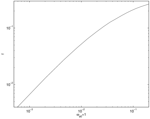
Figure 3: The fraction, $f$, of the total lifetime of the universe which lies within the interval $[t_{0}-t_{A},t_{0}+t_{A}]$ as a function of $\omega_{\phi 0}$. Here $t_{0}$ and $t_{A}$ are respectively the age of the universe at the present time and when it starts to accelerate. Note that $f$ is a decreasing function of $\omega_{\phi 0}$ and that for $\omega_{\phi 0}$ close to $-1$ there is an almost linear relation between $f$ and $\omega_{\phi 0}+1$.

4 Conclusions

In this paper we have investigated the coincidence problem in the context of a generic class of linear dark energy models. If we require our model to satisfy current observational constraints providing at the same time a solution to the coincidence problem then $2\times 10^{-2}(1\times 10^{-3})\mathrel{\hbox to0.0pt{\lower 4.0pt\hbox{\hskip 1.0pt$\sim$}\hss}\raise 1.0pt\hbox{$<$}}1+\omega_{\phi 0}\mathrel{\hbox to0.0pt{\lower 4.0pt\hbox{\hskip 1.0pt$\sim$}\hss}\raise 1.0pt\hbox{$<$}}0.4$. Of course the lower limit depends on how conservative our criterion is. We again emphasize that our results depend mainly on the linearity of the scalar field potential for $-V(\phi_{0})\mathrel{\hbox to0.0pt{\lower 4.0pt\hbox{\hskip 1.0pt$\sim$}\hss}\raise 1.0pt\hbox{$<$}}V(\phi)\mathrel{\hbox to0.0pt{\lower 4.0pt\hbox{\hskip 1.0pt$\sim$}\hss}\raise 1.0pt\hbox{$<$}}V(\phi_{0})$ and are weakly dependent on the specific form of $V(\phi)$ outside this range. It is very interesting that a straightforward solution to the coincidence problem in the simplest generalization of the standard cosmological constant scenario would require a significant departure of $\omega_{\phi 0}$ from $-1$ which may eventually be measured by the next generation of cosmological observations [27].

References

References

- [1] S. Perlmutter et al., Astrophys. J. 517, 565 (1999), astro-ph/9812133.
- [2] A. G. Riess et al., Astrophys. J. 560, 49 (2001), astro-ph/0104455.
- [3] J. Tonry et al., Astrophys. J. 594, 1 (2003), astro-ph/0305008.
- [4] C. L. Bennett et al. Astrophys. J. Suppl. 148, 1 (2003), astro-ph/0302207.
- [5] D. N. Spergel et al. Astrophys. J. Suppl. 148, 175 (2003), astro-ph/0302209.
- [6] S. M. Carroll, Living Rev. Rel. 4, 1 (2001), astro-ph/0004075.
- [7] C. Armendariz-Picon, V. Mukhanov and P. J. Steinhardt, Phys. Rev. D63, 103510 (2001), astro-ph/0006373.
- [8] L. Wang, R. Caldwell, J. Ostriker and P. Steinhardt, Astrophys. J. 530, 17 (2000), astro-ph/9901388.
- [9] M. Bucher and D. N. Spergel, Phys. Rev. D60, 043505 (1999), astro-ph/9812022.
- [10] J. Bagla, H. Jassal and T. Padmanabhan, Phys. Rev. D67, 063504 (2003), astro-ph/0212198.
- [11] P. P. Avelino and C. J. A. P. Martins, Astrophys. J. 565, 661 (2002), astro-ph/0106274.
- [12] M. Malquarti, E. J. Copeland, and A. R. Liddle, Phys. Rev. D68, 023512 (2003), astro-ph/0304277.
- [13] S. Dodelson, M. Kaplinghat and E. Stewart, Phys. Rev. Lett. 85, 5276 (2000), astro-ph/0002360.
- [14] K. Griest, Phys. Rev. D66, 123501 (2002), astro-ph/0202052.
- [15] L. P. Chimento, A. S. Jakubi, D. Pavon, and W. Zimdahl, Phys. Rev. D67, 083513 (2003), astro-ph/0303145.
- [16] L. P. Chimento, A. S. Jakubi, and D. Pavon, Phys. Rev. D67, 087302 (2003), astro-ph/0303160.
- [17] G. Huey and B. Wandelt (2004), astro-ph/0407196.
- [18] R. J. Scherrer, (2004), astro-ph/0410508.
- [19] R.-G. Cai, and A. Wang, (2004), hep-th/0411025.
- [20] R. R. Caldwell, Phys. Lett. B545, 23 (2002), astro-ph/9908168.
- [21] R. R. Caldwell, N. N. Weinberg, and M. Kamionkowski, Phys. Rev. Lett. 91, 071301 (2003), astro-ph/0302506.
- [22] S. Nesseris, and L. Perivolaropoulos, (2003), astro-ph/0410309.
- [23] S. M. Carroll, M. Hoffman, and M. Trodden, Phys. Rev. D68, 023509 (2003), astro-ph/0301273.
- [24] T. Brunier, V. K. Onemli, and R. P. Woodard, (2004), gr-qc/0408080.
- [25] S. Nojiri, and S. D. Odintsov, (2004), hep-th/0408170.
- [26] Y. Wang, J. M. Kratochvil, A. Linde and M. Shmakova (2004), astro-ph/0409264.
- [27] R. Kallosh, J. M. Kratochvil, A. Linde, E. V. Linder and M. Shmakova, JCAP 0310, 015 (2004), astro-ph/0307185.
- [28] P. P. Avelino, C. J. A. P. Martins and J. C. R. E Oliveira, Phys. Rev. D70, 083506 (2004), astro-ph/0402379.
- [29] R. R. Caldwell, and M. Doran, Phys. Rev. D69, 103517 (2004), astro-ph/0305334.